Risk Assessment for Energy Stations Based on Real-Time Equipment Failure Rates and Security Boundaries

Abstract

In the context of China’s 2020 dual carbon goals of peak CO₂ emissions by 2030 and carbon neutrality by 2060, the security of multi-energy systems is increasingly challenged as clean energy continues to be supplied to the system. This paper proposes a risk assessment and enhancement strategy for distributed energy stations (DESs) based on a security boundary. First, based on the coupling relationship between different energy sources and combining the mutual support relationships between different pieces of equipment, a security boundary for DESs was constructed. Second, based on the characteristics of different sources of equipment failure, the real-time failure probabilities of equipment and pipelines were calculated in order to obtain the security risks of DES operation states based on the security boundary. Finally, for equipment and pipelines at high risk, an economic security enhancement strategy is proposed, and the Pareto solution set is solved using a multi-objective algorithm. The analysis shows that the proposed method can effectively quantify the security risks of energy systems in real time, and the proposed enhancement strategy takes into account both economics and system security.

1. Introduction

With the increasing integration of large quantities of new energy and the growing diversification of loads, the power grids and equipment associated with distributed energy stations (DESs) are gradually becoming more complex and diverse [1,2]. At the same time, the coupling between heterogeneous energy sources is deepening, and any failure in the energy network on one side of a DES may be transmitted to other stations in the network through coupling nodes. For example, in August 2019, a gas station failure in the UK led to low-frequency load shedding in the power grid, causing widespread power supply disruptions. Natural disasters and random unexpected failures pose serious challenges to the stable operation of DESs [3,4], significantly affecting users’ experiences of using energy and society’s energy security. Therefore, it is of great importance and technical value to conduct in-depth research into risk assessment and improvement methods for DESs in the context of random disasters and disturbances.

The security risk assessment of individual energy networks has always been a hot topic of research, and there is already a substantial body of research on the security risks of power systems. The stochastic nature of new energy sources and loads in power systems increases the probability of accidents to some extent [5]. In [6], a risk assessment method for wind power transmission systems is presented, taking into account the correlation between wind resources and loads. In [7], the uncertainty of new energy generation and loads in microgrids is considered, and the probability of power shortages is quantitatively evaluated. Probabilistic power flow, which considers interval characteristics, is widely used to characterize the uncertainties associated with new energy sources and loads [8]. Using the probabilistic power flow method, it is possible to monitor power transformer overloads [9], line overloads [9], voltage violations [10], and other operational risks in the power system. Currently, there is limited research on the security risks of individual natural gas and heat networks. In [11], gas pipeline risk is assessed based on the probability of the occurrence of adverse events and system vulnerability coefficients. In [12], a risk assessment of heat exchangers and the entire heat transfer network is performed, considering the overall system risk. The above security risk studies are only applicable to single energy networks and are not suitable for the broader context of multi-energy and coupled energy systems.

Recently, there have been some studies on the security risk assessment of multi-energy coupled systems; however, they have focused mainly on long-term security risks. In [13], the dynamic characteristics of natural gas and thermal systems are used to propose a method for calculating optimal energy flow for multi-energy systems during accidents, aiming to reduce energy losses during such incidents. The correlation and volatility of energy raw material prices also affect the operational risks of multi-energy systems. In [14], a risk assessment model for energy price uncertainty is developed, and the impact of extreme price uncertainty is quantified using conditional value-at-risk. In [15], a novel risk index that considers the benefits of each operator is introduced to comprehensively describe the security risks of multi-energy coupled systems and the interests of each operator. The semi-invariant method [16] is widely used in risk assessment. In [17], risk parameters such as pressure, frequency, and power are selected in order to calculate the probability distribution of state variables using the semi-invariant method, thereby obtaining a quantitative risk value for the system. Some researchers use interval theory to analyze the security of regional energy systems utilizing renewable energy [18]. In [19], robust security regions are constructed using convex hulls applicable to multi-energy coupled systems to evaluate the operational security of the system. In [20], a real-time scheduling model considering conditional value-at-risk is developed to analyze cost-at-risk for overestimated and underestimated cost scenarios. However, current studies focus mainly on the operational risks arising from random fluctuations of new energy sources and loads, and there is limited research on the risk analysis of distributed energy resources under real-time failure probabilities.

In order to address these problems, this paper carried out a study of the risk assessment and response strategies of DESs, considering system security boundaries and equipment failure rates. Firstly, we analyzed the mutual backup relationship of different pieces of equipment and pipelines and constructed a security boundary model by incorporating the multi-energy flow balance equation; secondly, we propose a method for quantifying the real-time failure probability of equipment and pipelines by integrating the effects of equipment health status, weather conditions, and other risk sources. Finally, we propose an optimal response strategy for energy storage, considering both security and economics for high-risk equipment or pipelines. The analysis showed that the proposed security risk assessment method can effectively quantify the real-time operational risks of energy stations, and the proposed strategy can optimize the energy storage allocation for high-risk nodes, which has particular significance for practical engineering applications.

2. DESs and Security Risk

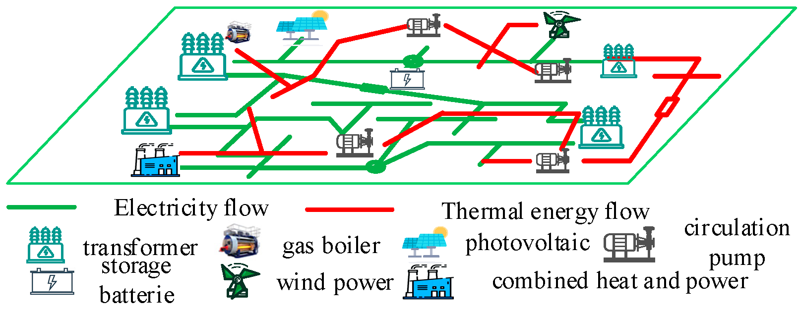
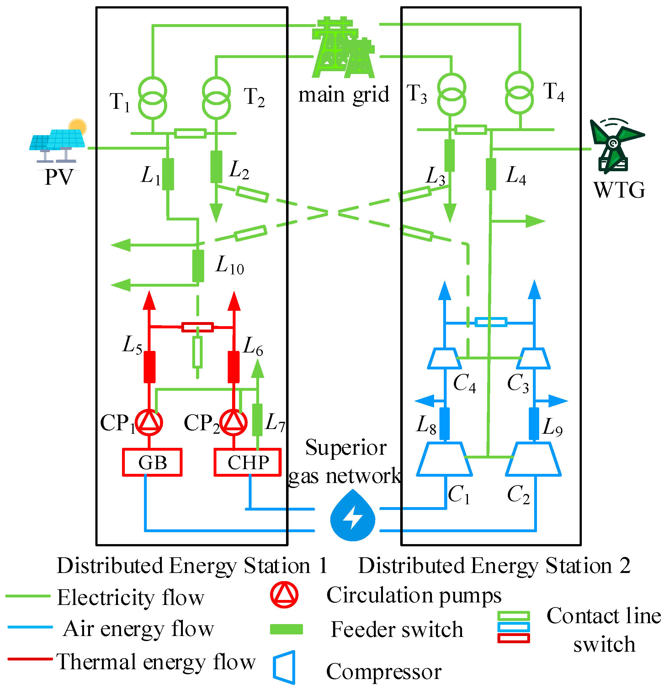
2.1. DESs

DESs are located on the user side of energy networks and have inherent locational advantages, allowing for the localized consumption of renewable energy [21]. They integrate traditional energy networks with diversified energy demands and supplies, enabling the coupling and coordination of various energy flows in order to achieve efficient utilization of energy and the integration of renewable energy. An interconnected regional DES is illustrated in Figure 1. The DES is built upon the existing power grid and natural gas network and expands the regional heating network based on user demand. To enhance the security and reliability of energy supply, the two regional distribution networks are interconnected through tie lines for power transmission, while the regional gas and heating networks are interconnected through multiple sources to ensure mutual energy supply between regions.

2.2. Security Risk Assessment

The security of a DES refers to its ability to provide uninterrupted and reliable energy to users even in the event of random failures, such as sudden short circuits or unplanned component failures. This is one of the important considerations for ensuring the security and stable operation of the energy station. Compared to the main grid, DESs have a lesser ability to withstand failures. Therefore, a real-time understanding of the security risks of energy stations becomes particularly critical. In the engineering field [22], the classic definition of risk R is given by

$$R=\{\langle S_i,P_i,x_i\rangle \},$$

(1)

where S_i represents the scenario where the failure occurred, P_i is the probability of the scene occurring, and x_i represents the degree of harm in this scenario. The failure scenario of the energy station can be determined through the predicted accident set; the probability of scenario occurrence is determined by the probability of equipment failure; and the degree of harm in the scenario is determined by the relationship between the real-time operating status of the energy station and the security boundary. The real-time operation status of the energy station alone cannot directly determine the operation status of the energy station after equipment failure. Therefore, the safety boundary is introduced to determine the operation status of the energy station after equipment failure more quickly and intuitively. The safety boundary refers to the maximum energy supply boundary of the energy system in the event of a N-1 failure of equipment or pipeline [23]. Its model can be expressed as

$$M=\left\{L|f(L)=0,g(L)\le 0\right\}$$

(2)

where L is the energy station operating state observation; $f(L)=0$ denotes the energy station N-1 faulty operation equation constraint; and $g(L)\le 0$ denotes the energy station N-1 inequality constraint. Therefore, this study analyzed the real-time security risk of energy stations from the perspective of security boundaries and equipment failure probability.

3. Security Boundary Analysis Based on Mutual Backup Relationships

By constructing a set of foreseen accidents to determine the failure scenarios, it is possible to explore the mutual backup support relationships between the different pieces of equipment or pipelines under the failure scenarios and calculate the safety boundaries for each piece of equipment in order to quantify the degree of harm from the different failure scenarios.

3.1. Hypothetical Accident Set

The output power of the transmission outlet pipeline is representative of the overall operation of the energy station. It is subject to the capacity limitations of the connected equipment and pipelines and possesses the capability of flow optimization control [24]. Therefore, the transmission pipelines are selected as the object for operational status monitoring, with the front end connected to the key equipment and the back end facing the customer side. The energy station operating state vector L = [L₁, L₂, …, L_m] is defined to represent the operating state of m key pipelines.

The selected types of random accidents in this study included two main categories: (1) key equipment failures, such as those of transformers, circulating pumps, and combined heat and power (CHP) units; and (2) key pipeline failures, such as those of power buses. By constructing a hypothetical accident set, the weak links in the operational state of the energy station can be identified, thus optimizing its operational state. The hypothetical accident set considers both causal factors, such as capacity configuration between different pieces of equipment, and backup relationships between different components. The symbols in the text are explained in Appendix A.

3.2. Constraint on Multi-Energy Flow Balance

When random failures occur, maintaining the stable operation of an energy station requires fulfilling the energy balance relationships of multiple systems, including the power, thermal, and natural gas systems.

3.2.1. Power System Energy Balance Equation

In the steady-state model of the power system [25], the effects of three-phase imbalance are neglected, and the power flow calculation model is given by

$$P_i=U_i{\displaystyle \sum _{j\in i}{U}_j(G_{ij}\cos {\theta }_{ij}+B_{ij}\sin }{\theta }_{ij}),$$

(3)

$$Q_i=U_i{\displaystyle \sum _{j\in i}{U}_j(G_{ij}\sin {\theta }_{ij}-B_{ij}\cos {\theta }_{ij})},$$

(4)

where P_i and Q_i represent the active power and reactive power of the ith node, respectively, G_ij and B_ij represent the conductance and susceptance between nodes i and j, respectively, and θ_ij represents the phase angle difference between nodes i and j.

CHP units enable combined heat and power production and are important for electrical and thermal coupling. The model is described as

$$C_{\mathrm{CHP}}=\frac{P_{\mathrm{CHP},\mathrm{h}}}{P_{\mathrm{CHP},\mathrm{e}}},$$

(5)

where C_CHP represents the thermal-to-electric ratio of the CHP unit, which typically ranges from 1.5 to 10, and P_CHP,h and P_CHP,e represent the thermal and electric power outputs.

3.2.2. Gas System Energy Balance Equation

The model for calculating the natural gas flow [26] containing the compressor is given by

$$f_{ij}=\mathrm{sgn}{k}_{ij}\sqrt{\mathrm{sgn}(p_i^2-p_j^2)},$$

(6)

where f_ij represents the flow from node i to node j, sgn is the sign function, which takes the value 1 when the pressure at node i is greater than that at node j, and −1 otherwise, and k_ij is the pipe coefficient.

The natural gas transmission process involves pressure loss, which requires the use of compressors for pressurization. The electric compressor model can be described as

$$P=\frac{0.7457Q_{a}C}{{10}^3}(K^{\frac{a-1}{a}}-1),$$

(7)

where K represents the compression ratio, C is the coefficient related to temperature and efficiency, a is a variable coefficient, and Q_a is the compressor flow rate.

3.2.3. Thermal System Energy Balance Equation

The thermal system transfers energy through a medium without, in theory, consuming the medium itself. By applying the principle that the sum of the heads is zero, we can derive the flow model [27] for the thermal system as follows:

$$B{h}_f=B{K}_{g}m\left|m\right|=0,$$

(8)

where B represents the correlation matrix of the network, m is the branch flow vector, and K_g represents the pipe coefficient, which is given by:

$$K_g=\frac{8Lf}{D^5{\rho }^2\pi g},$$

(9)

where L represents the pipe length, f represents the pipe friction, D represents the pipe diameter, ρ represents the density of the medium, and g is taken as 9.8. The relationship between node power and flow can be expressed as

$$P=C_{\mathrm{w}}m(T_{\mathrm{o}}-T_{\mathrm{i}}),$$

(10)

where C_w represents the specific heat capacity of the medium, m represents the flow rate in the pipe, and T_o and T_i represent the outlet and return water temperatures, respectively. T_o can be expressed as

$$T_{\mathrm{o}}=T_{\mathrm{a}}+(T_{\mathrm{i}}-T_{\mathrm{a}})\exp (-\frac{\lambda L}{{\mathrm{C}}_{\mathrm{w}}m}),$$

(11)

where T_a represents the ambient temperature and λ represents the heat transfer coefficient.

The thermal system requires a circulating pump to maintain system operation, and its required power is given by

$$P_s=\frac{m(p_{\mathrm{out}}-p_{\mathrm{in}})}{{10}^6\eta \rho },$$

(12)

where η represents the efficiency of the circulation pump, p_out and p_in are the outlet and inlet pressures of the medium, respectively, and ρ is the density of the medium.

The energy sources in the thermal system include gas boilers and CHP units. Since the CHP unit has already been modeled in the power system, this section focuses only on the gas boiler. The equation for modeling the gas boiler is given by

$$P_{\mathrm{GB}}=\beta Hm,$$

(13)

where P_GB represents the power output of the gas boiler, β is the boiler efficiency, H is the average heating value of natural gas, and m is the natural gas consumption flow rate of the gas boiler.

By decoupling the multi-energy coupled equipment and separating the different energy subsystems, the power flow calculation is performed using the power flow method. Current power flow calculation methods are mature and will not be described here [16].

3.3. Boundary Analysis Based on Mutual Standby Relationships

In energy stations, standby relationships are common. When a failure occurs, two pieces of equipment (pipelines) or multiple pieces of equipment (pipelines) having a standby relationship with each other can support the load and replace the failed equipment (pipelines). At the same time, in order to improve the security of the energy station, a backup relationship can be formed between two pieces of equipment (pipelines) or multiple pieces of equipment (pipelines) through a contact pipeline. In this paper, the key pipeline output power is selected as the research object for analyzing two types of standby situations for equipment and pipelines.

The first category of cases is the mutual backup relationship for critical equipment. The key equipment is connected to the transmission outlet pipeline, and its boundary model is given by

$${\displaystyle \sum C_i}+{\displaystyle \sum L_i^{\mathrm{sub}}}\le {\displaystyle \sum L_i}\le {\displaystyle \sum S_m}+P+W,$$

(14)

where ${\displaystyle \sum L_i}$ is the sum of the power outputs of the transmission outlet pipeline connected to the mutual standby related equipment, ${\displaystyle \sum C_i}$ is the sum of the power required for the normal operation of the coupled equipment (including circulating pumps, compressors, etc.), ${\displaystyle \sum L_i^{\mathrm{sub}}}$ is the sum of the power outputs of the lower pipeline of the transmission outlet pipeline, P and W are the power outputs of photovoltaic power generation and wind power generation, respectively, connected to the transmission outlet pipeline, ${\displaystyle \sum S_m}$ is the sum of the standby outputs of other equipment under conditions of failure of the equipment, and S_m represents the corresponding pipeline constraints and equipment capacity constraints, the formula for which is given by

$$S_m=\min [C_m^{\mathrm{EQ}}-L_m,C_m^{\mathrm{TL}}-L_m],$$

(15)

where $C_m^{\mathrm{EQ}}$, $C_m^{\mathrm{TL}}$ represent the capacity of the mth backup equipment and the backup equipment connected to the pipeline capacity, respectively, and L_m represents the mth standby equipment connected to the line with the load power.

The second type of situation is the mutual backup relationship between key pipelines. Due to the complexity of the pipeline network frame, there are generally multiple standby ways. The pipeline L_a boundary model is given by

$${\displaystyle \sum C_i}+{\displaystyle \sum L_i^{\mathrm{sub}}}\le L_{\mathrm{a}}\le {\displaystyle \sum S_i}+\max (S_i^{\mathrm{com}})+P+W,$$

(16)

where S_i^com is the output power of the ith mutually incompatible backup mode. Among these backup relationships, the maximum output backup mode needs to be taken. ΣS_i is the sum of the outputs of the backup modes without competing relationships. S_i^com and S_i both contain pipeline capacity and equipment capacity constraints, and the equations are given by

$$\{\begin{array}{l}{S}_i=\min [C_i^{\mathrm{EQ}}-L_i,C_i^{\mathrm{TL}}-L_i]\\ S_i^{\mathrm{com}}=\min [C_i^{\mathrm{EQ},\mathrm{com}}-L_i^{\mathrm{com}},C_m^{\mathrm{TL},\mathrm{com}}-L_i^{\mathrm{com}}]\end{array},$$

(17)

where $C_i^{\mathrm{EQ}}$, $C_i^{\mathrm{TL}}$ represent the ith mutually incompatible backup mode equipment capacity and the pipeline capacity, respectively, $C_i^{\mathrm{EQ},\mathrm{com}}$, $C_i^{\mathrm{TL},\mathrm{com}}$ represent the noncompetitive relationship backup mode equipment capacity and the pipeline capacity, respectively; and L_i, L_i^com represent the ith mutually incompatible and noncompetitive relationship backup mode pipeline, respectively, with the load power. Taking Figure 2 as an example, the following analysis is for the relevant backup relationship and boundary situation of the energy station.

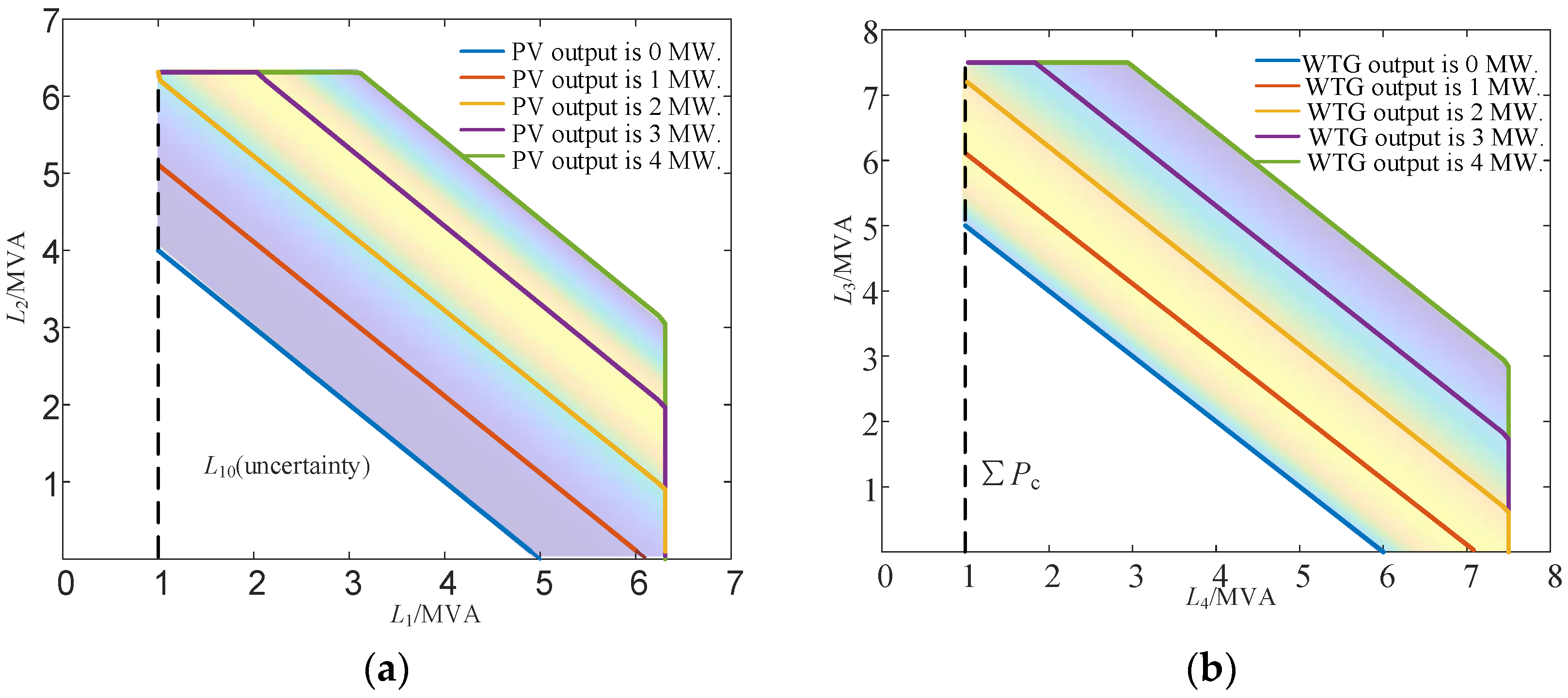
3.3.1. Probability of Renewable Energy Contribution

The security boundary of an energy station varies with the output of renewable energy. Probabilistic modeling of renewable energy output can explore the law of energy station security boundary change with renewable energy output.

The two-parameter-based Weibull model is widely used for stochastic probabilistic modeling of wind turbines [28]. The wind power probability distribution P_wout is given by

$$f(V_{\mathrm{h}})=(\frac{k_{\mathrm{w}}}{c_{\mathrm{w}}}){(\frac{V_{\mathrm{h}}}{c_{\mathrm{w}}})}^{(k_{\mathrm{w}}-1)}\exp [-{(\frac{V_{\mathrm{h}}}{c_{\mathrm{w}}})}^{k_{\mathrm{w}}}];$$

(18)

$$P_{\mathrm{wout}}=\{\begin{array}{l}0,0\le V_{\mathrm{h}}\le V_{\mathrm{in}},V_{\mathrm{out}}\le V_{\mathrm{h}}\\ {\mathrm{P}}_{\mathrm{wmax}}\frac{V_{\mathrm{h}}-{\mathrm{V}}_{\mathrm{in}}}{{\mathrm{V}}_{\mathrm{r}}{-\mathrm{V}}_{\mathrm{in}}},V_{\mathrm{in}}\le V_{\mathrm{h}}\le V_{\mathrm{r}}\\ {\mathrm{P}}_{\mathrm{wmax}},V_{\mathrm{r}}\le V_{\mathrm{h}}\le V_{\mathrm{out}}\end{array},$$

(19)

where k_w is the shape factor, c_w is the scale factor, V_r, V_h, V_out, and V_in are the rated wind speed, actual wind speed, cut-out wind speed, and cut-in wind speed, respectively, and P_wmax is the maximum output power of the fan.

For the probability distribution of a photovoltaic (PV) power output, a model based on the beta probability distribution can give better results [29]. The power output model of the PV generator set can be expressed as

$$f(S_{\mathrm{h}})=\frac{\mathsf{\Gamma }({\alpha }_{\mathrm{p}}+{\beta }_{\mathrm{p}})}{\mathsf{\Gamma }({\alpha }_{\mathrm{p}})\mathsf{\Gamma }({\beta }_{\mathrm{p}})}{(\frac{S_{\mathrm{h}}}{S_{\mathrm{r}}})}^{{\alpha }_{\mathrm{p}}-1}{(1-\frac{S_{\mathrm{h}}}{S_{\mathrm{r}}})}^{{\beta }_{\mathrm{p}}-1},$$

(20)

$$P_{\mathrm{pv},\mathrm{out}}=\{\begin{array}{l}{P}_{\mathrm{pv},\max }\frac{S_{\mathrm{h}}}{S_{\mathrm{r}}},S_{\mathrm{h}}\le S_{\mathrm{r}}\\ P_{\mathrm{pv},\max },S_{\mathrm{h}}>S_{\mathrm{r}}\end{array},$$

(21)

where a_p, β_p are shape and scale factors, respectively, S_h, S_r are the actual and rated light intensities, respectively, and P_pv,max is the maximum PV power.

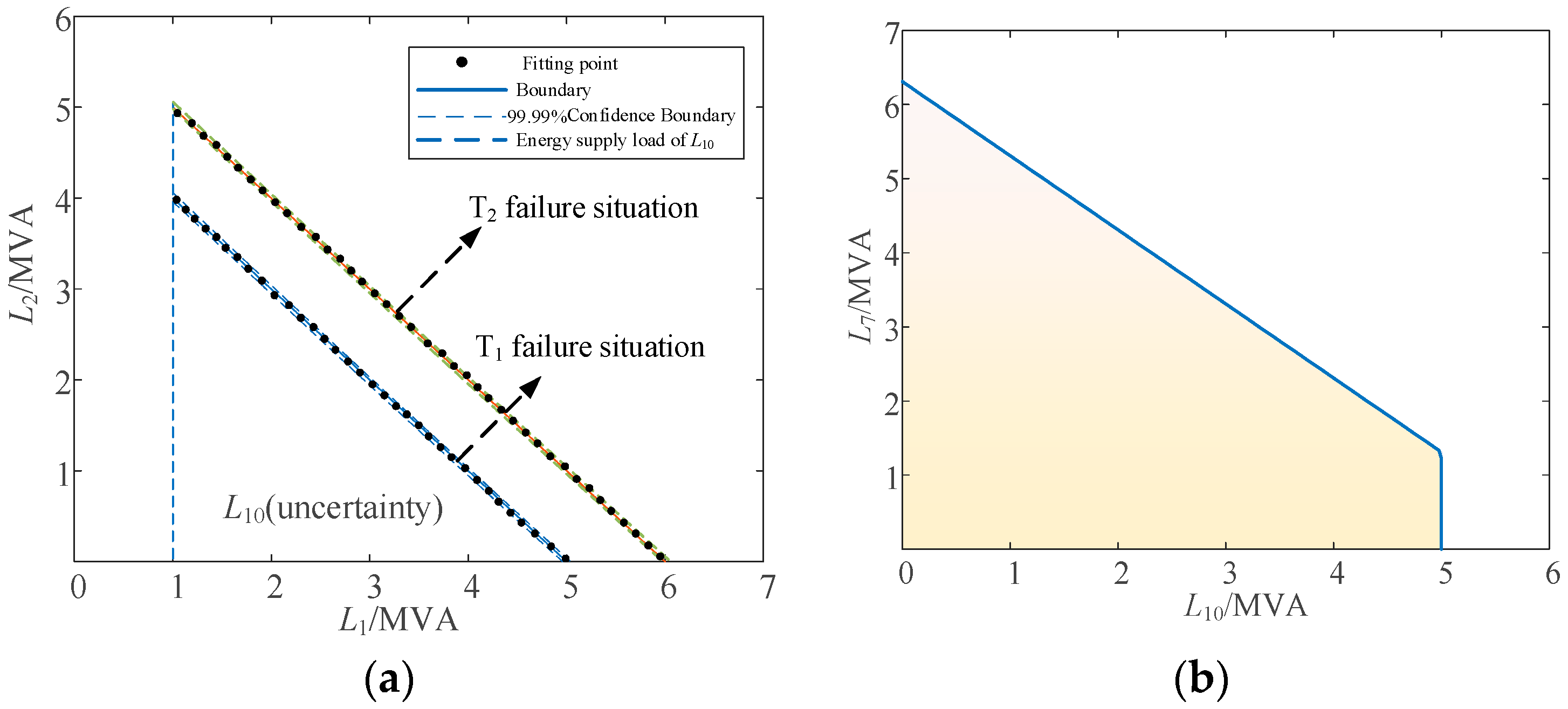
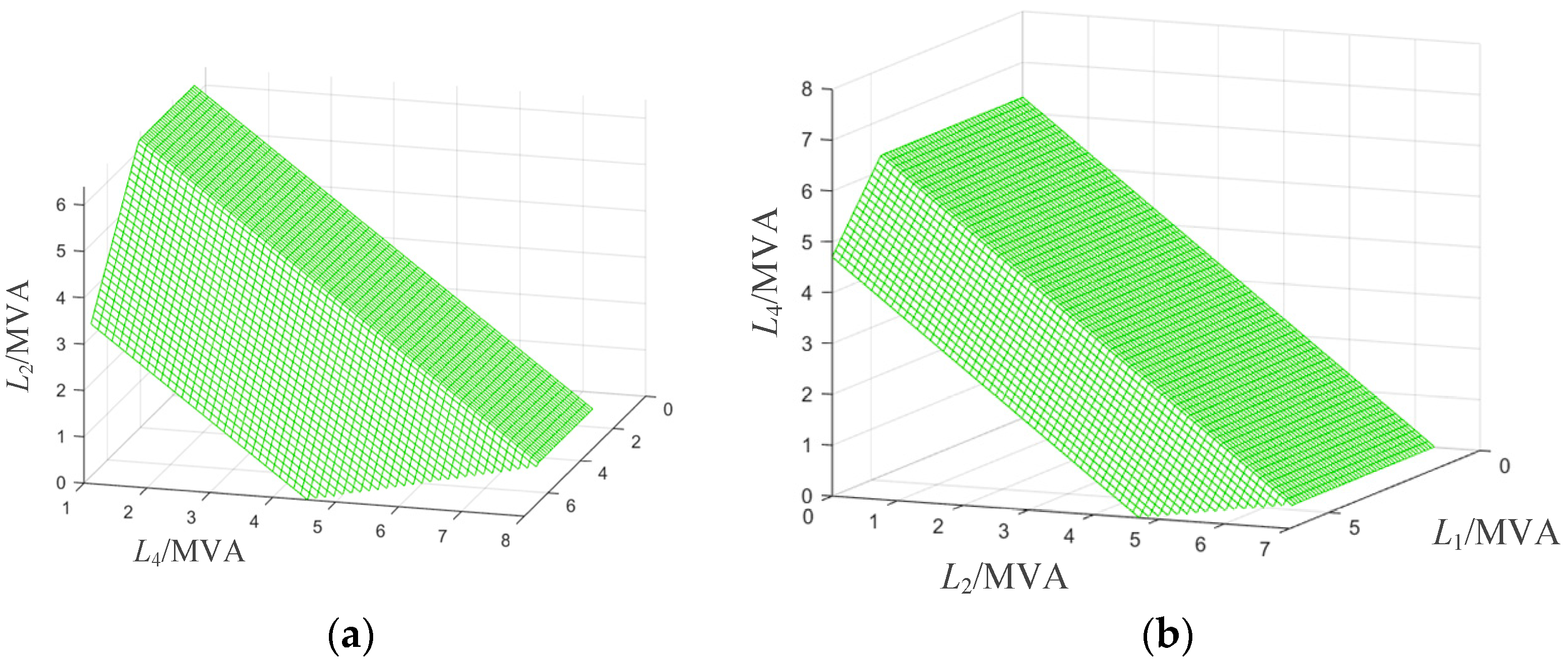
3.3.2. Power System Boundary Analysis

The power critical equipment includes CHP units, transformers {T₁, T₂, T₃, T₄}, and critical pipelines L = {L|L₁, L₂, L₃, L₄, L₇, L₁₀}. Since there are obvious differences between equipment failures and pipeline failures, the two are analyzed separately below.

When a failure occurs in transformer T₁ or T₂, the load carried by the failed transformer can be transferred to another transformer by means of a contact switch between them. Although PV power generation plays a certain role in supplementing the energy of the failed load, it also leads to the problem of probabilistic T₁ and T₂ boundaries, where the {T1, T2} boundary model is given by

$$\{\begin{array}{l}{L}_{10}<L_1\\ L_1+L_2<\min (C_{\mathrm{T}1},C_{\mathrm{T}2})+P_{\mathrm{pv},\mathrm{out}}\end{array}.$$

(22)

Similarly, wind power generation also probabilizes the T₃ and T₄ boundaries. The {T₃, T₄} boundary model can be expressed as

$${\displaystyle \sum P_{Ci}}<L_3+L_4<\min (C_{\mathrm{T}3},C_{\mathrm{T}4})+P_{\mathrm{wout}}.$$

(23)

When the CHP unit fails, its load will be supplied by the L₁₀ feeder via the contact line, and the CHP power boundary model is given by

$$(P_{\mathrm{CP}1}+P_{\mathrm{CP}2})<L_{10}<(C_{L10}-L_7).$$

(24)

When the pipeline fails, energy can be supplied to the failed load through other backup pipelines or contact pipelines. When L₂ fails, DES 2 supplies energy to the failed load at another station, and the L₂ boundary model is given by

$$0<L_2<\min [(C_{\mathrm{T}3}+C_{\mathrm{T}4}+P_{\mathrm{wout}}-L_3-L_4),(C_{L4}-L_4\left)\right].$$

(25)

When L₄ fails, DES 1 supplies energy to L₄, and the L₄ boundary model is given by

$$\{\begin{array}{l}{L}_2+L_4>(P_{\mathrm{C}1}+P_{\mathrm{C}2}+P_{\mathrm{C}3}+P_{\mathrm{C}4}),\\ L_4<\min [(C_{\mathrm{T}1}+C_{\mathrm{T}2}+P_{\mathrm{pv},\mathrm{out}}-L_1-L_2),\\ (C_{L2}-L_2\left)\right].\end{array}$$

(26)

For the associated pipeline {L₇, L₁₀}, when L₁₀ fails, energy is supplied by the CHP unit to the failed line L₁₀. The boundary model for L₁₀ is given by

$$0<L_{10}<\min (C^{\mathrm{e}}{}_{\mathrm{CHP}}-L_7,C_{L7}-L_7,L_6/C_{\mathrm{CHP},\min }),$$

(27)

where C^e_CHP is the maximum electrical capacity of the CHP unit. When L₇ fails, energy is supplied from L₁₀ to the failed line L₇ via the contact pipelines. The boundary model for L₇ is given by

$$\{\begin{array}{l}{L}_7>P_{\mathrm{CP}1}+P_{\mathrm{CP}2},\\ L_7<\min \{\min [(C_{\mathrm{T}1}+C_{\mathrm{T}2}+P_{\mathrm{pv},\mathrm{out}}-L_1-L_2),\\ (C_{L1}-L_1)]+\min [(C_{\mathrm{T}3}+C_{\mathrm{T}4}+P_{\mathrm{wout}}-L_3-L_4),\\ (C_{L3}-L_3)],(C_{L10}-L_{10})\text{}},\end{array}$$

(28)

For the associated pipeline {L₃, L₁₀, L₁}, when L₃ fails, the transformer set and CHP unit of DES 1 supply energy to L₃ through the contact pipeline, and the L₃ boundary model is given by

$$\{\begin{array}{l}{L}_3>0,\\ L_3<\min [(C_{\mathrm{T}1}+C_{\mathrm{T}2}+P_{\mathrm{pv},\mathrm{out}}-L_1-L_2),\\ (C_{L1}-L_1)]+\min [(C^{\mathrm{e}}{}_{\mathrm{CHP}}-L_7),L_6/C_{\mathrm{CHP},\min },\\ (C_{L7}-L_7),(C_{L10}-L_{10})].\end{array}$$

(29)

When L₁ fails, DES 2 and the CHP unit supply energy to L₁ through the contact line, and then the L₁ boundary model is given by

$$\{\begin{array}{l}{L}_1>0,\\ L_1<\min [(C_{\mathrm{T}3}+C_{\mathrm{T}4}+P_{\mathrm{wout}}-L_3-L_4),\\ (C_{L3}-L_3\left)\right]+\min \left[\right(C^e{}_{\mathrm{CHP}}-L_7),(C_{L7}-L_7),\\ L_6/C_{\mathrm{CHP},\min },(C_{L10}-L_{10}\left)\right].\end{array}$$

(30)

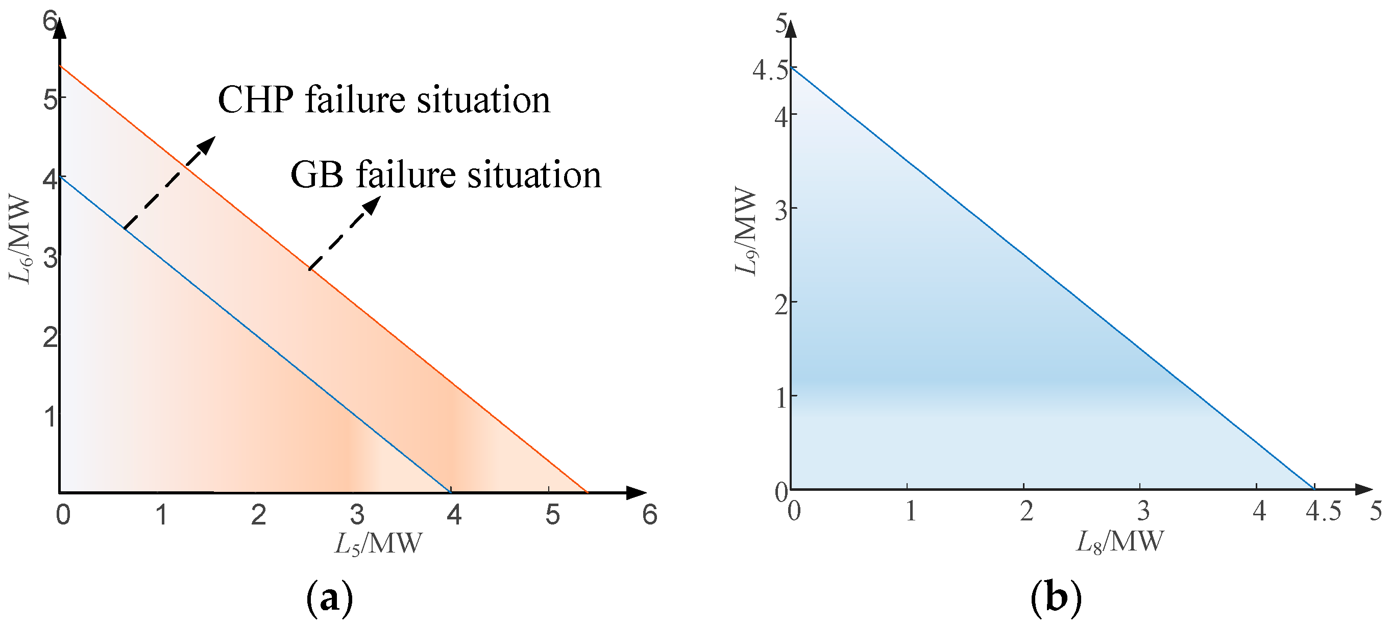
3.3.3. Thermal System Boundary Analysis

The key pieces of equipment in the thermal system are the circulation pumps {CP₁, CP₂}, the gas boiler (GB), the CHP units, and the key pipelines {L₅, L₆}. When the GB, CP₁, or pipeline L₅ fails, the load it carries will be provided by the CHP unit, and then the L₅ GB boundary model is given by

$$0<L_5<\min [(C^{\mathrm{h}}{}_{\mathrm{CHP}}-L_6),(C_{{\mathrm{CP}}_2}-L_6),(C_{L6}-L_6),(C_{\mathrm{CHP},\max }{L}_7-L_6)],$$

(31)

where C^h_CHP is the heat capacity of the CHP unit. When the CHP unit, CP₂, or L₆ fails, the load carried by the failed equipment or pipeline will be provided by the GB and CP₁, and then the L₆ CHP thermal boundary model is given by

$$0<L_6<\min [(C_{\mathrm{GB}}-L_5),(C_{\mathrm{CP}1}-L_5),(C_{L5}-L_5)],$$

(32)

where C_GB is the capacity of the GB.

3.3.4. Natural Gas System Boundary Analysis

The key pieces of equipment in the natural gas system are the compressors {C₁, C₂, C₃, C₄} and the key pipelines {L₈, L₉}. When C₁ or L₈ fails, the load carried by L₈ will be provided by C₂ via L₉ and the contact line, and then the C₁, L₈ boundary model is given by

$$0<L_8<\min [(C_{\mathrm{C}2}-L_9),(C_{L9}-L_9)].$$

(33)

When C₂ or L₉ fails, the load carried by L₉ will be supplied by C₁ via L₈ and the contact line, and the boundary model for C₂ and L₉ is given by

$$0<L_9<\min [(C_{\mathrm{C}1}-L_8),(C_{L8}-L_8)].$$

(34)

3.3.5. Boundary Solving

According to the multi-energy flow balance constraint and the boundary constraint, the maximum output model of the energy station can be expressed as

$$\begin{array}{l}\max {\displaystyle \sum L_i}\\ s.t.\{\begin{array}{l}h(\mathit{L})=0\\ \overline{\mathit{g}}\le g(\mathit{L})\le \underset{\_}{\mathit{g}}\end{array}\end{array}.$$

(35)

where: $h(\mathit{L})=0$ contains the set of Equations (3)–(13); $\overline{\mathit{g}}\le g(\mathit{L})\le \underset{\_}{\mathit{g}}$ contains the set of Equation (22) through Equation (34). The large-scale nonlinear programming problem described by Equation (35) can be better solved using the interior point method. Transforming the problem into the general form of the interior point method, the equations can be solved using Lagrangian functions [22], which are not described here. By fixing some of the load-free variables, a set of boundary point solutions can be found, and the energy station boundary can be obtained by fitting the set of boundary point solutions.

4. Methodology for Assessment of DES Security Risks

4.1. Risk Source-Based Failure Analysis

There are three types of risk sources that lead to the failure of energy station equipment or pipelines: (1) equipment health status: equipment aging, defects, age, etc.; (2) external weather conditions: severe weather, etc.; and (3) other factors: electromagnetic environment, thermal environment, etc. According to the relevant literature and historical data [30], equipment health status and weather conditions are the main factors causing equipment failure. The effects of other risk sources vary from scenario to scenario and need to be evaluated by building corresponding models.

4.1.1. Failure Analysis Based on Equipment Health Status

Equipment failure frequency and equipment health status are closely related. China’s State Grid Corporation issued the document Q/GDW 645-2011 Distribution Network Equipment Condition Evaluation Guidelines in 2011, which provides a theoretical reference for the health status of distribution network equipment. Heat network equipment and gas network equipment can be evaluated in terms of equipment condition based on information obtained from online inspection, operational inspection, degree of equipment aging, equipment service life, and operational status. Based on an idea reported in the literature [31], the relationship between equipment failure frequency f_i,eq and equipment health state S_i is given by

$$f_{i,\mathrm{eq}}=a_i·e^{b_i{S}_i}+c_i,$$

(36)

where i is the number of the piece of equipment, a_i is a proportionality factor, b_i is a curvature factor, and c_i is a constant. The above three coefficients can be derived from the determination of the maximum failure rate f_max, minimum failure rate f_min, and average failure rate f_av of the equipment, and the equations relating them are given by

$$\{\begin{array}{ll}{f}_{\max }=a_i\times e^{b_i{S}_i}+c_i,\hfill & S_i=S_{\min }\hfill \\ f_{\mathrm{av}}=a_i\times e^{b_i{S}_i}+c_i,\hfill & S_i=S_{\mathrm{av}}\hfill \\ f_{\min }=a_i\times e^{b_i{S}_i}+c_i,\hfill & S_i=S_{\max }\hfill \end{array},$$

(37)

where S_min, S_av, and S_max denote the worst, average, and best state ratings of the equipment, respectively.

4.1.2. Failure Analysis Based on Weather Factors

Outdoor equipment can be affected by severe weather, which can significantly increase the frequency of equipment failures [32]. Therefore, weather conditions must be taken into account when performing failure analysis on outdoor equipment and pipelines. Commonly used weather models are two-state and multi-state models. A two-state model is used in this paper. If the severity of the weather needs to be accurately described, the multi-state model can be used, where the weather state quantity w is used to describe the severity of the weather. The failure frequency model based on weather factors f_j,w is given by

$$f_{j,w}=\{\begin{array}{cc}{f}_{j,\mathrm{av}}\frac{N_j+U_j}{N_j}\left(1-K_j\right),& w=0\\ f_{j,\mathrm{av}}\frac{N_j+U_j}{U_j}{K}_j,& w=1\end{array},$$

(38)

where f_j,av is the average failure frequency of the jth piece of equipment, N_j, U_j are the durations of normal and bad weather conditions during the statistical measurement period of the equipment, K_j is the proportion of equipment failure during bad weather: In normal weather, w is taken as 0; in bad weather, w is taken as 1.

4.1.3. Failure Analysis of Other Risk Sources

Other factors, such as the electromagnetic environment and the thermal environment, can also affect the failure frequency of equipment. With the help of weather factor-based failure analysis, the failure model f_j,e for other risk sources is given by

$$f_{j,e}=\{\begin{array}{ll}\frac{n_{j,i}}{N_{j,i}}{K}_{j,i},& e=i\\ ⋮,& ⋮\\ \frac{n_{j,m}}{N_{j,m}}{K}_{j,m},& e=m\end{array},$$

(39)

where i is the ith state under this factor, using a multi-state model with a total of m states, n_j,i is the number of failures of the jth piece of equipment, N_j,i is the time duration of the ith state, and the K_j table is the proportion of failed equipment during bad weather.

4.1.4. Equipment Failure Probability Model

Equipment failure is a random, discrete event whose occurrence is affected by the state of equipment health, weather conditions, and other sources of risk. Equipment failures occur randomly, with a fixed average frequency over time ∆t, and, therefore, the failure probability distribution can be considered a first-order Poisson distribution with respect to time [30]. The probabilities of failure based on equipment state F_eq, weather factors F_w, and other risk sources F_e are given by

$$\{\begin{array}{c}{F}_{\mathrm{eq}}=1-e^{-f_{\mathrm{eq}}\Delta t}\\ F_{\mathrm{w}}=1-e^{-f_{\mathrm{w}}\Delta t}\\ F_{\mathrm{e}}=1-e^{-f_{\mathrm{e}}\Delta t}\end{array},$$

(40)

where ∆t is the measurement period, f_eq is the frequency of failure based on equipment status, f_w is the frequency of failure based on weather conditions, and f_e is the frequency of failure from other risk sources. Although failure events are affected by multiple independent factors, they can occur only once at a certain time. Then, the probability of failure of each factor can be integrated in order to establish the probability model F of equipment failure within the time period ∆t:

$$F=\{\begin{array}{cc}\hfill F_{\mathrm{eq}},\hfill & w=0,e=0\hfill \\ \hfill F_{\mathrm{eq}}+F_e-F_{\mathrm{eq}}·F_e,\hfill & w=0,e=1\hfill \\ \hfill F_{\mathrm{eq}}+F_w-F_w·F_{\mathrm{eq}},\hfill & w=1,e=0\hfill \\ \hfill 1-(1-F_{\mathrm{eq}})(1-F_w)(1-F_e),\hfill & w=1,e=1\hfill \end{array},$$

(41)

where w and e denote weather state variables and other factor state variables, respectively.

4.2. Risk Assessment Methodology

The risk assessment needs to take into account both the probability of equipment failure and the operating state of the energy station in the event of a failure. Based on the relationship between the operating point and the security boundary shown in Figure 3, the operating state under failure can be derived.

As can be seen in Figure 3, if the operating state is within the boundary, the system will maintain its original operating state even if a random failure occurs. If the working state is outside the boundary, the system will lose load following the failure. It follows that the security risk index can be defined as:

$$R={\displaystyle \sum _{j=1}^N[r_j·F_j(\Delta t)]},$$

(42)

$$r_j=\{\begin{array}{ll}0,& C_j\in O\\ \min (C_j-C_0),& C_j\notin O\end{array},$$

(43)

where F_j(∆t) denotes the probability that the jth piece of equipment fails during time period ∆t, r_j denotes the degree of deactivation following failure of this equipment, O denotes a point within the boundary, C₀ denotes the state point on the boundary, and C_j denotes the real-time state point.

5. Security Optimization Response Strategy

The method of quantitative security risk assessment identifies weaknesses in the security risks of energy stations. If certain load nodes are at high risk for a long period of time, measures such as adding distributed power sources, lines, and energy storage equipment can be taken to improve security. However, measures such as adding distributed power sources and lines have a single function, while energy storage equipment can smooth out the volatility of renewable energy generation, improve the ability of energy stations to withstand failures, and reduce security risks, making it an ideal security optimization measure.

5.1. Impact of Energy Storage Access on the Boundary

In the case of system failure, energy storage equipment can quickly replenish the energy supply. In addition, the boundary model for the energy station can be adjusted with the output power of the energy storage equipment, for which the adjusted boundary model is given by

$${\displaystyle \sum C_i}+{\displaystyle \sum L_i^{\mathrm{sub}}}\le {\displaystyle \sum L_i}\le {\displaystyle \sum S_m}+P+W+ES,$$

(44)

$${\displaystyle \sum C_i}+{\displaystyle \sum L_i^{\mathrm{sub}}}\le L_{\mathrm{a}}\le {\displaystyle \sum S_i}+\max (S_i^{\mathrm{com}})+P+W+ES,$$

(45)

where ES is the power of the energy storage equipment; the adjusted boundary is shown in Figure 4.

In Figure 4, the energy station operating state point is outside the boundary without adding energy storage or renewable energy access. When sufficient energy storage equipment and renewable energy generation are added, the energy station’s operating state point will be inside the boundary, thus improving the station’s ability to withstand random failures effectively.

5.2. Energy Storage Configuration Strategy

Although access to energy storage equipment can improve the resilience of energy stations to failure, the operating, maintenance, and installation costs are also relatively high. Therefore, it is also necessary to consider economic factors when configuring energy storage equipment. Taking the power and capacity of energy storage as optimizable variables, a multi-objective planning model based on security and economics was constructed, which is given by

$$J=\min (F_1,F_2),$$

(46)

where F₁ indicates the economic function and F₂ indicates the security function. The equation for the economic function F₁ is given by

$$F_1=\frac{\rho {(1+\rho )}^r}{{(1+\rho )}^r-1}\left(c_{\mathrm{int}}^{\mathrm{E}}{E}_{\mathrm{int}}^{\mathrm{ES}}+c_{\mathrm{int}}^{\mathrm{P}}{S}_{\mathrm{int}}^{\mathrm{ES}}\right),$$

(47)

where ρ is the discount rate, r is the service life, $c_{\mathrm{int}}^{\mathrm{E}}$ is the cost per unit capacity, $E_{\mathrm{int}}^{\mathrm{ES}}$ is the capacity of the energy storage equipment, $c_{\mathrm{int}}^{\mathrm{P}}$ is the cost per unit power, and $S_{\mathrm{int}}^{\mathrm{ES}}$ is the power output of the energy storage equipment. The security function F₂ equation is given by

$$F_2=R_0^{\prime }-R_0={\displaystyle \sum _{j=1}^N[r_{0,j}^{\prime }(S)·F_j(\Delta t)]}-{\displaystyle \sum _{j=1}^N[r_{0,}{}_j·F_j(\Delta t)]},$$

(48)

where $R_0^{\prime }$ is the value of the security risk index following energy storage configuration, and R₀ is the value of the security risk index before energy storage configuration.

Constraints are added to the constraints of the boundary model but also include additional energy storage constraints:

$$E_{\mathrm{ES},\mathrm{int}}^{\min }⩽E_{\mathrm{int}}^{\mathrm{ES}}⩽E_{\mathrm{ES},\mathrm{int}}^{\max },$$

(49)

$$0<S<C_{\max }^{\mathrm{TL}}$$

(50)

$$R_0^{\prime }={\displaystyle \sum _{j=1}^N[r_{0,j}^{\prime }(S)·F_j(\Delta t)]}<R_{\max },$$

(51)

where $E_{\mathrm{ES},\mathrm{int}}^{\min }$, $E_{\mathrm{ES},\mathrm{int}}^{\max }$ are the lower and upper limits of the capacity of the energy storage equipment, respectively; $C_{\max }^{\mathrm{TL}}$ is the maximum capacity of the pipeline connected to the energy storage equipment and R_max is the maximum risk acceptable for the energy supply of the energy station.

A security- and economics-based energy storage configuration model was constructed, and an improved multi-objective particle swarm algorithm was applied to solve the Pareto solution set; the algorithm flow and improvements are given in Appendix B [33]. The process of quantitative assessment of security risks and response strategies for DESs is shown in Figure 5.

6. Example Analysis

In this paper, we refer to the calculated example to be found in [24] of energy station setting for combined heat and gas supply and modify some of the parameters, as shown in Appendix C 

Table A2. Main parameters of a distributed energy station.

	Equipment	Equipment Parameters	Equipment Capacity
DES 1	PV	Shape factor: 0.79 Scale factor: 1.87 Rated light intensity: 700	Total photovoltaic capacity: 4 MW
	T	T1: 35/11 kV T2: 35/11 kV	T1: 5 MVA T2: 6 MVA
	GB	Energy conversion efficiency: 0.9	6 MW
	C1, C2	boost ratio: 1.2	6 MW
	CHP	CCHP,min: 1.5 CCHP,max: 10	Electrical capacity: 3 MW Heat capacity: 4 MW
DES 2	WTG	Scale factor: 2.15 Shape factor: 15 Cut-in wind speed: 4 m/s Rated wind speed: 15 m/s Cut-out wind speed: 25 m/s	Total fan capacity: 4 MW
	Transformer	T3: 35/11 kV T4: 35/11 kV	T3: 6 MVA T4: 6 MVA
	Compressor	C1 Boost ratio: 1.20 C2 Boost ratio: 1.20	6 MW
Key Pipelines	Power pipelines I	(L1, L2, L10, L7) Voltage rating: 10 kV	Capacity: 6.31 MVA
	Power pipelines II	(L3, L4) Voltage rating: 10 kV	Capacity: 7.5 MVA
	Heat network pipeline	Water supply temperature: 100 °C Water supply temperature: 49–50 °C	Capacity: 89.81 m3/h
	Natural gas pipeline	Sub-pressure natural gas pipeline network pressure: 0.8~1.6 MPa	0.334 MMCFD2

; the topology diagram refers to the referenced study [24].

In actual operation, the equipment has a certain overload capacity. To simplify the operation, the overload capacity factor in this calculation was set to 1, which could be adjusted according to the actual application. The simulation experiment was run on a PC with an AMD Ryzen 7 5700G CPU @ 3.8 GHz with Radeon Graphics and 16 GB of RAM.

6.1. Risk Assessment of Critical Equipment for Energy Stations

Data for the average failure frequency of equipment and pipelines (line failures include switching element failures) in energy stations [30] are listed in

Table 1. Mean failure frequency of critical equipment.

Key Equipment	Average Failure Frequency	Key Equipment	Average Failure Frequency
Transmission pipeline	0.071	Gas pipeline	0.085
Heating pipeline	0.077	Transformer	0.015
CHP unit (with circulation pump)	0.065	GB unit(including circulation pump)	0.075
Compressor	0.05

.

Some outdoor equipment in energy stations, such as transformers and overhead lines, are affected by weather, and the failure frequency analysis based on the two-state weather model is given in

Table 2. Equipment failure frequency under different weather conditions.

Outdoor Equipment	Failure Frequency
	Normal Weather	Bad Weather
Transmission pipeline	0.025	1.603
Transformer	0.006	0.309

.

Based on the failure frequency of equipment, the maximum failure frequency f_max was set to 6f_0, and the minimum failure frequency f_min was set to f₀/4, according to the actual situation; f₀ indicates the average failure frequency. The best, average, and worst state scores for the equipment were 95, 80, and 60, respectively, from which the relationship between each equipment failure frequency and equipment state index was obtained.

$$\mathrm{Transmission}\mathrm{pipelines}:f_{\mathrm{eq}}=88.09e^{-0.08881S}-0.001342,$$

(52)

$$\mathrm{Gas}\mathrm{pipeline}:f_{\mathrm{eq}}=333.5e^{-0.1091S}+0.03095,$$

(53)

$$\mathrm{Heating}\mathrm{pipeline}:f_{\mathrm{eq}}=95.54e^{-0.08881S}+0.001455,$$

(54)

$$\mathrm{Transformer}:f_{\mathrm{eq}}=18.61e^{-0.08881S}+0.002835,$$

(55)

$$\mathrm{CHP}:f_{\mathrm{eq}}=80.65e^{-0.07561S}+0.0012292,$$

(56)

$$\mathrm{GB}:f_{\mathrm{eq}}=93.05e^{-0.08881S}+0.001418,$$

(57)

$$\mathrm{Compressor}:f_{\mathrm{eq}}=62.04e^{-0.08881S}+0.0009451.$$

(58)

In this energy station, due to the low level of other risks for equipment failure, a failure probability model based on weather conditions and equipment health status was constructed in order to simplify the operation. According to Equation (40), the probability of failure model for each piece of equipment in time ∆t was determined to be

$$\mathrm{Transformer}:F=\{\begin{array}{ll}1-e^{-0.015\Delta t}& w=0\\ 1-e^{-0.324\Delta t}& w=1\end{array},$$

(59)

$$\mathrm{CHP}:F=1-e^{-0.065\Delta t},$$

(60)

$$\mathrm{GB}:F=1-e^{-0.075\Delta t},$$

(61)

$$\mathrm{Compressor}:F=1-e^{-0.05\Delta t}.$$

(62)

According to the boundary model described in Section 3.2 and Section 3.3, using the interior point method for calculation, we can obtain each key equipment boundary; part of the power equipment boundary is shown in Figure 6.

The boundary fitting process is illustrated in Figure 6a, and the following boundary fitting process will be omitted. When transformer {T₁, T₂} fails, the L₁ transmitted power is affected by L₁₀ because L₁₀ is the lower pipeline of L₁, which leads to the situation that the boundary of {T₁, T₂} is not fixed. and the boundaries are different due to the different capacities of transformers T₁ and T₂. When the CHP unit fails, the L₁₀ transmission power is also constrained by L₁, and the boundary situation is shown in Figure 6b. The boundary situation of the heat and gas network is shown in Figure 7. Since the power of the circulating pump is matched to the upper unit, only the CHP and GB unit boundaries need to be discussed.

The energy supply vector L(L₁, L₂, L₃, L₄, L₅, L₆, L₇, L₈, L₉, and L₁₀) of the energy station represents the energy station’s operating status. Taking Scenario 1 as an example, the energy station operates for 6 h with state L₀(4.033, 3.055, 2.356, 3.922, 1.91, 2.35, 2.733, 2.31, 2.22, 1.944), and the results of the equipment risk assessment are listed in

Table 3. Key equipment risk assessment results.

Failure Equipment	Equipment Status	Failure Probability	Loss of Load Level	Risk Assessment
T1	80	1.0274 × 10−5	2.088 MVA	21.45
T2	85	6.5194 × 10−6	1.088 MVA	7.093
T3	80	1.0274 × 10−5	0.278 MVA	2.856
T4	85	6.5194 × 10−6	0.278 MVA	1.812
GB	80	5.1369 × 10−5	0.26 MW	13.355
CHP	80	4.452 × 10−5	heat 0 MW electronic 0 MVA	0
C1	80	3.4246 × 10−5	0.03 MW	1.0273
C2	90	1.3709 × 10−5	0.03 MW	0.4112

.

According to Table 3, it can be seen that transformer T₁ cuts more load when a failure occurs and has a higher probability of failure compared to other equipment, resulting in higher values of the security risk indicators. In the case of bad weather, the failure rate of transformers rises, and the security risk index increases, although the security and reliability of the energy station are not adversely affected. Although the L₁ pipeline is configured with PV, which can play a role in supporting the load, the PV output is limited in bad weather.

6.2. Transmission Pipeline Risk Assessment

The longer the transmission line, the higher the probability of failure. The probability of failure model can be calculated by combining the equipment status of each transmission line with its line length, as shown in Appendix C 

Table A3. Key pipeline parameters and failure probability models.

Line	Length	Failure Probability Model
L1	800 m	$F=\{\begin{array}{ll}1-e^{-0.0568\Delta t}& w=0\\ 1-e^{-1.3392\Delta t}& w=1\end{array}$
L2	860 m	$F=\{\begin{array}{ll}1-e^{-0.06106\Delta t}& w=0\\ 1-e^{-1.43964\Delta t}& w=1\end{array}$
L3	700 m	$F=\{\begin{array}{ll}1-e^{-0.0497\Delta t}& w=0\\ 1-e^{-1.1718\Delta t}& w=1\end{array}$
L4	1300 m	$F=\{\begin{array}{ll}1-e^{-0.0923\Delta t}& w=0\\ 1-e^{-2.1762\Delta t}& w=1\end{array}$
L5	900 m	$F=1-e^{-0.0693\Delta t}$
L6	950 m	$F=1-e^{-0.07315\Delta t}$
L7	750 m	$F=\{\begin{array}{ll}1-e^{-0.05325\Delta t}& w=0\\ 1-e^{-1.2555\Delta t}& w=1\end{array}$
L8	1600 m	$F=1-e^{-0.136\Delta t}$
L9	1760 m	$F=1-e^{-0.1496\Delta t}$
L10	400 m	$F=\{\begin{array}{ll}1-e^{-0.015\Delta t}& w=0\\ 1-e^{-1.2555\Delta t}& w=1\end{array}$

. Based on the boundary analysis described in Section 3.2 and Section 3.3, the boundary model for key transmission lines is obtained. The boundary models for power output lines L₂ and L₄ are shown in Figure 8.

Pipeline L₅ is the heat pipeline connected to the CHP unit, and its boundary is constrained by the output force of heat pipeline L₆ and power pipeline L₇, whose boundary models are shown in Figure 9.

Taking Scenario 1 as an example, the energy station operates in the L₀ state, and the risk assessment results for the transmission pipeline are listed in

Table 4. Key pipeline risk assessment results.

Failure Pipeline	Equipment Status	Failure Probability	Loss of Load Level	Risk Assessment
L1	80	3.8903 × 10−5	0	0
L2	80	4.1821 × 10−5	0	0
L3	80	3.4041 × 10−5	0	0
L4	80	6.3217 × 10−5	0.667 MVA	42.1657
L5	80	4.7465 × 10−5	0.26 MW	12.34
L6	80	5.0101 × 10−5	0	0
L7	80	3.6472 × 10−5	0	0
L8	80	9.314 × 10−5	0.03 MW	2.7942
L9	80	1.0246 × 10−4	0.03 MW	3.0738
L10	80	1.0274 × 10−5	1.677 MVA	17.229

. The L₄ pipeline is longer, has a higher probability of failure, carries more load, and has a higher level of load shedding in case of failure. To improve the security of the L₄ pipeline, targeted countermeasures would need to be taken.

6.3. Renewable Energy Access

Renewable energy output is volatile and random, which leads to uncertainty in the boundaries of key pieces of equipment and key pipelines. The calculated examples for PV generation access L₁, wind power access L₄, and new energy access on the equipment boundary impact are shown in Figure 10.

Although grid-connected renewable energy can increase the supply capacity of the system, the increase is still constrained by the access points’ transmission lines and equipment. As shown in Figure 10, PV output continues to increase; however, the T₁ boundary is constrained by the transmission of the L₁ pipeline and does not show a continuous increase in some intervals. The wind power output is constrained by the transmission constraints of the L₄ pipeline. The pipeline boundary is also affected by the changed renewable energy sources, as Figure 11 shows the pipeline L₄ and L₂ boundaries under new energy access. The increase in the security boundary following access differs for PV and wind access locations depending on the grid structure subject to the access point.

From Figure 10 and Figure 11, it can be seen that, although the randomness of renewable energy and the change in standby constraints make the pipeline security boundary uncertain, the range of security boundary changes is determined. At the same time, renewable energy not only raises the upper bound of the output of the corresponding pipeline or equipment but also raises the upper bound of the output of the standby pipeline or equipment.

6.4. Security Optimization Response Strategy

With L₀ as the long-term operating state, the analysis in Section 6.1 and Section 6.2 shows that L₄ has a higher risk value relative to other equipment and pipelines. A multi-objective model for optimal configuration of energy storage was constructed for the pipeline L₄ security risk, and the model was solved using an improved particle swarm algorithm to obtain the Pareto front, as shown in Figure 12. Let the energy storage use life be 15 years, the annual cost coefficient be 8%, the unit power cost be 1650 CNY/kW, and the unit capacity cost be 1270 CNY/kWh [34].

As shown in Figure 12, three energy storage configuration options were selected. Configuration I was the most economical choice, with guaranteed security; Configuration II was the relatively economical choice, with high security; and Configuration III was the most secure but least economical choice. Details of the three configuration options are listed in

Table 5. Three different energy storage configuration schemes.

Configuration Option	Risk Value	Cost/CNY	Power	Capacity
Configuration I	0	34,841	0.667 MW	1.4822 MWh
Configuration II	−200	2,001,100	3.831 MW	8.513 MWh
Configuration III	−431.96	6.5135 × 106	7.5 MW	30.763 MWh

.

6.5. Contrast Analysis

The security risk assessment method proposed in this paper is an online assessment method based on offline calculated results, and the calculation time limit was greatly reduced compared with the traditional online simulation method. Taking the energy station pipeline as an example, the results for traditional methods of failure probability calculation under different scenarios (parameters given in Appendix C 

Table A4. Pipeline status in different scenarios.

Equipment Status	Scenario I	Scenario II	Scenario III
L1	80	80	70
L2	80	80	90
L3	80	80	90
L4	80	80	90
L5	80	80	70
L6	80	80	70
L7	80	80	90
L8	80	80	70
L9	80	80	80
L10	80	80	60
Weather	Good	Bad	Good

) were compared with those for the method proposed in this paper, as listed in

Table 6. Comparison of failure probability in different scenarios.

Line	Scenario I (×10−5)		Scenario II (×10−5)		Scenario III (×10−5)
	Method I	Method II	Method I	Method II	Method I	Method II
L1	3.8903	3.8903	3.8903	91.683	3.8903	9.5595
L2	4.1821	4.1821	4.1821	98.556	4.1821	1.674
L3	3.4041	3.4041	3.4041	80.228	3.4041	1.3626
L4	6.3217	6.3217	6.3217	148.94	6.3217	2.5305
L5	4.7465	4.7465	4.7465	4.7465	4.7465	11.664
L6	5.0101	5.0101	5.0101	5.0101	5.0101	12.312
L7	3.6472	3.6472	3.6472	85.956	3.6472	1.4599
L8	9.314	9.314	9.314	9.314	9.314	14.233
L9	10.246	10.246	10.246	10.246	10.246	2.7813
L10	1.0274	1.0274	1.0274	45.852	1.0274	11.67

. Method I is the traditional method, and Method II is the proposed method.

In Scenario I, the weather conditions were good and the pipeline equipment status was average; the failure probability obtained was consistent with that of the traditional method. In Scenario II, the weather conditions were bad and the pipeline equipment status was average; the failure rate of the power pipeline affected by the weather was significantly higher, while the failure probability of the traditional method remained the same because the weather factor was not considered. In Scenario III, the weather conditions were good and the state of the pipeline equipment varied; the probability of pipeline failure with a better equipment state decreased, and the probability of pipeline failure with a poorer equipment state increased. The traditional method did not consider the effect of equipment status, and the failure probability remained unchanged. In summary, the proposed model for predicting real-time failure probability takes into account the effects of equipment status, weather conditions, and other risk sources, and the real-time failure probability is more suitable for use with the actual operating conditions of equipment and pipelines.

7. Conclusions

To enhance the operational safety and real-time assessment of distributed energy stations, this paper proposes a DES risk assessment and response strategy that considers system safety boundaries and equipment failure rates. By constructing the operational safety boundaries of energy stations and real-time equipment failure probabilities based on multiple risk sources, real-time quantitative risk assessment of DES can be achieved, along with the enhancement of safety for high-risk nodes. Through this study, the following conclusions can be drawn:

(1)

As the coupling between different energy sources deepens, the transferability of faults among different energy sources poses challenges to the operational safety of distributed energy stations. Research on N-1 fault risk assessment methods and response strategies by the operators of DES, who are the actual decision-makers and beneficiaries, can enhance operational reliability and stability.

(2)

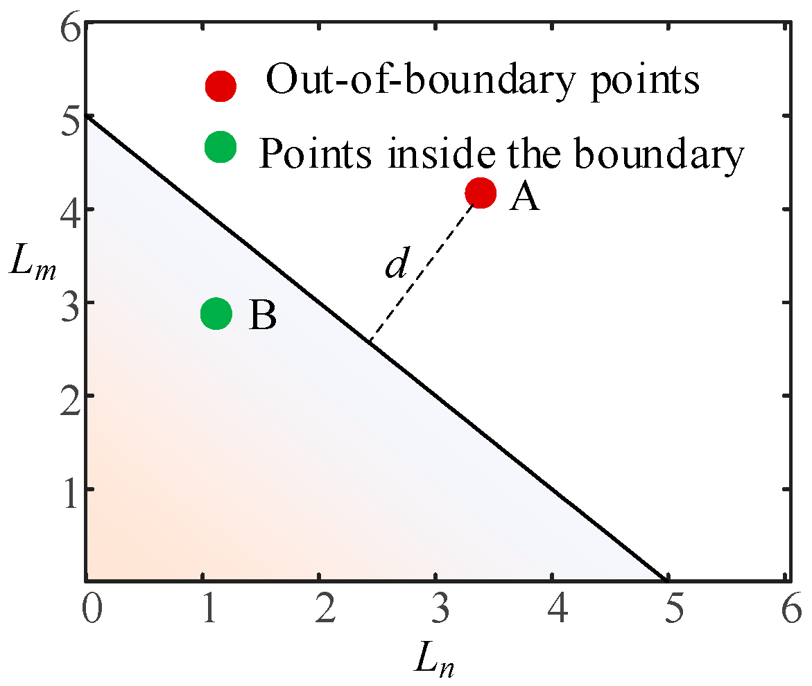
The proposed method effectively improves the efficiency of safety risk assessment calculations. By analyzing the mutual backup relationships between different devices and pipelines and constructing the DES safety boundary model, real-time online data assessment of operational status based on offline data are achieved. Compared to traditional online simulation methods, this method enhances computational efficiency.

(3)

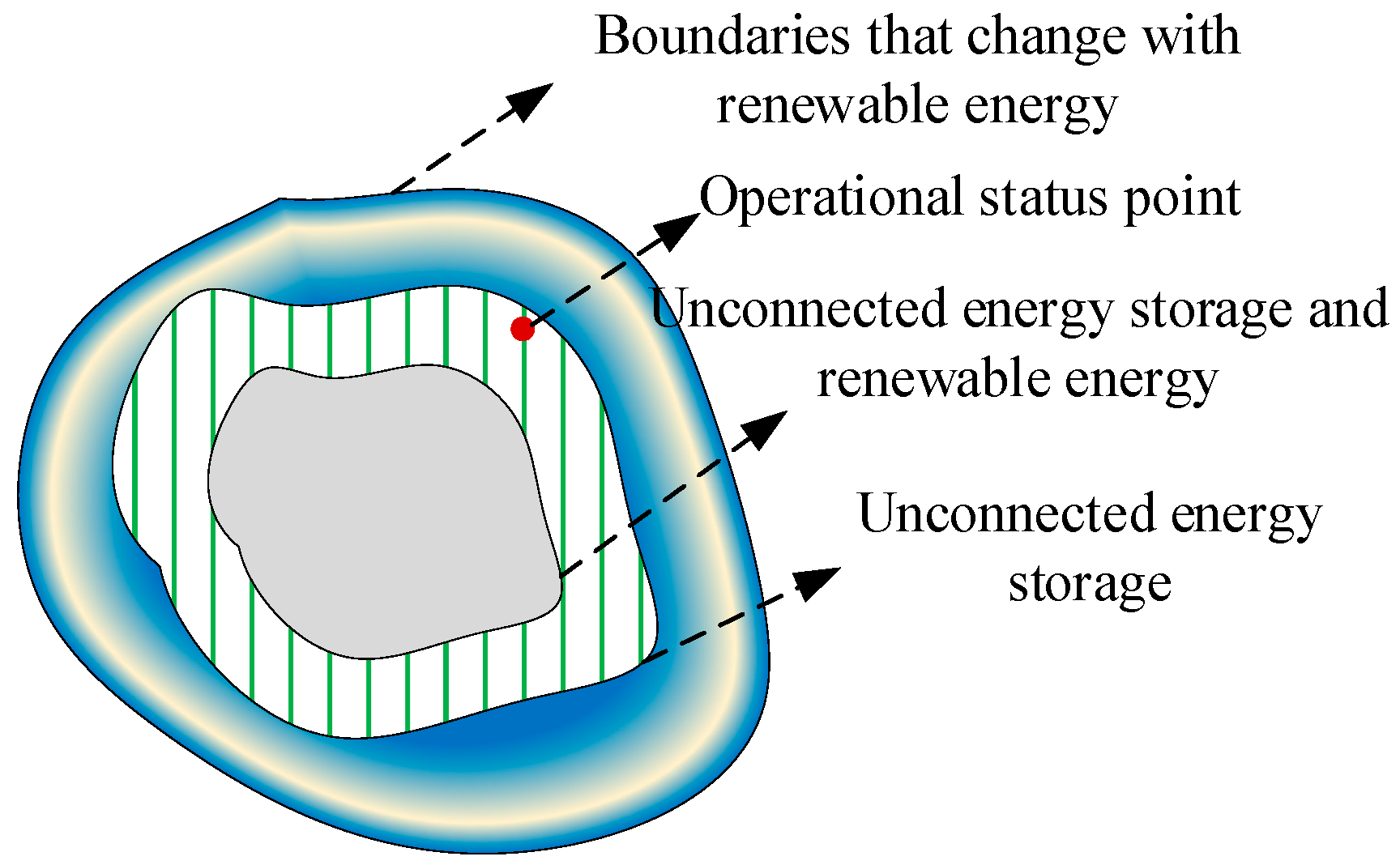
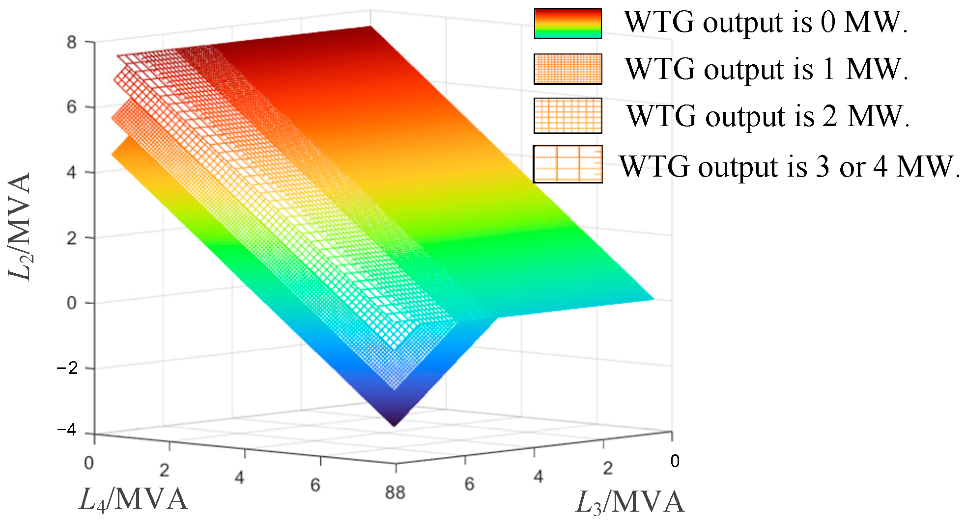
Variations in renewable energy output lead to changes in relevant equipment safety boundaries. Due to the stochastic nature of renewable energy output, the safety boundaries of related equipment relying on renewable energy as backup power become uncertain. However, this uncertainty is also constrained by the network structure at connection points.

(4)

The real-time calculation method for equipment failure probabilities proposed in this paper better matches actual equipment conditions. By considering the multi-risk characteristics of equipment health status, weather conditions, and other fault sources, a multi-risk source-based equipment failure probability model is constructed, making it more aligned with actual equipment conditions. Algorithm analysis demonstrates that the proposed method accurately quantifies the operational risks of energy stations.

(5)

For high-risk nodes, an energy storage optimization response strategy considering both economic and safety aspects is proposed, effectively reducing energy storage configuration costs and enhancing the operational safety and reliability of energy stations. This provides a reference for the planning and operation of energy stations.

(6)

In the future, more in-depth consideration will be given to safety risk response strategies and their application in practical engineering to validate their correctness.

References

1. Jiang, F.; Peng, X.; Tu, C.; Guo, Q.; Deng, J.; Dai, F. An improved hybrid parallel compensator for enhancing PV power transfer capability. IEEE Trans. Ind. Electron. 2021, 69, 11132–11143. [Google Scholar] [CrossRef]
2. Jiang, F.; Tu, C.; Guo, Q.; Shuai, Z.; He, X.; He, J. Dual-functional dynamic voltage restorer to limit fault current. IEEE Trans. Ind. Electron. 2018, 66, 5300–5309. [Google Scholar] [CrossRef]
3. Liang, X.; Jiang, F.; Peng, X.; Xiong, L.; Jiang, Y.; Gautam, S.; Li, Z. Improved Hybrid Reactive Power Compensation System Based on FC and STATCOM and Its Control Method. Chin. J. Electr. Eng. 2022, 8, 29–41. [Google Scholar] [CrossRef]
4. Qiu, Y.; Li, Q.; Ai, Y.; Chen, W.; Benbouzid, M.; Liu, S.; Gao, F. Two-stage distributionally robust optimization-based coordinated scheduling of integrated energy system with electricity-hydrogen hybrid energy storage. Prot. Control. Mod. Power Syst. 2023, 81, 33. [Google Scholar] [CrossRef]
5. Negnevitsky, M.; Nguyen, D.H.; Piekutowski, M. Risk assessment for power system operation planning with high wind power penetration. IEEE Trans. Power Syst. 2014, 30, 1359–1368. [Google Scholar] [CrossRef]
6. Li, X.; Zhang, X.; Wu, L.; Lu, P.; Zhang, S.H. Transmission line overload risk assessment for power systems with wind and load-power generation correlation. IEEE Trans. Smart Grid 2015, 6, 1233–1242. [Google Scholar] [CrossRef]
7. Luo, J.; Li, H.; Wang, S. A quantitative reliability assessment and risk quantification method for microgrids considering supply and demand uncertainties. Appl. Energy 2022, 328, 120130. [Google Scholar] [CrossRef]
8. Laowanitwattana, J.; Uatrongjit, S. Probabilistic power flow analysis based on partial least square and arbitrary polynomial chaos expansion. IEEE Trans. Power Syst. 2021, 37, 1461–1470. [Google Scholar] [CrossRef]
9. Xia, S.; Song, L.; Wu, Y.; Ma, Z.J.; Jing, J.P.; Ding, Z.H.; Li, G.Y. An integrated LHS–CD approach for power system security risk assessment with consideration of source–network and load uncertainties. Processes 2019, 7, 900. [Google Scholar] [CrossRef]
10. Ye, K.; Zhao, J.; Zhang, H.; Zhang, Y.C. Data-driven probabilistic voltage risk assessment of miniwecc system with uncertain PVs and wind generations using realistic data. IEEE Trans. Power Syst. 2022, 37, 4121–4124. [Google Scholar] [CrossRef]
11. Urbanik, M.; Tchórzewska-Cieślak, B.; Pietrucha-Urbanik, K. Analysis of the safety of functioning gas pipelines in terms of the occurrence of failures. Energies 2019, 12, 3228. [Google Scholar] [CrossRef]
12. Nemet, A.; Klemeš, J.J.; Moon, I.; Kravanja, Z. Safety analysis embedded in heat exchanger network synthesis. Comput. Chem. Eng. 2017, 107, 357–380. [Google Scholar] [CrossRef]
13. Cao, M.; Shao, C.; Hu, B.; Xie, K.G.; Li, W.Y.; Peng, L.B.; Zhang, W.X. Reliability assessment of integrated energy systems considering emergency dispatch based on dynamic optimal energy flow. IEEE Trans. Sustain. Energy 2021, 13, 290–301. [Google Scholar] [CrossRef]
14. Mu, Y.; Wang, C.; Cao, Y.; Jia, H.J.; Zhang, Q.Z.; Yu, X.D. A CVAR-based risk assessment method for park-level integrated energy system considering the uncertainties and correlation of energy prices. Energy 2022, 247, 123549. [Google Scholar] [CrossRef]
15. Wang, C.; Yan, C.; Li, G.; Liu, S.Y.; Bie, Z.H. Risk assessment of integrated electricity and heat system with independent energy operators based on Stackelberg game. Energy 2020, 198, 117349. [Google Scholar] [CrossRef]
16. Zhang, Y.; Yang, Z.; Ji, X.; Zhang, X.; Yu, Z.H.; Wu, F.C. Robust optimization of the active distribution network involving risk assessment. Front. Energy Res. 2022, 10, 963576. [Google Scholar] [CrossRef]
17. Xie, H.; Chen, H.; Deng, X.; Zhang, P.; Sun, Q. Electric-gas integrated energy system operational risk assessment based on improved k-means clustering technology and semi-invariant method. Proc. CSEE 2020, 40, 59–69. [Google Scholar] [CrossRef]
18. Wang, D.; Li, S.; Jia, H.; Xiao, J.; Guo, Y. Research on interval security region of regional integrated energy system integrated with renewable energy sources, part I: Concepts, modeling and dimension reduction observation. Proc. CSEE 2022, 42, 3188–3204. [Google Scholar] [CrossRef]
19. Chen, S.; Wei, Z.; Sun, G.; Wei, W.; Wang, D. Convex hull based robust security region for electricity-gas integrated energy systems. IEEE Trans. Power Syst. 2018, 34, 1740–1748. [Google Scholar] [CrossRef]
20. Shi, J.; Wang, Y.; Fu, R.; Zhang, J. Operating strategy for local-area energy systems integration considering uncertainty of supply-side and demand-side under conditional value-at-risk assessment. Sustainability 2017, 9, 1655. [Google Scholar] [CrossRef]
21. Zong, X.; Yuan, Y. Two-stage robust optimization of regional integrated energy systems considering uncertainties of distributed energy stations. Front. Energy Res. 2023, 11, 1135056. [Google Scholar] [CrossRef]
22. Cherdantseva, Y.; Burnap, P.; Blyth, A.; Eden, P.; Jones, K.; Soulsby, H.; Stoddart, K. A review of cyber security risk assessment methods for SCADA systems. Comput. Secur. 2016, 56, 1–27. [Google Scholar] [CrossRef]
23. Xiao, J.; Lin, X.; Jiao, H.; Song, C.; Zhou, H.; Zu, G.; Wang, D. Model, calculation, and application of available supply capability for distribution systems. Appl. Energy 2023, 348, 121489. [Google Scholar] [CrossRef]
24. Liu, L.; Wang, D.; Hou, K.; Jia, H.J.; Li, S.Y. Region model and application of regional integrated energy system security analysis. Appl. Energy 2020, 260, 114268. [Google Scholar] [CrossRef]
25. Zhou, B.; Fang, J.; Ai, X.; Yao, W.; Chen, Z.; Wen, J. Pyramidal approximation for power flow and optimal power flow. IET Gener. Transm. Distrib. 2020, 14, 3774–3782. [Google Scholar] [CrossRef]
26. Ding, T.; Jia, W.; Shahidehpour, M. A convex energy-like function for reliable gas flow solutions in gas transmission systems. IEEE Trans. Power Syst. 2021, 36, 4876–4879. [Google Scholar] [CrossRef]
27. Gomariz, F.P.; López, J.M.C.; Munoz, F.D. An analysis of low flow for solar thermal system for water heating. Sol. Energy 2019, 179, 67–73. [Google Scholar] [CrossRef]
28. Zhang, S.; Cheng, H.; Li, K.; Tai, N.; Wang, D.; Li, F. Multi-objective distributed generation planning in distribution network considering correlations among uncertainties. Appl. Energy 2018, 226, 743–755. [Google Scholar] [CrossRef]
29. Ren, Z.; Yan, W.; Zhao, X.; Li, W.; Yu, J. Chronological probability model of photovoltaic generation. IEEE Trans. Power Syst. 2013, 29, 1077–1088. [Google Scholar] [CrossRef]
30. Shi, C.; Ning, X.; Sun, Z.; Kang, C.; Du, Y.; Ma, G. Quantitative risk assessment of distribution network based on real-time health index of equipment. High Volt. Eng. 2018, 44, 534–540. [Google Scholar] [CrossRef]
31. Brown, R.E.; Frimpong, G.; Willis, H.L. Failure Rate Modeling Using Equipment Inspection Data. IEEE Trans. Power Syst. 2004, 19, 782–787. [Google Scholar] [CrossRef]
32. Wang, Y.; Chen, L.; Yao, M.; Li, X. Evaluating weather influences on transmission line failure rate based on scarce fault records via a bi-layer clustering technique. IET Gener. Transm. Distrib. 2019, 13, 5305–5312. [Google Scholar] [CrossRef]
33. Zhang, X.; Zheng, X.; Cheng, R.; Qiu, J.; Jin, Y. A competitive mechanism based multi-objective particle swarm optimizer with fast convergence. Inf. Sci. 2018, 427, 63–76. [Google Scholar] [CrossRef]
34. Guo, Y.; Wang, D.; Li, S.; Jia, H.; Li, J.; Zheng, Y.; Yang, Z. Optimal allocation of energy storage in regional integrated energy system based on security region. Power Syst. Technol. 2022, 46, 604–612. [Google Scholar] [CrossRef]
Figure 1. Schematic diagram of a network of distributed energy stations.
Sustainability 15 13741 g001
Figure 2. Schematic diagram of a distributed energy station.
Sustainability 15 13741 g002
Figure 3. The relationship between the operating point and the security boundary.
Sustainability 15 13741 g003
Figure 4. Schematic diagram of the impact of energy storage on security boundaries.
Sustainability 15 13741 g004
Figure 5. Security risk assessment and improvement strategy.
Sustainability 15 13741 g005
Figure 6. Power equipment boundary. (a) (T1, T2) failure condition; (b) CHP unit failure condition.
Sustainability 15 13741 g006
Figure 7. Security boundary of thermal and gas equipment. (a) (CHP, GB) failure condition; (b) (C1, C2) unit failure.
Sustainability 15 13741 g007
Figure 8. Power line security boundary. (a) L2 security boundary; (b) L4 security boundary.
Sustainability 15 13741 g008
Figure 9. Thermal pipeline security boundary.
Sustainability 15 13741 g009
Figure 10. Equipment security boundary under new energy access. (a) T1 security boundary; (b) T4 security boundary.
Sustainability 15 13741 g010
Figure 11. L2 security boundary under new energy access.
Sustainability 15 13741 g011
Figure 12. Energy storage optimization configuration scheme set to the Pareto frontier.
Sustainability 15 13741 g012