Fast and Robust State Estimation for Active Distribution Networks Considering Measurement Data Fusion and Network Topology Changes

Abstract

With the integration of distributed generations (DGs), distribution networks are being transformed into active distribution networks (ADNs). Due to ADNs‘ complex operational scenarios, massive data, and fast-changing network topologies, traditional state-estimation (SE) methods are inadequate to meet the requirements of computational accuracy, computational speed, and robustness. Aiming at the SE of ADNs, this paper proposes a data-driven and classic-model-integrated SE method, which uses an SE neural network (NN) to perform an initial estimation, and then uses linear SE to refine the estimation. It applies PMU and SCADA data fusion and is robust to noise and ADN topology changes. The simulations on the IEEE standard system verify that the proposed method is superior to traditional SE methods in terms of estimation accuracy, calculation speed, and robustness. This study provides ADNS with a new effective estimation scheme, which is of great significance in the context of promoting the development of renewable energy.

1. Introduction

With the rapid integration of DGs [1,2,3,4,5], distribution networks are being transformed into active distribution networks (ADNs) which have more complex structures and put forward higher requirements for monitoring and control [6,7]. To ensure the secure and stable operation of the ADN, it is necessary to efficiently and accurately monitor the system states in real time. So, it is important to study the state estimation (SE) of ADNs.

At present, the traditional SE models are mostly based on the weighted least square (WLS) method, which has been widely used in different scenarios for power systems and derived from many different branches [8]. Considering the characteristics of distribution networks, such as radial structure, a large number of network nodes, and low coverage of measurement configurations, various methods of SE in DN, including the nodal-voltage method [9,10,11], branch current method [12,13,14], and branch power method [15,16,17] have been proposed. However, the establishment of WLS theory relies on the assumption that the measurement noise obeys Gaussian distribution, and the estimation accuracy of WLS will be greatly affected if there are non-Gaussian noisy or significant deviation data (hereinafter referred to as bad measurement) in power grids. For this reason, robust SE methods with nonquadratic estimation criteria have been proposed, such as weighted least absolute value (WLAV) estimation [18,19], Huber-M estimation [20,21], and exponential objective function estimation [22,23]. In addition, to improve the computational accuracy of SE using the phasor measurement unit (PMU), SE methods that combine PMU and supervisory control and data acquisition (SCADA) measurements have been proposed, including linear SE by incorporating SCADA into PMU [24,25], nonlinear SE by incorporating PMU into SCADA [26], and two-stage models combining linear and nonlinear [27,28]. The above research provides a rich reference for SE in ADN. However, due to the complexity of multisource data types and frequent changes in network topology in ADN, traditional models have the following limitations.

First, traditional SE methods have difficulty simultaneously satisfying the requirements of robustness and fast computational speed. These methods typically rely on the system’s topology and measurements. So, incorrect topology and measurements will result in significant estimation biases and even cause the model’s failure of convergence. To enhance algorithm robustness, methods such as bad measurement detection and robust computation have been proposed. However, these methods are computationally complex and time-consuming, rendering them unable to meet the requirements of ADNs. With the increasing penetration of DGs, the numbers of operating states and load fluctuations in DN are significantly increased. Traditional SE is no longer capable of simultaneously meeting the requirements of robustness and speed.

Second, traditional SE methods have not achieved the fusion of PMU and SCADA data when performing the estimation. On the one hand, PMU and SCADA data have inconsistent updating cycles [29], whereas PMU data has a much higher updating frequency. Existing linear and nonlinear fusion models typically perform the fusion calculation only at the time instants with both PMU and SCADA updates, which does not fully leverage the PMU data [30]. On the other hand, some works attempted to generate pseudo-SCADA measurements for time instants with only the PMU data. However, pseudo-measurements suffer from low accuracy and difficult parameter configuration and are highly influenced by system states [28,31,32], leading to unstable estimations. The high sampling speed and accuracy of PMUs make it possible to enhance the frequency and accuracy of SE. So, there is an urgent need for more effective PMU–SCADA fusion schemes.

Thanks to the rich measurement data in ADNs, data-driven SE has attracted attention in recent years [33,34,35,36,37,38]. Refs. [23,24,25,26,27,28,29,30,31,32,33,34,35] performed robust SE based on deep NN. Ref. [36] used convolutional NNs and developed a data-fusion SE method. Refs. [37,38] used NNs for identifying DN topology. However, these methods still have shortcomings when performing SE of ADNs: (1) they only consider preknown bad measurement and have poor SE performances under random noises [33,34,35], (2) they neglect ADN’s topology changes and have low SE accuracy under different topologies [37,38], and (3) they fail to achieve a proper fusion of PMU and SCADA data, as discussed above [36].

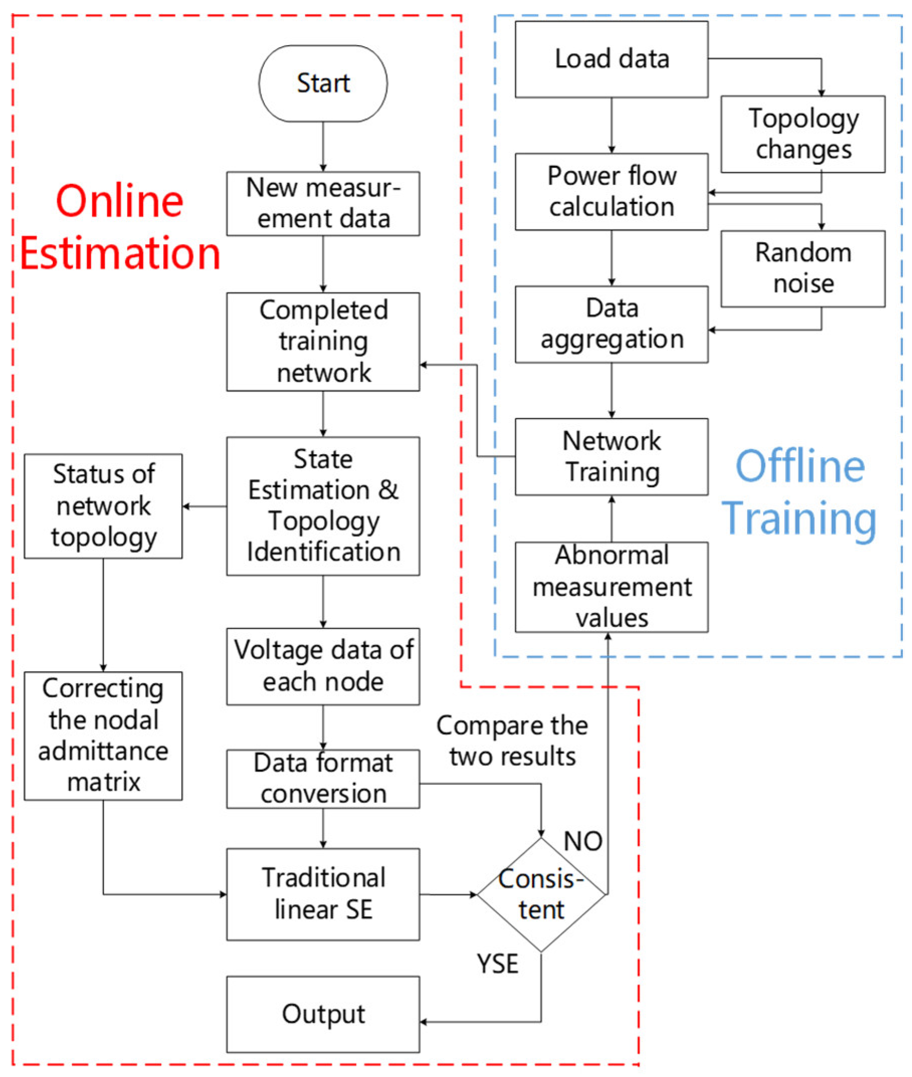
Considering this research gap, this paper proposes a fast and robust SE for ADNs, which performs PMU and SCADA data fusion and is adaptive to ADN’s topology changes. The contributions are threefold:

(1)

To address the issues of low accuracy and poor robustness in the SE of ADNs, this paper proposes a data-driven and classic model integrated fast robust SE model (FRSEM). It firstly constructs a multioutput NN for state pre-estimation, which directly associates the measured data with the true state values. Then, it corrects the NN outputs by using a linear SE model and increases the data redundancy for the SE. This not only enhances the SE accuracy but also greatly enhances the robustness in the cases of high-level noise and random topological changes of ADNs.

(2)

Aiming at a proper fusion of PMU and SCADA data, the proposed model includes different combinations of measurements during the NN’s training. The obtained NN can perform SE using SCADA data, PMU data, and the fused PMU and SCADA data, respectively. Even under scenarios with inadequate PMU measurements, the proposed model can still utilize PMU data for SE, which significantly reduces the time interval between two estimations and achieves real-time estimation.

(3)

In terms of estimation speed, due to the elimination of iterations, the proposed FRSEM has a faster computation speed compared to traditional methods. As verified by simulations, it is six times faster than the WLS method.

The remainder of the paper is organized as follows. Section 2 introduces the overall framework of the proposed FRSEM. The NN and its offline training are discussed in Section 3. Based on the NN’s outputs, The linear estimation is conducted in Section 4. Section 5 provides the simulation. Finally, Section 6 concludes the paper.

2. Framework of the Proposed Model

Figure 1 shows the overall structure of the proposed SE approach. In this paper, the proposed FRSEM for ADNs is proposed based on traditional linear SE and NN. Firstly, the initial estimation of the measurement data is performed by NN to obtain the relatively accurate SE value of the system; then, the relatively accurate SE value is fused with the PMU measurement data for linear SE to further correct the estimate and obtain the accurate state value. As shown in Figure 1, the model is divided into two stages: offline training and online estimation.

(1)

Offline Training: ① Real load data is used as the base data, combined with random factors such as load fluctuations, DG outputs, and topological changes to generate load data. The load flow values are then calculated, and noise is added to generate a measurement dataset for training. ② The SE network is designed based on traditional SE and topology identification methods; it consists of five feature-extraction layers and three output layers. The input to the network is measurement data, and the output includes node voltage magnitude, phase angle, and the system’s topological structure. ③ The network is trained using the dataset;

(2)

Online Estimation: ① The measurement data is transmitted to the trained network for estimation. The voltage magnitude and phase angle estimated by the network are converted, and the node admittance matrix is adjusted based on the topological output. ② Linear SE, whose inputs are PMU data, network estimation values, and the adjusted node admittance matrix, is performed to obtain accurate state values. ③ The linear SE values are compared with the NN’s output-voltage values. If there is a significant difference, the corresponding measurement value is reentered into the network for training.

3. Neural Network Design and Training in the SE of ADNs

This section discusses the NN model and its offline training in the SE, which addresses the issues of bad measurement interference, data fusion, and topological changes. Among them, the hyperparameters, such as the number of hidden layers and learning rate, are the optimal results obtained after repeated training many times.

3.1. NN Design

To achieve SE and topology identification, this paper designs a multioutput SE neural network (MSENN) based on the input–output characteristics and internal mechanisms of traditional methods. The model takes measurement data from various nodes in the distribution network as the input (1) and directly obtains the state parameters (voltage magnitude and phase angle) of each node and the network’s topological status through network computation (2). The specific design of the network is as follows.

$$X={\left[\begin{array}{ccc}{x}_1& \cdots & x_m\end{array}\right]}^{\mathrm{T}}$$

(1)

$$Y=\left[\begin{array}{c}{Y}^t\\ Y^{\alpha }\\ Y^{\theta }\end{array}\right]\cdots \cdots \cdots \left\{\begin{array}{l}{Y}^t={\left[\begin{array}{ccc}{t}_1& \cdots & t_p\end{array}\right]}^{\mathrm{T}}\\ Y^{\alpha }={\left[\begin{array}{ccc}{y^{\alpha }}_1& \cdots & {y^{\alpha }}_n\end{array}\right]}^{\mathrm{T}}\\ Y^{\theta }={\left[\begin{array}{ccc}{y^{\theta }}_1& \cdots & {y^{\theta }}_n\end{array}\right]}^{\mathrm{T}}\end{array}\right.$$

(2)

where, $X$ represents the input matrix of the network, $x$ represents the measurement values, and $m$ is the total number of measurements. $Y$ represents the output matrix of the network, and $Y^t$ represents the binary matrix indicating the topological status. $t_x$ represents the probability of the result being the $x$th topological structure. $p$ represents the number of topological states the system can have. $Y^{\alpha }$ represents the output-voltage magnitude matrix, $y^{\alpha }$ represents the voltage magnitude, $Y^{\theta }$ represents the output-node voltage vector, $y^{\theta }$ represents the node phase angle (in degrees), and $n$ represents the number of nodes.

(1)

Network Architecture and Activation Functions

Referring to the existing research, the layers of the state-estimation neural network are mostly between three and six. On this basis, this paper compares the neural network with three to six layers, and the results are shown in Appendix A. In addition, because the functional characteristics of the three outputs are not consistent, the network is designed in the form of hierarchical optimization. Firstly, a common layer network is used to extract the global characteristics of the measurement data, and, then, independent network layers are designed for different problems to achieve functional differentiation. As shown in Figure 2, the network consists of one input layer, five feature-extraction layers, and three output layers. Each layer is discussed as follows:

• Input layer: This layer receives the input matrix $X$ which contains the measurement values;
• Feature-extraction layers 1–2: These layers extract the overall features of the measurement data. Since the input can have both positive and negative values, the leaky ReLU activation function is used to ensure comprehensive feature extraction;
• Feature-extraction layer 3: This layer extracts the topological information from the overall features and uses the ReLU activation function to confine the output within the non-negative range;
• Feature-extraction layer 4: This layer extracts the voltage-magnitude information from the overall features. Since the voltage magnitudes of the system nodes typically fluctuate around one, the tanh activation function is used to limit the output magnitudes within the range of one;
• Feature-extraction layer 5: This layer extracts the voltage phase angle information and uses the leaky ReLU activation function to output phase angles within the range of [−180, 180];
• Output layer 1: This layer outputs the topological states in the features using the softmax activation function;
• Output layers 2 and 3: These layers use the tanh and leaky ReLU activation functions, respectively, to output the voltage magnitudes and phase angles;

The detailed parameter settings for each layer are shown in

Table 1. NN parameters.

Layer Name	Layer Number	Type/Activation Function	Size
Input Layer	1	fc/	$m\times 512$
Feature Layer	1	fc/leaky-relu	$512\times 512$
	2	fc/leaky-relu	$512\times 512$
	3	fc/relu	$512\times 256$
	4	fc/tanh	$512\times 256$
	5	fc/leaky-relu	$512\times 256$
Output Layer	1	fc/softmax	$128\times p$
	2	fc/tanh	$256\times n$
	3	fc/leaky-relu	$256\times n$

. The number of neurons in each layer was also obtained experimentally, see Appendix A.

(2)

Loss Function

In MSENN, the distinction of the topological state belongs to the classification problem in traditional machine learning, while the estimation of voltage for each node belongs to the regression problem. Therefore, for these two different outputs, different types of loss functions need to be used for training. In terms of topology, the cross-entropy loss function is used to directly calculate the topological loss value. In terms of SE, the loss is set as the MSE between the network’s output of voltage magnitude/angle and corresponding true values, following the traditional WLS method used in SE. The magnitude of the three loss values is maintained at an order of magnitude during the training without loss imbalance impacting the network effect. So, the overall loss function of the network is obtained by directly summing, as shown in the following formula:

$${loss}^t=\sum _{i=1}^p{\widehat{t}}_i\log t_i$$

(3)

$${loss}^{\alpha }=\sum _{i=1}^n{\left({{\widehat{y}}^{\alpha }}_i-{y^{\alpha }}_i\right)}^2$$

(4)

$${loss}^{\theta }=\sum _{i=1}^n{\left({{\widehat{y}}^{\theta }}_i-{y^{\theta }}_i\right)}^2$$

(5)

$${loss}^{all}={loss}^t+{loss}^{\alpha }+{loss}^{\theta }$$

(6)

where, ${loss}^t$, ${loss}^{\alpha }$, and ${loss}^{\theta }$ are the losses of topological, voltage magnitude, and angle, respectively, and ${loss}^{all}$ is the overall loss of the network. ${\widehat{t}}_i$, ${{\widehat{y}}^{\alpha }}_i$ and ${{\widehat{y}}^{\theta }}_i$ are the true values of topological state, voltage magnitude, and angle, respectively, of node $i$.

3.2. Data Set Generation

MSENN’s generalization requires historical measurement data. To obtain those data, reference [39] replaces the historical measurement data with noisy power-flow measurements under different load conditions. The actual load data for a week in a region of Belgium [40] are averaged, and, then, the true load curve is normalized to 0~1 to obtain the baseline daily load curve as shown in Figure 3 (where one day has 96 time instants with 15 min intervals). Gaussian noise with a standard deviation of 5% is added to generate the actual injected power at each node. A power-flow calculation was carried out through Matpower [41] to obtain the real value of voltage magnitude and angle, injected power, and line power at each ADN node. On this basis, measurement noise with normal distribution is added to generate SCADA and μPMU measurement data, where the error setting is the same as [42].

To address the situation that some of the measurement data in the distribution network may have significant deviations, noise with a mean value of ±50% and standard deviation of ±20% is added for 5% to 20% of each group’s data. These data are used as fault data to be cotrained with the network as a way to reduce the interference of deviant data on the results by using the filtering property of the NN. Generally, the measurement data with an error greater than ±6σ can be considered as fault data [43], and the error set in this paper has met the practical requirements. Regarding topological changes, when calculating the true values from each dataset, the topological structure is randomly modified to generate measurement data reflecting different network topologies. This simulates the topology changes that may occur in the distribution network and records the topology status of each data set.

In this study, for the case of inconsistent sampling periods between PMU and SCADA measurement data, a direct physical fusion approach is employed. At any given moment, the current monitoring data is directly fed into the network for estimation using the corresponding neural network neurons, while data not within the sampling period are inputted as zero to the corresponding neural network neurons. It should be noted that, apart from the aforementioned physical fusion, no additional data-processing techniques are applied to eliminate bad data. The purpose of using neural networks for estimation is to treat the neural network as a filter to mitigate interference caused by data anomalies, thereby enhancing the accuracy and performance of subsequent estimations.

Table 2. Five methods were used for combining SCADA and μPMU measurement data.

Method	Combination of SCADA and μPMU Data	Usage
1	${\left[\begin{array}{ccc}{x^{\mathrm{S}}}_1& \cdots & {x^{\mathrm{S}}}_{J^{ 1\ast }}\end{array}\hspace{1em},\hspace{1em}\begin{array}{ccc}{x^{\mathrm{P}}}_1& \dots & {x^{\mathrm{P}}}_{K^{ 2\ast }}\end{array}\right]}^{\mathrm{T}}$	Training
2	${\left[\begin{array}{ccc}0& \cdots & 0\end{array}\hspace{1em},\hspace{1em}\begin{array}{ccc}{x^{\mathrm{P}}}_1& \dots & {x^{\mathrm{P}}}_K\end{array}\right]}^{\mathrm{T}}$	Training
3	${\left[\begin{array}{ccc}0& \cdots & 0\end{array}\hspace{1em},\hspace{1em}\begin{array}{ccc}{x^{\mathrm{P}}}_1& \dots & {x^{\mathrm{P}}}_K\end{array}\right]}^{\mathrm{T}}\times L$	Training and Validation
4	${\left[\begin{array}{ccc}{{x^{\mathrm{S}}}_1}^{ 3\ast }& \cdots & {x^{\mathrm{S}}}_J\end{array}\hspace{1em},\hspace{1em}\begin{array}{ccc}0& \dots & 0\end{array}\right]}^{\mathrm{T}}\times L$	Training and Validation
5	${\left[\begin{array}{ccc}{x^{\mathrm{S}}}_1& \cdots & {x^{\mathrm{S}}}_J\end{array}\hspace{1em},\hspace{1em}\begin{array}{ccc}{{x^{\mathrm{P}}}_1}^{ 4\ast }& \dots & {x^{\mathrm{P}}}_K\end{array}\right]}^{\mathrm{T}}\times L^{ 5\ast }$	Training and Validation

^1* $J$ is the number of SCADA measurement data, ^2* $K$ is the number of μPMU measurement data, ^3* $x^{\mathrm{S}}$ is the measured value of SCADA, ^4* $x^{\mathrm{P}}$ is the measured value of SCADA, and ^5* $L=\left[\begin{array}{ccc}{l}_1& \cdots & l_{J+K}\end{array}\right]$, $l_j=\left\{\begin{array}{cc}1& Has measurements j\\ 0& Does not have measurement j\end{array}\right.$, $J+K$ = m.

lists five methods used for combining SCADA and μPMU measurement data. On this basis, a training dataset of m×1 dimensions can be obtained. Among them, the role of combination methods 1 and 2 is mainly to enhance the global features learned by the network during the training process and accelerate the convergence speed and accuracy of the network. Combinations 3, 4, and 5 correspond to scenarios where the network contains only μPMU data, only SCADA data, or a combination of both, respectively.

The flow chart of the data generation is shown in Figure 4. All the measured data are combined to construct the data set. In this paper, 100 days of measured data are generated, and 9600 groups of data sets are combined for network training and testing.

3.3. NN Training

The data sets of 6000, 1200, and 2400 were taken as the training set, validation set, and test set of the training network, respectively, and the network was trained for 10 rounds using the Adam optimizer. Among them, the initial learning rate used for training was $5\times {10}^{-5}$, with a decay of 0.75 per round; the network was trained 600 iterations per round, with 10 sets of data input each time. Since the randomly added noise has sufficiently prevented the overfitting of the network, no regularization strategy is taken. The loss decay of the network training is given in Figure 5.

As can be seen from Figure 5, MSENN converges well on the dataset, while the two loss curves have the same trend, indicating that the network has strong generalization performance. Due to the different bad measurements randomly added for each training, the loss values continue to fluctuate in the later stage of the training.

4. Online State Estimation Based on Network Outputs

This section discusses the online SE. The output of MSENN is integrated with the μPMU data to perform linear SE. Section 4.1 discusses the pre-estimation of MSENN, and Section 4.2 describes the linear SE based on the network output.

4.1. Initial Estimate Based on MSENN

After training, the MSENN has acquired topology identification and SE capabilities. The measurement data to be estimated is combined according to the actual measurement configuration and fed into the network for preliminary estimation. Three types of outputs are obtained: topology status, voltage magnitude, and voltage phase. Each of these outputs is transformed.

(1)

Voltage-Magnitude Conversion

Due to the limitation of the tanh activation function used in the voltage-output layer, it cannot have output-voltage magnitudes greater than one. Therefore, in this paper, voltage values are normalized. To restore the actual system voltages, the following transformation equation is used:

$$Y^{\alpha \_ture}=\frac{{\left[\begin{array}{ccc}{y^{\alpha }}_1& \cdots & {y^{\alpha }}_n\end{array}\right]}^T}{{y^{\alpha }}_{max}}$$

(7)

where, $Y^{\alpha \_ture}$ is the voltage truth matrix, and ${y^{\alpha }}_{max}$ is the maximum voltage in the system.

(2) Voltage-Angle Conversion

The voltage phase output from the network is in degrees. To facilitate subsequent calculations, it can be converted to radians using the following transformation equation:

$$Y^{\theta \_ture}=\frac{{\left[\begin{array}{ccc}{y^{\theta }}_1& \cdots & {y^{\theta }}_n\end{array}\right]}^T}{180/\pi }$$

(8)

where, $Y^{\theta \_ture}$ is the voltage phase angle truth matrix.

(3)

Topology Conversion

The label value used for topology recognition training is a binary code encoded by one_hot, so the output of the network topology state information is first converted to one_hot with the same type as the label value, and, then, the node derivative matrix characterizing the distribution-network topology is matched according to the converted output.

$${Y^t}_{o\_h}={\langle \frac{{\left[\begin{array}{ccc}{t}_1& \cdots & t_p\end{array}\right]}^T}{Max\left(\begin{array}{ccc}{t}_1,& \cdots & ,t_p\end{array}\right)}\rangle }_1$$

(9)

$$Y^G=\left\{\begin{array}{c}{y^G}_1 ,\hspace{1em}{Y^t}_{o\_h}=2^1\\ \begin{array}{c}⋮\\ {y^G}_i,\hspace{1em}{Y^t}_{o\_h}=2^i\\ ⋮\end{array}\\ {y^G}_p ,\hspace{1em}{Y^t}_{o\_h}=2^p\end{array}\right.$$

(10)

where, $Max\left(.\right)$ returns the maximum value of the brackets, ${〈.〉}_1$ means that the non-1 elements of the matrix are set to zero and the matrix is converted to binary value, ${Y^t}_{o\_h}$ is the output corresponding to one_hot binary code, $y^G$ is the output node derivative matrix, and ${y^G}_i$ is the $i$-th node derivative matrix of the system.

4.2. Linear SE Based on the Fusion-Network Output

On the one hand, the estimation performance of MSENN is closely related to the quality of the training data. When the nature of the new input measurement data differs significantly from the training set, it becomes difficult to ensure the estimation performance of the network. On the other hand, in cases where the number of PMU configurations is limited, the linear observable region formed by the PMUs is finite and may not meet the requirements of SE. Therefore, referring to the traditional approach of treating nonlinear SE results as pseudo-measurements [33], this paper treats the outputs of MSENN as pseudo-measurements and combines them with the μPMU measurement data for linear SE. The network output complements the linear observable region, while the μPMU measurement data corrects the network output, further improving the SE accuracy of the system.

The fusion estimation includes three inputs: the output-voltage vector of MSENN, the measured voltage vector of μPMU, the measured current vector of μPMU, and one output: the estimated voltage vector. When the system network structure and parameters are given, the linear relationship between the inputs and outputs can be represented based on the relevant circuit and the system knowledge, as follows:

$${Z=\left[{\left[\begin{array}{c}U\\ {\theta }^u\end{array}\right]}_{MSENN}\hspace{1em}{\left[\begin{array}{c}U\\ {\theta }^u\end{array}\right]}_{\mu PMU}\hspace{1em}{\left[\begin{array}{c}I\\ {\theta }^i\end{array}\right]}_{\mu PMU}\right]}^T=H{\left[\begin{array}{c}U\\ \theta \end{array}\right]}_{SE}+\epsilon$$

(11)

where, $Z$ is the input measurement matrix, ${\left[\begin{array}{c}U\\ {\theta }^u\end{array}\right]}_{MSENN}$ is the MSENN output-voltage vector, ${\left[\begin{array}{c}U\\ {\theta }^u\end{array}\right]}_{\mu PMU}$ and ${\left[\begin{array}{c}I\\ {\theta }^i\end{array}\right]}_{\mu PMU}$ are the voltage and current vectors of μPMU measurements, ${\left[\begin{array}{c}U\\ \theta \end{array}\right]}_{SE}$ is the estimated voltage vector, $H$ is the conversion matrix, and $\epsilon$ is the error.

According to the Maximum Likelihood Estimation theorem [43], when the error is minimized, the likelihood of the estimated value being equal to the true values of the system is maximized. Therefore, the estimation can be transformed into a weighted least squares problem. The objective criterion of the basic WLS method is to minimize the weighted sum of squared differences between the computed values of measurement functions and their corresponding measured values. The optimization objective function is as follows:

$$J=min{\left(\epsilon \right)}^T{R}^{-1}(\epsilon )=min{\left(Z-H{\left[\begin{array}{c}U\\ \theta \end{array}\right]}_{SE}\right)}^T{R}^{-1}\left(Z-H{\left[\begin{array}{c}U\\ \theta \end{array}\right]}_{SE}\right)$$

(12)

where, $J$ is the minimum error sum of squares, and $R$ is the weight matrix.

According to the extreme value condition, it is obtained that:

$${\left[\begin{array}{c}U\\ \theta \end{array}\right]}_{est}={\left[H^{\mathrm{T}}{R}^{-1}H\right]}^{-1}{H}^T{R}^{-1}Z$$

(13)

where, ${\left[\begin{array}{c}U\\ \theta \end{array}\right]}_{est}$ is the SE result.

It is important to note that the fusion-estimation model mentioned here is still linear and can be solved without iteration; thus, it will not have a significant impact on the real-time performance of the overall estimation.

Finally, the analysis is conducted on the network output and SE output using voltage magnitude as the indicator, as shown in (14), where 1% is used as the index to make decisions in this paper.

$$J=Max({\sum }_{i=1}^n\left|{u_i}^{MSENN}-{u_i}^{SE}\right|)\times 100\%$$

(14)

where, $J$ is the decision indicator, ${u_i}^{MSENN}$ represents the voltage magnitude of the $i$-th node obtained from the converted network output, and ${u_i}^{SE}$ represents the voltage magnitude of the $i$-th node from the SE output.

5. Simulation and Analysis

To verify the performance of the proposed FRSEM, simulations on the IEEE 33 distribution system with DGs are conducted. Section 5.1 verifies the accuracy and robustness of the proposed model. Section 5.2 and Section 5.3 demonstrate the model’s performance in two scenarios—data fusion and topology changes. Section 5.4 performs a timeliness analysis of the model.

Figure 6 shows the studied distribution system, with 33 nodes and 37 lines. The load data for each node is sourced from MATPower. DGs with rated capacities of 400 kW, 500 kW, 350 kW, and 450 kW are connected to nodes 7, 10, 14, and 33, respectively. Referring to [44], the output range of the DGs is 0~1.5 times of rated capacities.

Table 3. The four ADN topologies were used in the simulation.

Topology	DG Output (%)	Disconnected Switch
1	0	7-8, 9-10, 14-15, 32-33, 25-29
2	50	7-8, 10-11, 13-14, 31-32, 25-29
3	100	7-8, 10-11, 14-15, 30-31, 25-29
4	150	7-8, 9-10, 14-15, 28-29, 18-33

lists four reconstructed networks with corresponding DG outputs.

In Section 5.1, measurement devices for node and branch power measurements are installed at all nodes and branches, respectively. Additionally, a voltage-magnitude measurement is installed at node 1 to provide reference voltage values for SE.

In Section 5.2 and Section 5.3, in addition to the aforementioned measurements, eight μPMUs are installed at nodes 3, 6, 10, 13, 17, 21, 25, and 29. These μPMUs provide synchronized voltage and current measurements.

The mean absolute error (MAE), mean relative error (MRE), and topology identification accuracy (TIA) are used as evaluation metrics for SE and topology identification accuracy, respectively. The formulas are as follows:

$$MAE={\sum }_1^{\widehat{t}}\left|v-\widehat{v}\right|/\widehat{t}$$

(15)

$$MRE=100\%\times {\sum }_1^{\widehat{t}}\frac{\left|v-\widehat{v}\right|}{\left|\widehat{v}\right|}/\widehat{t}$$

(16)

$$TIA=(t/\widehat{t})\times 100\%$$

(17)

where, $v$ is the estimated value, $\widehat{v}$ is the true value, $\widehat{t}$ is the total number of test-set groups (2400), and $t$ is the number of groups with correct topology estimation.

The simulation was performed on a personal computer equipped with an Intel(R) Core i7-12700 CPU and MATLAB 2022a environment. The computer has 64 GB of memory and Matpower version 4.01 installed. The simulation code was executed using the CPU.

5.1. Comparison of Estimation Accuracy and Robustness

SE simulation experiments are conducted using both the traditional WLS method and the proposed FRSEM method in two SCADA measurement scenarios with normal data and with bad measurement. The estimation accuracy and robustness are compared. The MAE for each node is shown in Figure 7, while the MAE and TIA of the system are presented in

Table 4. MAE and TIA of system.

Method	Magnitude MSE (pu)	Magnitude RAE %	Angle MSE (°)	Angle RAE %	TIA (%)
WLS + Normal Data	0.0210	1.88	0.0942	2.58	\
WLS + Bad Data	0.0337	3.43	0.0931	2.67	\
FRSEM + Normal Data	0.0029	0.29	0.0529	1.66	100
FRSEM + Bad Data	0.0031	0.3	0.0669	1.84	99.958

.

As can be seen from the graphs, WLS and FRSEM can obtain stable results in both scenarios, and the accuracy of each node in the same method and scenario is roughly consistent, staying within a relatively small fluctuation range. Under normal measurement conditions, the voltage-magnitude errors for WLS and FRSEM fluctuate around 0.0210 pu and 0.0029 pu respectively, while the voltage-angle errors fluctuate around 0.0942° and 0.0529°. The estimation performance of FRSEM significantly surpasses that of WLS, especially in terms of voltage-magnitude errors, which are almost an order of magnitude smaller than WLS. When introducing bad measurements into the measurements, the voltage-magnitude errors of the system in WLS show significant increases, while the voltage-angle errors exhibit larger fluctuations; but, the overall errors remain nearly unchanged. On the other hand, most nodes in FRSEM maintain unchanged voltage-magnitude errors, with only a few nodes showing minor increases. The voltage-angle errors of each node also experience some increases, but the overall phase-angle error is still much smaller than WLS. Additionally, FRSEM possesses the capability of topology identification, which is not present in conventional WLS. It accurately identifies the system’s topology in both scenarios.

The experiments demonstrate that FRSEM achieves higher estimation accuracy and robustness compared to WLS, confirming the expected results. This is because traditional WLS is essentially a probabilistic estimation model that relies on known measurement-error probability distributions to infer the most probable system-state distribution. The estimation accuracy is limited within a certain range due to fixed measurement-error sizes. Furthermore, when bad measurement disturbs the correct measurement-error distribution, the estimation accuracy decreases significantly. Unlike traditional WLS, the FRSEM proposed in this paper utilizes NNs as its core component. It directly trains the network using the true system states, establishing a stronger correlation between measurement values and true values. Moreover, the inherent filtering of NNs helps reduce the impact of bad measurement, resulting in better performance than traditional WLS in both scenarios.

5.2. Comparison of SE Accuracy under Fused Measurement Data

The estimation accuracy of the fusion of mixed measurements (including μPMU and SCADA) using WLS [9] and FRSEM in SE is compared. The comparison is conducted for two cases: one with both types of measurements and the other with only μPMU measurements. The results are shown in Figure 8 and

Table 5. MAE and TIA of system.

Method	Magnitude MSE (pu)	Magnitude RAE%	Angle MSE (°)	Angle RAE %	TIA (%)
WLS + SCADA + μPMU	0.0110	1.12	0.0944	2.86	\
FRSEM + μPMU	0.0024	0.24	0.0321	0.98	100
FRSEM + SCADA + μPMU	0.0021	0.22	0.0285	0.85	100

. It is noted that there are insufficient observable regions for the eight μPMUs to support estimation using WLS alone, so the results for WLS + μPMU are not included in the experimental results.

As shown in Figure 8, after introducing μPMU into the measurement, the voltage-magnitude errors in WLS exhibit significant fluctuations, while the voltage-magnitude errors at the μPMU-connected nodes are significantly reduced. The voltage-angle errors show some fluctuations but, overall, remain unchanged. On the other hand, FRSEM demonstrates a significant reduction in both voltage-magnitude and phase-angle errors, with the angle error at the μPMU-connected nodes almost reaching zero. Although the reduction in voltage-magnitude error of FRSEM is not as great as WLS, the voltage-magnitude errors at all nodes in FRSEM are still smaller than in WLS. Additionally, the results in the table demonstrate that, unlike WLS, FESEM can still perform SE even with insufficient μPMU measurements, and the missing SCADA measurements only cause slight accuracy degradation in the model.

Simulation results show that μPMU measurements significantly enhance the effectiveness of both methods, but the performance of FESEM proposed in this paper is more outstanding. Moreover, this method increases the SE usage scenario of μPMU measurement by supplementing the measurement data with NNs.

5.3. Comparison of SE Accuracy under ADN Topology Changes

To demonstrate the impact of topology changes on the estimation accuracy and highlight the necessity of correcting the topology state, this subsection compares the SE accuracy of WLS and FESEM before and after correcting the topology information (based on the topology state output by MSENN), respectively.

Each day is divided into 96 time instants (with 15 min intervals). The ADN topology changes at the 42nd and 50th time instants. The MAE is obtained as shown in Figure 9.

The results show that during the time of 0~42, there are no topology changes in the system, and the results obtained by both methods before and after topology correction completely overlap. However, after the topology changes occur at the 42nd and 50th time instants, correcting the topology leads to a significant reduction in errors. Among them, due to the existence of voltage-magnitude measurement data, the output-voltage magnitude is less sensitive to topology changes, and the reduction of angle error is more obvious [45,46]. In addition, topology changes in the results have a greater impact on the WLS because the network pre-estimation in the first stage of FESEM does not require topology information, and incorrect topology information only affects the process of linear SE, which uses μPMU measurements consisting entirely of voltage magnitude and angle. It greatly reduces the extent to which topology affects the estimation.

The above analysis indicates that using MSENN’s topology output to correct the network topology before estimation effectively enhances the SE accuracy under topology changes. This is particularly significant for distribution networks with frequent topology changes caused by DER integration.

5.4. Time-Sensitive Analysis

To verify the efficiency of the proposed method, the computation time for running both methods 100 times was calculated and compared. Additionally, to clarify the impact of the linear SE on the computation time and accuracy of FESEM, the computation time for the standalone MSENN was also included in the comparative experiment. The accuracy of each method is presented in

Table 6. Timeliness and accuracy analysis.

Method	Magnitude MSE (pu)	Magnitude RAE %	Angle MSE (°)	Angle RAE %	Time (s)
WLS	0.0115	1.17	0.0997	2.81	1.1798
FRSEM	0.0034	0.32	0.0329	1.01	0.1704
MSENN	0.0037	0.41	0.0786	2.11	0.0099

.

Compared to WLS, the proposed MSENN method in this study replaces the Newton–Raphson method with forward computation and backward propagation, and utilizes parallel computing instead of serial computing, resulting in significant speed advantages. Although the introduction of linear SE in FRSEM increases the computation time to some extent, the overall computation time is still much smaller than that of WLS. Both MSENN and FRSEM demonstrate better efficiency compared to the traditional WLS. In terms of overall accuracy, it can be observed that FRSEM achieves the highest accuracy among the three methods, but it is slower than MSENN. On the other hand, MSENN is the fastest in terms of computation speed but has slightly lower accuracy compared to FRSEM. Therefore, depending on different scenarios, it is possible to flexibly choose between the two methods to meet specific practical requirements.

5.5. Simulation on P&F 69 System

To further demonstrate the generality of the proposed method, this study conducted additional testing on the P&F 69 distribution system. The results are shown in Figure 10 and

Table 7. Comparison of two systems.

Method	Magnitude MSE (pu)	Magnitude RAE %	Angle MSE (°)	Angle RAE %	Time (s)
IEEE 33	0.0021	0.22	0.0285	0.85	1.1869
P&G 69	0.0023	0.27	0.0318	0.96	1.1934

below. Compared to the 33-node system, the accuracy fluctuates relatively more for each node, while the overall average accuracy remains almost unchanged. Additionally, due to the increased number of input measurements, the overall processing time has slightly increased.

6. Conclusions

This paper proposes a fast and robust state-estimation (SE) method for active distribution networks (ADN) that addresses the challenges of balancing robustness and computation speed in traditional SE, as well as the data-fusion issue between phasor measurement units (PMUs) and supervisory control and data acquisition (SCADA) systems. The proposed method achieves the following goals through simulations on an IEEE 33-node system with distributed energy resources (DER):

• Robust SE with high accuracy: Our method achieves higher accuracy than traditional methods, particularly in terms of voltage-magnitude accuracy. It exhibits strong robustness, minimizing the impact of bad measurements;
• Fusion of PMU and SCADA data: The accuracy and stability of fusing PMU and SCADA data are higher than traditional SE methods. The proposed method can perform high-precision SE, even with insufficient PMU measurements;
• Improved computation speed: The proposed method is significantly faster than the traditional method, enabling real-time estimation. It also reduces the influence of topology changes on estimation accuracy by modifying the neural network’s topology.

Moving forward, there are several potential avenues for future research in this field. It is crucial to shift our focus towards the perception and optimization of other unknown variables in ADN, such as nonelectrical quantity estimation and the optimization of auxiliary monitoring devices. By exploring these areas, we can further improve the overall performance and efficiency of ADN systems.

References

1. Huzaifa, M.; Hussain, A.; Haider, W.; Kazmi, S.A.A.; Ahmad, U.; Rehman, H.U. Optimal Planning Approaches under Various Seasonal Variations across an Active Distribution Grid Encapsulating Large-Scale Electrical Vehicle Fleets and Renewable Generation. Sustainability 2023, 15, 7499. [Google Scholar] [CrossRef]
2. Ngamroo, I.; Kotesakha, W.; Yoomak, S.; Ngaopitakkul, A. Characteristic Evaluation of Wind Power Distributed Generation Sizing in Distribution System. Sustainability 2023, 15, 5581. [Google Scholar] [CrossRef]
3. Kesheng, G.E.; Chen, H. Sitting and Sizing Method of Multi-objective Distributed Generation Considering Distribution Network Reliability. Hunan Electr. Power 2021, 3, 21–24+29. [Google Scholar]
4. Jiang, F.; Peng, X.; Tu, C.; Guo, Q.; Deng, J.; Dai, F. An improved hybrid parallel compensator for enhancing PV power transfer capability. IEEE Trans. Ind. Electron. 2022, 69, 11132–11143. [Google Scholar] [CrossRef]
5. Guo, Q.; Tu, C.; Jiang, F.; Zhu, R.; Ye, J.; Gao, J. An overview of series-connected power electronic converter with function extension strategies in the context of high-penetration of power electronics and renewables. Renew. Sustain. Energy Rev. 2022, 156, 11934. [Google Scholar] [CrossRef]
6. Hu, R.; Wang, W.; Wu, X.; Jing, L.; Ma, W. Three-stage Robust Voltage Control Method for Active Distribution Network with Soft Open Points. Gaodianya Jishu/High Volt. Eng. 2020, 46, 3752–3761. [Google Scholar] [CrossRef]
7. Qu, H.; Li, X.; Yang, L.; Huang, Y.; Wang, M.; Huang, J. Multi-objective Distribution Network Dynamic Reconfiguration and DG Control Considering Time Variation of Load and DG. Gaodianya Jishu/High Volt. Eng. 2019, 45, 873–881. [Google Scholar] [CrossRef]
8. Schweppe, F.C.; Wildes, J. Power system static state estimation, part I, part II and part III. IEEE Trans. Power Appar. Syst. 1970, 89, 120–135. [Google Scholar] [CrossRef]
9. Tengjh, L.; Liu, W.H.E. Distribution system state estimation. IEEE Transon. Power Syst. 1995, 10, 229–240. [Google Scholar]
10. Lin, W.-M.; Teng, J.H. State estimation for distribution systems with zero-injection constraints. IEEE Trans. Power Syst. 1996, 11, 518–524. [Google Scholar] [CrossRef]
11. Duan, J.-D.; Sun, Y.-K.; Yin, X.-G. Voltage stability’s online prediction using WAMS. Gaodianya Jishu/High Volt. Eng. 2009, 35, 1748–1752. [Google Scholar]
12. Baran, M.E.; Kelley, A.W. A branch-current-based state estimation method for distribution systems. IEEE Transon. Power Syst. 1995, 10, 483–491. [Google Scholar] [CrossRef]
13. Wang, H.; Schulz, N.N. A revised branch current-based distribution system state estimation algorithm and meter placement impact. IEEE Trans Power Syst. 2004, 19, 207–212. [Google Scholar] [CrossRef]
14. Yan, L.; Ai, X.; Wang, Y.; Zhao, K. A new method to lead PMU branch current measurement into nonlinear state estimation. Dianwang Jishu/Power Syst. Technol. 2014, 38, 2816–2821. [Google Scholar]
15. Ju, Y.; Wu, W.; Zhang, B. A new method for distribution state estimation accommodating current measurements. Zhongguo Dianji Gongcheng Xuebao/Proc. Chin. Soc. Electr. Eng. 2011, 31, 82–89. [Google Scholar]
16. Peng, Q.; Jiang, T.; Yang, Y.-H. State-estimation iteration algorithm of distribution network based on y-matrix equation. Zhongguo Dianji Gongcheng Xuebao/Proc. Chin. Soc. Electr. Eng. 2008, 28, 65–68. [Google Scholar]
17. Sun, H.; Zhang, B.; Xiang, N. A branch-power-based state estimation method for distribution systems. Autom. Electr. Power Syst. 1998, 22, 12–16. (In Chinese) [Google Scholar]
18. Yan, Q.; Wei, Z.; Sun, G.; Wang, C.; Sun, W. A robust WLAV state estimation based on multiple predictor-corrector interior point method. Dianwang Jishu/Power Syst. Technol. 2013, 37, 2194–2200. [Google Scholar]
19. Wei, H.; Sasaki, H.; Kubokawa, J.; Yokoyama, R. An interior point method for power system weighted nonlinear L/sub 1/norm static state estimation. IEEE Trans. Power Syst. 1998, 13, 617–623. [Google Scholar] [CrossRef]
20. Guo, W.; Shan, Y. M-estimation and its application in power system state estimation. Zhongguo Dianji Gongcheng Xuebao/Proc. Chin. Soc. Electr. Eng. 2000, 20, 26–31. [Google Scholar]
21. Mili, L.; Cheniae, M.G.; Vichare, N.S.; Rousseeuw, P.J. Robust state estimation based on projection statistics [of power systems]. IEEE Trans. Power Syst. 1996, 11, 1118–1127. [Google Scholar] [CrossRef]
22. Wu, W.; Guo, Y.; Zhang, B. A robust state estimation method with exponential objective function. Zhongguo Dianji Gongcheng Xuebao/Proc. Chin. Soc. Electr. Eng. 2011, 31, 67–71. [Google Scholar]
23. Fu, Y.; Chen, Y.; Yao, R.; Liu, F.; Mei, S.; Huang, L. A robust state estimation approach based on objective function of maximum exponential absolute value. Dianwang Jishu/Power Syst. Technol. 2013, 37, 3166–3171. [Google Scholar]
24. Wei, Z.-N.; Li, Y.-L.; Zheng, Y.-P. A Mixed Measurement-based Linear Dynamic State Estimation Algorithm for Power Systems. Autom. Electr. Power Syst. 2007, 31, 39–43. [Google Scholar]
25. Haozhong, C.; Qingshan, Y.; Yihua, W.; Jingsong, G. A state estimation method of power systems based on equivalent current measurement transformation. Autom. Electr. Power Syst. 2000, 24, 28–29. [Google Scholar]
26. Hong, Z.; Xue, Y.; Dexin, W. State Estimation Model with PMU Current Phasor Measurements. Autom Electr. Power Syst. 2004, 28, 37–40. [Google Scholar]
27. Yu, Q.-J.; Wang, X.-R.; You, J.-X.; Lan, P.-Q. EqualityConstraints Two-Step State Estimation Model Based on Phasor Measurements. Power Syst. Technol. 2007, 31, 8488. [Google Scholar]
28. Nuqui, R. State Estimation and Voltage Security Monitoring Using Synchronized Phasor Measurements. Ph.D. Thesis, Virginia Polytechnic Institute and State University, Blacksburg, VA, USA, 2001; pp. 1–206. [Google Scholar]
29. Hong-Xia, M. A Novel Power System State Estimation Method Based on Merging PMU-Measured Data into SCADA Data. Power Syst. Technol. 2008, 32, 44–49. [Google Scholar]
30. Zhao, H. Study on Phasor Measurements and DC Model in Power System State Estimation; Shandong University: Jinan, China, 2004. [Google Scholar]
31. Sinha, A.K.; Mondal, J.K. Dynamic state estimator using ANN based bus load prediction. IEEE Trans. Power Syst. 1999, 14, 1219–1225. [Google Scholar] [CrossRef]
32. You, J.-X.; Huang, B.; Guo, C.-X.; Cao, Y.-J. State estimation using SCADA and PMU mixed measurements. Gaodianya Jishu/High Volt. Eng. 2009, 35, 1765–1769. [Google Scholar]
33. Wang, Z.; Zhang, Y.; Ji, X.; Xu, B.; Yang, M.; Han, X. Robust State Estimation of Power System Based on Deep Learning and Kernel Ridge Regression. Gaodianya Jishu/High Volt. Eng. 2022, 48, 1332–1342. [Google Scholar] [CrossRef]
34. Hu, J.; Cao, D.; Hu, W.; Chen, J.; Chen, Z. Robust State Estimation Method for Distribution Network Based on Graph Neural Network Incorporating Topology Knowledge. Dianli Xitong Zidonghua/Autom. Electr. Power Syst. 2023, 47, 84–97. [Google Scholar] [CrossRef]
35. Yu, W.; Zhang, X.; Wei, Z.; Sun, G.; Zang, H.; Yang, Y.; Han, Y. Fast State Estimation for Power System Based on Deep Neural Network. Dianwang Jishu/Power Syst. Technol. 2021, 45, 2551–2559. [Google Scholar] [CrossRef]
36. Liu, X.; Zeng, X.; Huang, Y.; Dong, L.; Zhang, H.; Liu, D.; Wang, X.; Li, Y.; Deng, C. State Estimation Based on Particle Filtering and Convolutional Neural Networks for Power Systems. Dianwang Jishu/Power Syst. Technol. 2020, 44, 3361–3367. [Google Scholar] [CrossRef]
37. Pei, Y.; Qin, C.; Yu, Y. Online Topology Identification for Smart Distribution Grids Based on LightGBM and Deep Neural Networks. Tianjin Daxue Xuebao (Ziran Kexue Yu Gongcheng Jishu Ban)/J. Tianjin Univ. Sci. Technol. 2020, 53, 939–950. [Google Scholar] [CrossRef]
38. Pan, Y.; Qin, C. Identification Method for Distribution Network Topology Based on Two-stage Feature Selection and Gramian Angular Field. Dianli Xitong Zidonghua/Autom. Electr. Power Syst. 2022, 46, 170–177. [Google Scholar] [CrossRef]
39. Chen, Y.; Wang, Y.; Yang, Q. Real-time State Estimation Method for Distribution Networks Based on Spatial-temporal Feature Graph Convolution Network. Gaodianya Jishu/High Volt. Eng. 2021, 47, 2386–2395. [Google Scholar] [CrossRef]
40. Elia. Load and Load Forecast [DB/OL]. Available online: https://www.elia.be/en/grid-data/Load-and-Load-Forecasts (accessed on 21 March 2023).
41. Zimmerman, R.D.; Murillo-Sanchez, C.E.; Thomas, R.J. MATPOWER: Steady-State Operations, Planning, and Analysis Tools for Power Systems Research and Education. IEEE Trans. Power Syst. 2010, 26, 12–19. [Google Scholar] [CrossRef]
42. Li, C.; Liu, T.; Li, X.; Wu, X. Data fusion method of WAMS/SCADA hybrid measurements in power system state estimation. Gaodianya Jishu/High Volt. Eng. 2013, 39, 2686–2691. [Google Scholar]
43. Chen, Y.; Yu, E. Power System State Estimation; Science Press: Beijing, China, 2021. [Google Scholar]
44. Dorostkar-Ghamsari, M.R.; Fotuhi-Firuzabad, M.; Lehtonen, M.; Safdarian, A. Value of Distribution Network Reconfiguration in Presence of Renewable Energy Resources. IEEE Trans. Power Syst. 2015, 31, 1879–1888. [Google Scholar] [CrossRef]
45. Omer, L.; Harley, R.G.; Habetler, T.G. Bus admittance matrix estimation using phasor measurements. In Proceedings of the 2019 IEEE Power & Energy Society Innovative Smart Grid Technologies Conference (ISGT), Washington, DC, USA, 18–21 February 2019. [Google Scholar]
46. Gotti, D.; Amaris, H.; Ledesma, P. A Deep Neural Network Approach for Online Topology Identification in State Estimation. IEEE Trans. Power Syst. 2021, 36, 5824–5833. [Google Scholar] [CrossRef]
Figure 1. Framework of the Proposed Model.
Sustainability 15 13800 g001
Figure 2. MSENN structure diagram.
Sustainability 15 13800 g002
Figure 3. Base load curve.
Sustainability 15 13800 g003
Figure 4. General flow chart of data generation.
Sustainability 15 13800 g004
Figure 5. Training loss drop of the NN.
Sustainability 15 13800 g005
Figure 6. Studied Distribution system.
Sustainability 15 13800 g006
Figure 7. Average absolute value error of each node.
Sustainability 15 13800 g007
Figure 8. Average absolute value error of each node.
Sustainability 15 13800 g008
Figure 9. The variations of MAEs of the ADN nodes.
Sustainability 15 13800 g009
Figure 10. Average absolute value error of each node.
Sustainability 15 13800 g010