Article

Application of a Hyperspectral Remote Sensing Model for the Inversion of Nickel Content in Urban Soil

1
College of Geographical Science and Tourism, Xinjiang Normal University, Urumqi 830054, China
2
Xinjiang Laboratory of Arid Zone Lake Environment and Resources, Xinjiang Normal University, Urumqi 830054, China
3
School of Geography and Tourism, Shaanxi Normal University, Xi’an 710119, China
*
Author to whom correspondence should be addressed.
Sustainability 2023, 15(18), 13948; https://doi.org/10.3390/su151813948
Submission received: 22 August 2023 / Revised: 14 September 2023 / Accepted: 15 September 2023 / Published: 20 September 2023

Abstract

:
Hyperspectral remote sensing technology can provide a rapid and nondestructive method for soil nickel (Ni) content detection. In order to select a high-effective method for estimating the soil Ni content using a hyperspectral remote sensing technique, 88 soil samples were collected in Urumqi, northwest China, to obtain Ni contents and related hyperspectral data. At first, 12 spectral transformations were used for the original spectral data. Then, Pearson’s correlation coefficient analysis (PCC) and the CARS method were used for selecting important wavelengths. Finally, partial least squares regression (PLSR), random forest regression (RFR) and support vector machine regression (SVMR) models were used to establish the hyperspectral inversion models of the Ni content in the soil using the important wavelengths. The coefficient of determination (R2), root mean square error (RMSE), mean absolute error (MAE), and residual prediction deviation (RPD) were selected to evaluate the inversion effects of the models. The results indicated that using the PCC and CARS method for the original and transformed wavebands can effectively improve the correlations between the spectral data and Ni content of the soil in the study area. The random forest regression model, based on the first-order differentiation of the reciprocal (RTFD–RFR), was more stable and had the best inversion effects, with the highest predictive ability (R2 = 0.866, RMSE = 1.321, MAE = 0.986, RPD = 2.210) for determining the Ni content in the soil. The RTFD–RFR methods can be used as a means of the inversion of the Ni content in urban soil. The results of the study can provide a technical support for the hyperspectral estimation of the Ni content of urban soil.

1. Introduction

Nickel (Ni) is classified as a group 2B carcinogen by the International Agency for Research on Cancer (IARC) [1], and is potentially harmful to the safety of the entire urban ecosystem. In China, studies have shown that soil Ni contamination in the Pearl River Delta [2], Qingyuan City [3], Xiongan New Area in Beijing [4], Kashgar City in Xinjiang [5], and the Yellow River Basin [6] are associated with ecological and health risks, and the carcinogenicity risk index is higher for children than for adults. Other studies [7,8] found that human activities are potentially a significant source of Ni in soil. Due to the potential ecological and health risks, it is imperative to closely monitor Ni contamination for areas with high emissions.
The traditional methods for determining the Ni content in soil requires field sampling followed by laboratory analysis, but it is time-consuming, costly, and inefficient [9,10]. Hyperspectral remote sensing technology has been applied to predict the physical, chemical, and biological properties of soil, due to the advantages of rapid, accurate, nondestructive, low-cost, and dynamic monitoring over a large area [11,12,13], including soil moisture [14,15], hydrocarbon content [16], nitrogen content [17], organic matter content [18], electrical conductivity [19], and salt content [20,21]. In recent years, hyperspectral remote sensing technology has shown good results in the prediction of Ni content in soil [22,23]. For instance, Xia et al. [24] used hyperspectral models to estimate the soil Ni content in the agricultural production areas of Zhejiang Province, China, and found that the PLSR model had the optimal predictive ability with an R2 of 0.77, RMSE of 5.51, and RPD of 1.94. Zhao et al. [25] believe that the predictive accuracy of the PLSR model (R2 = 0.846, RMSEP = 15.795) is better than the SMLR model for the inversion of soil Ni content in Handan City, Hebei Province, China. Guo et al. [26] proved that the SD-MLR model has the best stability and accuracy (R2 = 0.842, RMSE = 4.474), and can accurately predict the content of Ni in soils of the iron mining area in Beijing. It has also been pointed out that the BPNN model is very effective in inverting soil Ni content in Beijing and Yan Tai city, Shandong Province, China [27,28].
Due to the impact of strong human activities in cities, the level of Ni in urban soil is higher than that in farmland and natural soil [29]. Meanwhile, the most appropriate estimation models for Ni in soil are for different soil types with different physical and chemical properties. Further, there is no unified standard for selecting appropriate models to estimate the Ni content of urban soil. So far, there have been few pieces of literature found on the hyperspectral estimation of Ni content in urban soil. Therefore, it is very important to analyze the possibility of the hyperspectral inversion of Ni content in urban soil.
In this study, the main goals were as follows: (a) identify the important spectral wavelengths of Ni in urban soil; (b) evaluate the efficiency of different spectral transformation methods for the inversion of Ni content; (c) select an optimum hyperspectral prediction model for the Ni content in urban soil based on the partial least squares regression (PLSR), random forest regression (RFR), and support vector machine regression (SVMR) models. The results will solve the existing problems for the hyperspectral inversion of Ni content in urban soil.

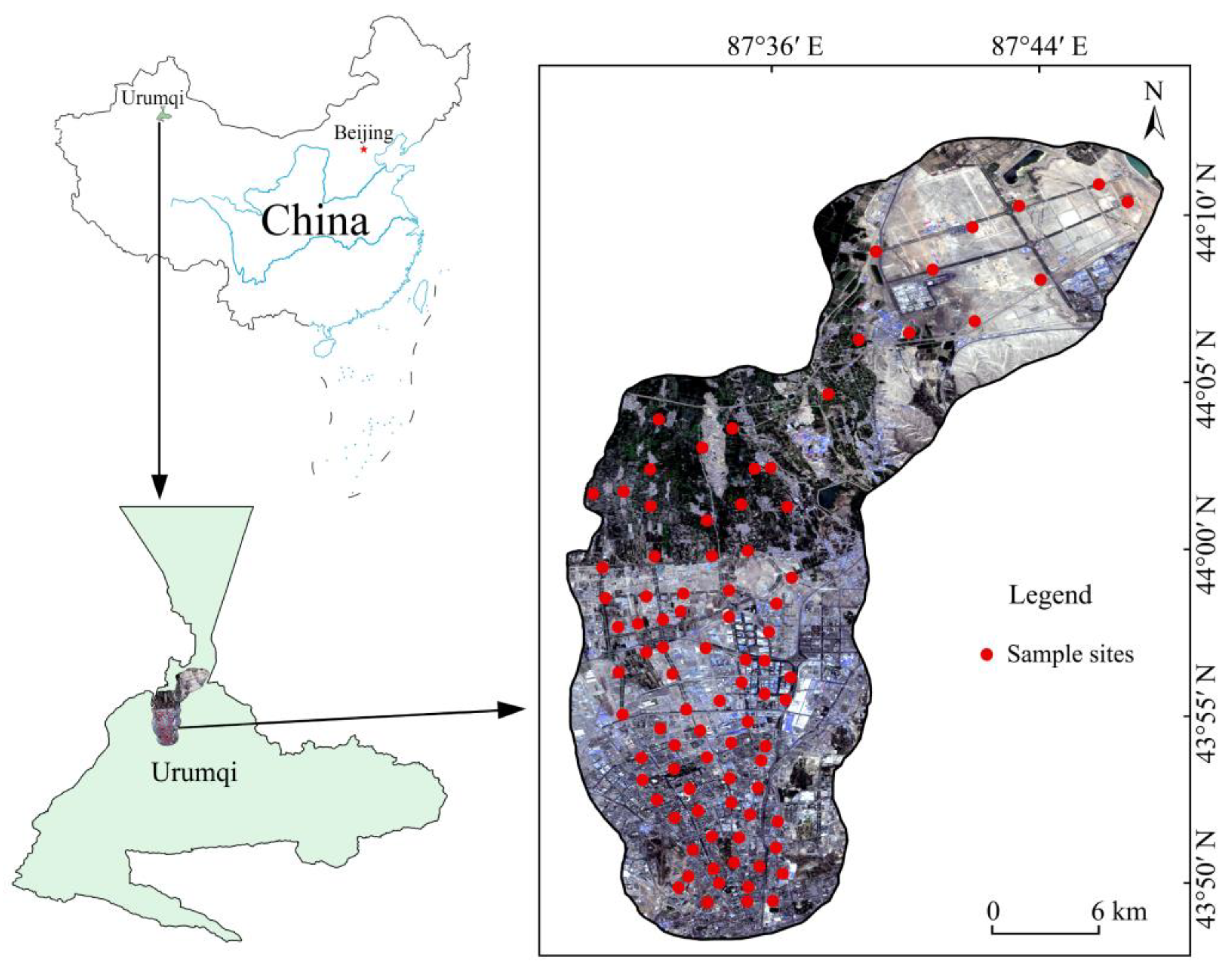
2. Description of the Study Area

The experimental field (87°28′–87°37′ E and 43°48′–44°04′ N) was selected in the central parts of the Urumqi, which is the capital of Xinjiang and the core city on the Silk Road Economic Belt. It is situated in the southern edge of the Junggar Basin, the northwest arid regions of China, and is one of the important metropolitan cities in NW China (Figure 1). The main soil type is mainly grey desert soil [29], and the climate of the study area is regionally marked by a continental arid climate. The annual average temperature, precipitation, and evaporation are about 6.7 °C, 280 mm, and 2730 mm, respectively. In recent years, the accelerated process of urbanization, expanding scale of industrial and agricultural production, and the increase in emissions from production and living have led to the Ni contamination of the soil in the study area [29,30].

3. Experimental Data

3.1. Sample Collection and Analysis

A total of 88 topsoil samples were collected from the study area in April of 2021, as illustrated in Figure 1. At each of the sample sites, five sub-samples were taken from the topsoil layer (0–20 cm) within 100 m × 100 m areas, and then mixed together to form a composite soil sample, weighing more than 500 g. All the soil samples were returned to the laboratory and sieved through 20 meshes after they were naturally air dried. Each sample was divided into two groups: one for the determination of the Ni content and another for the hyperspectral measurement. The soil Ni content was determined, as described in “HJ 803–2016” [31], using an Inductively Coupled Plasma Mass Spectrometer (ICP–MS 7800). All the soil samples were tested repeatedly, and the determined consistency of the Ni measurements was 95.6%.

3.2. Spectrometric Determination

The spectral determination of the collected soil samples was measured using a FieldSpec®3 (ASD, Boulder, CO, USA) portable object spectrometer manufactured by Analytical Spectral Devices. The interval of data acquisition was 1 nm, with a spectral measurement range from 350 to 2500 nm. Firstly, the instrument was preheated, and secondly, a 40 cm × 40 cm white board was placed on a 2 m × 2 m black cardboard for calibration to obtain the absolute reflectance before determining the spectral data. Finally, the soil samples were kept in a natural state on the black cardboard with the sensor probe perpendicular to 15 cm above the soil surface, and the sensor probe was optimized with a white board every 5 min. A total of 15 replicate measurements were taken on the same soil sample, and 15 spectral curves were collected.

4. Experimental Data

4.1. Spectral Analysis

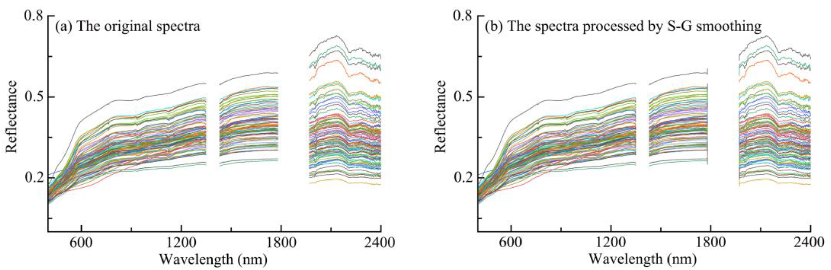
4.1.1. Spectral Data Pre-Processing

A total of 15 spectral curves were measured for each soil sample, and the 15 spectral curves were averaged using ViewSpecPro (Version 5.6) software, and the arithmetic mean was taken as the original reflectance spectral value of the soil sample. Due to the influence of the surrounding environment and the spectral instrument itself, the spectral bands within 350–399 nm, 1350–1430 nm, 1781–1970 nm, and 2401–2500 nm were excluded before constructing the hyperspectral models, which was outputted in a total of 1730 bands.
Finally, the original spectra of soil samples were smoothed using the Savitzky–Golay (S–G) method. The S–G filter algorithm is a weighted filtering of the data, which has the advantage of retaining the information about the variation of the signal more effectively, removing noise from the spectral curves, and improving the smoothness of the spectrum during filter smoothing. Figure 2 illustrates the spectral reflectance curves of the original spectra and the spectra processed by the S–G smoothing.

4.1.2. Spectral Transformation

The original spectral response signals of the Ni in the soil are weak and it is difficult to directly reflect the important wavelengths with the original spectra data [32]. In order to enhance the spectral information related to the Ni in the soil samples, the original spectral reflectance data (R) were subjected to first-order differentiation (FD), second-order differentiation (SD), first-order differentiation of the reciprocal (RTFD), second-order differentiation of the reciprocal (RTSD), first-order differentiation of the logarithm (LTFD), second-order differentiation of the logarithm (LTSD), root mean square first-order differentiation (RMSFD), root mean square second-order differentiation (RMSSD), logarithmic first order differentiation of the reciprocal (ATFD), logarithmic second order differentiation of the reciprocal (ATSD), logarithmic first order differentiation of the reciprocal (RLFD), and logarithmic second order differentiation of the reciprocal (RLSD) equations.

4.1.3. Important Wavelengths Selection

Firstly, Pearson’s correlation coefficient analysis (PCC) was performed between the soil Ni content and 13 forms of the soil spectral data, and the bands with larger correlation coefficients were screened out as important wavelengths for hyperspectral prediction modeling.
Secondly, important wavelengths from all the original and 12 types of transformed spectral data were intelligently extracted using Competitive Adaptive Re-weighted Sampling (CARS), excluding further removed wavelengths with low correlation [33,34].

4.2. Modelling of Hyperspectral Inversion

In order to consider both the Ni content vector and the spectral vector, soil samples were randomly split into a modeling dataset (70 samples) and a validation dataset (18 samples). The modeling dataset was used to build hyperspectral prediction models, while the validation dataset was used to test the accuracy of the prediction models. The partial least squares regression (PLSR), random forest regression (RFR) and support vector machine regression (SVMR) models were used to select the optimum hyperspectral prediction model.
The PLSR algorithm can consider both the spectral information (x) and the corresponding reference values (y) of the samples during modeling and transform the original spectral data into mutually orthogonal and unrelated new variables via linear transformation, thereby eliminating multicollinearity between datasets [35].
The RFR technique is a new data mining technique which is designed to produce accurate predictions that do not overfit the data. Based on a bootstrapped training sample, the individual trees in the RFR ensemble are built, and only a small fraction of the predictor variables are considered in each segmentation; this ensures that trees are decorrelated with each other [36]. The RFR technique is easy to run because it requires only three input parameters: the number of two ‘random_state’ and ‘n_estimators’. The three input parameters are used to partition the modeling set and validation set and to determine the optimal partitioning of each tree node. Additionally, studies have shown that the three input parameters provide accurate results [32].
The SVMR model is a non-linear predictive model based on the kernel-based machine learning approach. It can use a specific transfer kernel function to map the spectrum matrix into a high-dimensional feature space and establish a hyperplane as a decision surface to segment different samples with the principle of interval-maximizing segmentation, and then in turn provides an inverse prediction of the heavy metal content of soil [37].

4.3. Model Validation

The determination coefficient (R2), root mean square error (RMSE), mean absolute error (MAE), and residual prediction deviation (RPD) are used to evaluate the prediction accuracy of the hyperspectral prediction models. A robust model has a higher R2 and RPD and a lower RMSE and MAE [38]. When R2 < 0.5, the prediction model does not have a predictive ability; when 0.5 ≤ R2 < 0.7, the model has a preliminary predictive capability; and when R2 ≥ 0.7, the model has a good predictive capability [39]. When RPD ≥ 2.0, the model has a better predictive ability; when 1.4 ≤ RPD < 2.0, the model has an initial predictive capability; and when RPD < 1.4, the model has a bad predictive capability. In general, a lower RMSE and MAE indicate better model prediction accuracy [40].

5. Results

5.1. Statistical Analysis of Ni Content in Soil

The statistical results of the Ni content of the soil samples in Urumqi are given in Table 1. Standard deviation (SD) and coefficient of variation (CV) analyses were used to measure data dispersion, where the CV complements the SD. Table 1 showed that the Ni content in the soil samples was distributed in the range of 10.00–29.00 mg/kg, and the average value was 18.52 mg/kg. The average Ni content of the modeling set and validation set were 18.71 mg/kg and 17.78 mg/kg, respectively. The SD of the modeling set and validation set were 3.59 and 2.92 mg/kg, respectively. Further, the CV values of the modeling set and validation set were 0.19 and 0.16, respectively. It is clear that the average, SD, and CV values of the Ni content in the modeling set were essentially the same as those of the validation set. This indicates that the division of soil samples was reasonable and can be used for subsequent model construction.

5.2. Correlation between Ni Content and Reflectance Data of Soil

The PCC analysis was performed between the Ni content and 13 forms of soil spectral data, which can identify the correlation between the Ni content and spectral data of soil samples. The degree of correlation was expressed by the Pearson coefficient (R), and Pearson’s correlation analysis was used in the significance test at the P < 0.01 level (two-sided).
In Figure 3, the original spectral data showed a weak correlation with the Ni content, with nine important wavelengths selected. The correlation analysis of the Ni content and spectral data processed by differential transformations indicated that both positive and negative correlation coefficients had extreme values, and the positive and negative correlations of the filtered important wavelengths were more uniformly distributed. Thus, both the original spectrum and all the transformed spectra can filter out characteristic bands for data modeling, and the number of the important wavelengths descended in the order of: RTFD(617) > LTFD(580) = ATFD(580) > RMSFD(499) > FD(426) > RTSD(355) > LTSD(289) = ATSD(289) > RLFD(279) > RMSSD(259) > SD(219) > RLSD(129) > R(9).
The number of important wavelengths selected by CARS descended in the following order: ATFD (26) > RTFD (25) = LTSD (25) > FD (24) > LTFD (23) >RLSD (22) = SD (22) > RTSD (21) = RMSSD (21) > ATSD (20) = RLFD (20) > RMSFD (17) > R (17). It can be shown that the number of important wavelengths was less than the Pearson’s correlation coefficient analysis expected for the original spectrum.

5.3. Establishment and Analysis of Hyperspectral Prediction Model

Partial least squares regression model (PLSR), random forest regression model (RFR), and support vector machine regression model (SVMR) were constructed for predicting the Ni content of soil in this study. Based on Python, a validation set was modeled, and the “random_state” of the three models was set as two. Due to the randomness of the RFR model, the number of parameters (“n_estimators” and another “random_state”) will disturb the predictive performance of the model. Under the consideration of model performance, model running time, sample number and other factors, the number of parameters (“n_estimators” and another “random_state”) of the RFR model was set in the range from one to ninety-nine. In order to consider both the soil Ni content vector and the spectral vector, the soil samples were split into a modeling set and validation set for modeling and verification, respectively. The number of modeling sets and validation sets were 70 and 18, respectively. According to the correlation coefficient between the Ni content and spectrum data, wavelengths with absolute values of more than 0.272 under the processed spectral reflectance data were taken as important wavelengths. Then, important wavelengths were selected as the independent variables (x), and the Ni content of the soil was selected as the dependent variable (y). The hyperspectral prediction model for the Ni content was established by the partial least squares regression (PLSR), the random forest regression (RFR), and support vector machine regression (SVMR) algorithms, respectively.

5.3.1. The Analysis of PLSR Model

The basic statistics related to the stability and accuracy of the PLSR model is given in Table 2. The R2, inversed by the PLSR model based on the important wavelengths selected by PCC, ranged from 0.012 to 0.603; RMSE values ranged from 1.838 to 3.032; MAE values ranged from 1.248 to 1.520; and RPD values ranged from 0.963 to 1.589. The accuracy of the PLSR model based on the original spectrum (R), was lower than the model based on the 12 transformations (RMSFD, RMSSD, LTFD, LTSD, RLFD, RLSD, RTFD, RTSD, ATFD, ATSD, FD, SD). The FD-PLSR model had the best predictive capability (R2 = 0.603, RMSE = 1.838, MAE = 1.249, RPD = 1.589). The ranges of the R2, RMSE, MAE, and RPD values inversed by the PLSR model based on the important wavelengths selected by CARS, were 0.388–0.736, 1.498–2.282, 1.309–1.144, and 1.280–1.949, respectively. The predictive accuracy of the PLSR model has been improved to different degrees with 10 transformations (RMSFD, RMSSD, LTFD, RLFD, RLSD, RTFD, RTSD, ATFD, ATSD, SD) processed by CARS. The prediction accuracy of the CARS-RMSFD-PLSR model was the highest (R2 = 0.736, RMSE = 1.498, MAE = 1.144, RPD = 1.949). In general, CARS is superior to PCC, and the CARS-RMSFD-PLSR model is better than the FD-PLSR model.
A map of the spatial distribution (Figure 4) illustrates the relationship between the measured and CARS-RMSFD-PLSR predicted content of Ni in the soil in the study area. The results indicated that the accuracy of the PLSR estimation model was not high.

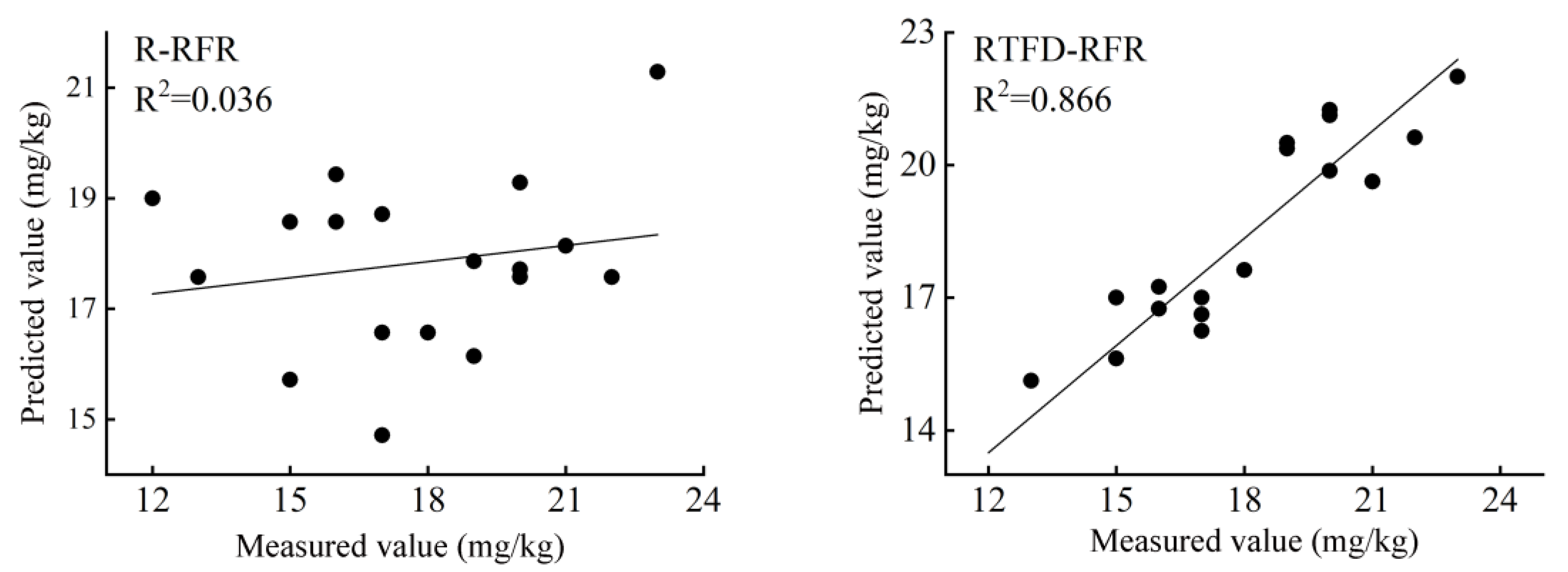
5.3.2. The Analysis of RFR Model

In Table 3, the ranges of the R2, RMSE, MAE, and RPD values, inversed by the RFR model based on the important wavelengths selected by the PCC, were 0.036–0.866, 1.321–9.096, 0.986–2.563, and 0.321–2.210, respectively. The R2 was higher than 0.5 except for R, so RFR model has good predictive ability. The accuracy of the RFR model based on the transformed spectrum was higher than the original spectrum (R). The best inverse prediction model was the RTFD-RFR model (R2 = 0.866, RMSE = 1.321, MAE = 0.986, RPD = 2.210). The R2, inversed by the RFR model based on the important wavelengths selected by CARS, ranged from 0.408 to 0.837; the ranges of the RMSE and MAE values were 1.388–5.037 and 0.958–1.910; and the RPD values were 0.580–2.104. Except for three transformations (RLSD, ATSD, SD), the prediction accuracy of the model based on the remaining nine transformations by CARS, declined to different degrees.
The prediction accuracy of the CARS-ATSD-RFR model was the highest (R2 = 0.837, RMSE = 1.388, MAE = 0.958, RPD = 2.104). The PCC was superior to CARS, and the RTFD-RFR model was better than the CARS-ATSD-RFR model.
A map of the spatial distribution (Figure 5) illustrates the relationship between the measured and RTFD-RFR predicted content of Ni in the soil in the study area. As shown in Figure 5, the estimated Ni (Figure 5B) content, based on the RTFD-RFR method, showed very similar distribution patterns as the laboratory-measured Ni content (Figure 5A). The results illustrated in Figure 5 further explain that the estimation model based on the RTFD-RFR has a high degree of accuracy for estimating the Ni content in urban soil.

5.3.3. The Analysis of SVMR Model

The basic statistics related to the stability and accuracy of the SVMR model is given in Table 4. The R2, inversed by the SVMR model based on the important wavelengths selected by PCC, ranged from 0.071 to 0.648; the values of the RMSE and MAE ranged from 1.730 to 2.963 and from 1.408 to 2.415, respectively; the RPD values ranged from 1.688 to 0.985. The accuracy of the SVMR model based on the original spectrum (R) was lower than the model based on 12 transformations (RMSFD, RMSSD, LTFD, LTSD, RLFD, RLSD, RTFD, RTSD, ATFD, ATSD, FD, SD). The ATSD-SVMR model has the best predictive capability (R2 = 0.648, RMSE = 1.730, MAE = 1.408, RPD = 1.688). The ranges of the R2, RMSE, MAE, and RPD values, inversed by the SVMR model based on the important wavelengths selected by CARS, were 0.106–0.630, 1.774–2.757, 1.353–2.120, and 1.059–1.646, respectively.
The prediction accuracy of the CARS-RLSD-SVMR model was the highest (R2 = 0.630, RMSE = 1.774, MAE = 1.353, RPD = 1.646). PCC was better than CARS, and the ATFD-PLSR model was better than CARS-RLSD-SVMR model.
A map of the spatial distribution (Figure 6) illustrates the relationship between the predicted and measured content of Ni in the soil in the study area.
As shown in Figure 5, the predictive accuracy of the SVMR estimation model was not high.

5.4. Discussion of Optimal Prediction Models

The hyperspectral inversion of soil Ni content is influenced by two aspects; on the one hand, estimating Ni content in soil using hyperspectral remote sensing is a cost-efficient method, but challenging due to the effects of natural environmental conditions and soil properties [41]. On the other hand, high-data dimensionality is a common problem in hyperspectral data processing [32], so the inversion accuracy of the constructed model is biased by redundant spectra and noise [42]. Wang et al. [40] have pointed out that spectral transformation is an effective approach for identifying the highly correlated spectral bands. Yuan et al. [33] believed that using the CARS method can effectively eliminate redundant information, greatly improve the correlation, and increase the efficiency. Chen et al. [43] have constructed a model, based on the random forest regression technique, that can effectively predict the soil Ni content in Taiwan Province, China (R2 = 0.63, RMSE = 150.02, MAPE = 31.93). Zhang et al. [44] have pointed out that the CWT-RBF hyperspectral inversion model (R2 = 0.88, RMSE = 2.41, RPD = 3.91) is a great method to predict the soil Ni content in Gulin County, Sichuan Province, China. Hou et al. [14] have analyzed and concluded that the PLSR model (R2 = 0.879, RMSE = 1.292) is an ideal model for predicting the soil Ni content of Zoucheng, Shandong Province, China. Yang et al. [45] have found that the partial least squares regression model has the highest predictive ability for the inversion of soil Ni content in the Shizishan mining area in Tongling city, Anhui Province.
In this study, the inversion accuracy of the Ni content in soil can be ranked as follows: R2RTFD-RFR > R2CARS-ATSD-RFR > R2CARS-RMSFD-PLSR > R2ATSD-SVMR > R2CARS-RLSD-SVMR > R2FD-PLSR. Therefore, combined with the performance of the inversion accuracy of the Ni content in soil, the inversion accuracy of the RFR method is significantly better than that of the PLSR and SVMR methods. As shown in Table 2, Table 3 and Table 4, the fitness, stability, and accuracy of the inversion model are changed in different degrees by the processing methods of the original spectral data (R). The best inverse prediction model is the RTFD-RFR model (R2 = 0.866, RMSE = 1.321, MAE = 0.986, RPD = 2.210), which has a better ability to invert the soil heavy metal content in the study area. The scatter plot of Ni content modeling by the RTFD-RFR and R-RFR model is exhibited in Figure 7.
The R2 calculated by the RFR model based on the RTFD transformation of the important spectral wavelengths is significantly higher than that modelled from the original spectral data (R), and both the RMSE and MAE are significantly decreased. From Figure 7, the accuracy of the RFR model based on R was not high, and the R2 was 0.036. The modelling prediction accuracy of the RTFD transformation was improved significantly, and the predicted and measured values presented strong agreement with each other, with an R2 of 0.866, which was improved by 0.830 compared with the R-RFR model. The measured values of the Ni content of the soil samples in this study had a small range of fluctuation and no extreme points, but whether they were modelled with the original spectrum or with the transformed important spectral wavelengths, the predicted values were slightly higher when the measured values were low, and slightly lower when the measured values were high, which suggests that the inaccuracy may have come from the extreme points; however, due to the limited number of sample points in this study, there were no extreme sample points, which was a limitation of the study.
Overall, a faster and convenient method for estimating the Ni content in soil was described in this work. This method provides an effective way for predicting the Ni content in urban soil. The results obtained in this study are in agreement with the results of previous studies [11,38,39,40], which implies that the Ni content of soil can be assessed using hyperspectral remote sensing technology with reasonable accuracy. The results of this study support the use of a remote sensing technical approach for characterizing the Ni content in urban soil.

6. Conclusions

To find an optimal inversion model to predict soil Ni content, hyperspectral prediction models were constructed based on the important wavelengths and Ni content from field soil samples. The results of this study lead to the following conclusions:
  • Transformed spectral data with Pearson’s correlation coefficient analysis and the CARS method can obviously reduce the interference of the environmental background and improve the correlations between spectral reflectance data and the Ni content of soil. However, the spectral reflectance data correlate differently with the Ni content under different spectral processing methods. The first-order differentiation of the reciprocal (RTFD) has the most significant enhancement of spectral features.
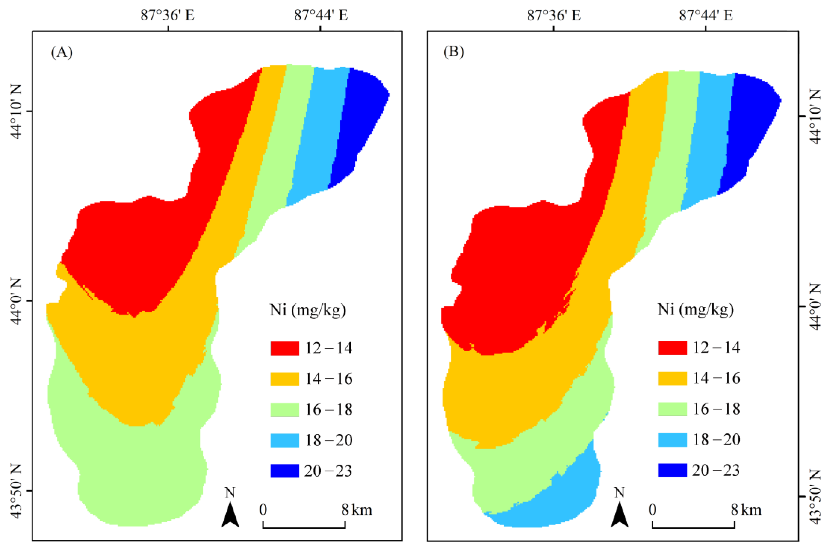
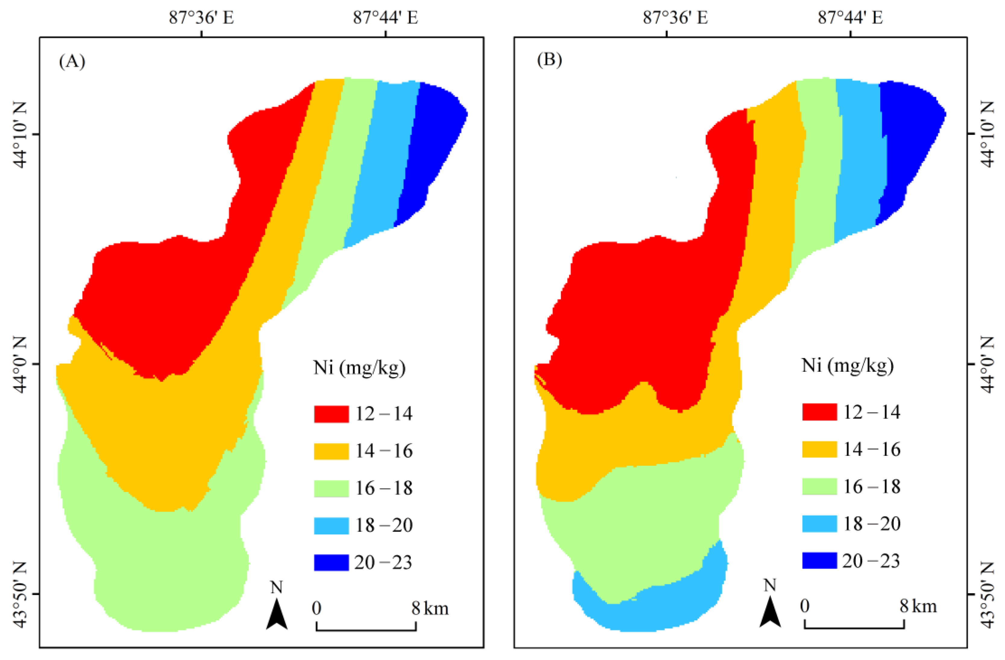
  • The results showed that the RTFD–RFR model is more stable and has the best inversion effects, with the highest predictive ability (R2 = 0.866, RMSE = 1.321, MAE = 0.986, RPD = 2.210) for determining the Ni content in soil in the research region. The RTFD–RFR model can be used as a means of predicting the Ni content in urban soil.
Overall, the results of this study demonstrate the possibility of directly applying hyperspectral remote sensing approaches to estimating Ni content in urban soil. This method can provide a technical support for the hyperspectral inversion and rapid detection of soil Ni content. However, this study lacks the combination of hyperspectral and remote sensing imagery, which needs to be further verified in subsequent studies.

Author Contributions

Q.Z. completed all the experiments to obtain data, processed the data, and wrote the main manuscript text. M.E. provided the support and gave guidance for this study. R.S. and M.A. taught the methods. Q.Z., M.E., R.S., M.A., H.L. and L.W. reviewed the manuscript. All authors have read and agreed to the published version of the manuscript.

Funding

This research is funded by the National Natural Science Foundation of China (grant number U2003301), and the Tianshan Talent Training Project of Xinjiang.

Institutional Review Board Statement

Not applicable.

Informed Consent Statement

Not applicable.

Data Availability Statement

Data will be available upon request to the corresponding author.

Conflicts of Interest

The authors declare no conflict of interest.

References

  1. World Health Organization. International Agency for Research on Cancer Group II Carcinogen List; World Health Organization: Geneva, Switzerland, 2017. [Google Scholar]
  2. Chen, M.Y.; Zhu, H.H.; She, W.D.; Yin, G.C.; Huang, Z.Z.; Yang, Q.L. Health risk assessment and source apportionment of soil heavy metals at a legacy shipyard site in Pearl River Delta. Ecol. Environ. Sci. 2023, 32, 794–804. [Google Scholar]
  3. Ning, W.J.; Xie, X.M.; Yan, L.P. Spatial distribution, sources and health risks of heavy metals in soil in Qingcheng District, Qingyuan City: Comparison of PCA and PMF model results. Earth Sci. Front. 2023, 30, 470–484. [Google Scholar]
  4. Guo, Z.J.; Zhou, Y.L.; Wang, Q.L. Characteristics of soil heavy metal pollution and health risk in Xiong’an New District. China Environ. Sci. 2021, 41, 431–441. [Google Scholar]
  5. Ajigul, M.; Mamattursun, E.; Anwar, M. Pollution risk assessment of heavy metals from farmland soils in urban-rural ecotone of Kashgar City, XinJiang. Environ. Eng. 2018, 36, 160–164. [Google Scholar]
  6. Li, J.; Li, X.; Li, K.M.; Jiao, L.; Tai, X.S.; Zang, F. Characteristics and identification priority source of heavy metals pollution in farmland soils in the Yellow River Basin. Environ. Sci. 2023, 44, 4406–4415. [Google Scholar] [CrossRef]
  7. Ali, R.; Hossein, H.; Seyedeh, B.F.M.; Nima, J. Evaluation of heavy metals concentration in Jajarm Bauxite Deposit in northeast of Iran using environmental pollution indices. Malays. J. Geosci. 2019, 12, 12–20. [Google Scholar]
  8. Ali, R.; Hossein, H.; Seyedeh, B.F.M.; Sara, H.; Nima, J. Assessment of heavy metals contamination in surface soils in Meiduk copper mine area, Se Iran. Earth Sci. Malays. 2019, 3, 1–8. [Google Scholar]
  9. Xue, Y.; Zou, B.; Wen, Y.; Tu, Y.; Xiong, L. Hyperspectral inversion of chromium content in soil using support vector machine combined with lab and field spectra. Sustainability 2020, 12, 4441. [Google Scholar] [CrossRef]
  10. Patel, A.K.; Ghosh, J.K.; Sayyad, S.U. Fractional abundances study of macronutrients in soil using hyperspectral remote sensing. Geocarto Int. 2020, 37, 474–493. [Google Scholar] [CrossRef]
  11. Yang, Y.; Cui, Q.; Jia, P.; Liu, J.; Bai, H. Estimating the heavy metal concentrations in topsoil in the Daxigou mining area, China, using multispectral satellite imagery. Sci. Rep. 2021, 11, 11718. [Google Scholar] [CrossRef]
  12. Ye, M.; Zhu, L.; Li, X.; Ke, Y.; Huang, Y.; Chen, B.; Yu, H.; Li, H.; Feng, H. Estimation of the soil arsenic concentration using a geographically weighted XGBoost model based on hyperspectral data. Sci. Total. Environ. 2022, 858, 159798. [Google Scholar] [CrossRef]
  13. Hou, L.; Li, X.; Li, F. Hyperspectral-based inversion of heavy metal content in the soil of coal mining areas. J. Environ. Qual. 2018, 48, 57–63. [Google Scholar] [CrossRef]
  14. Surya, S.G.; Yuvaraja, S.; Varrla, E.; Baghini, M.S.; Palaparthy, V.S.; Salama, K.N. An in-field integrated capacitive sensor for rapid detection and quantification of soil moisture. Sens. Actuators B Chem. 2020, 321, 128542. [Google Scholar] [CrossRef]
  15. Samuel, N.A.; Anna, F.H.; Andreas, A.; Joshua, H.V.; Teamrat, A.G. Advances in soil moisture retrieval from multispectral remote sensing using unoccupied aircraft systems and machine learning techniques. Hydrol. Earth Syst. Sci. 2021, 25, 2739–2758. [Google Scholar]
  16. Asmau, M.A.; Olga, D.; Yahya, Z.; Mike, S. Quantification of hydrocarbon abundance in soils using deep learning with dropout and hyperspectral data. Remote Sens. 2019, 11, 1938. [Google Scholar]
  17. Li, H.; Jia, S.; Le, Z. Quantitative Analysis of soil total nitrogen using hyperspectral imaging technology with extreme learning machine. Sensors 2019, 19, 4355. [Google Scholar] [CrossRef] [PubMed]
  18. Xu, X.; Chen, S.; Xu, Z.; Yu, Y.; Zhang, S.; Dai, R. Exploring appropriate preprocessing techniques for hyperspectral soil organic matter content estimation in black soil area. Remote Sens. 2020, 12, 3765. [Google Scholar] [CrossRef]
  19. Jia, P.; Zhang, J.; He, W.; Hu, Y.; Zeng, R.; Zamanian, K.; Jia, K.; Zhao, X. Combination of hyperspectral and machine learning to invert soil electrical conductivity. Remote Sens. 2022, 14, 2602. [Google Scholar] [CrossRef]
  20. Avdan, U.; Kaplan, G.; Matcı, D.K.; Avdan, Z.Y.; Erdem, F.; Mızık, E.T.; Demirtaş, I.K. Soil salinity prediction models constructed by different remote sensors. Phys. Chem. Earth Parts A/B/C 2022, 128, 103230. [Google Scholar] [CrossRef]
  21. Jia, P.; Zhang, J.; He, W.; Yuan, D.; Hu, Y.; Zamanian, K.; Jia, K.; Zhao, X. Inversion of different cultivated soil types’ salinity using hyperspectral data and machine learning. Remote Sens. 2022, 14, 5639. [Google Scholar] [CrossRef]
  22. Wei, L.; Pu, H.; Wang, Z.; Yuan, Z.; Yan, X.; Cao, L. Estimation of soil arsenic content with hyperspectral remote sensing. Sensors 2020, 20, 4056. [Google Scholar] [CrossRef] [PubMed]
  23. Tan, K.; Ma, W.; Chen, L.; Wang, H.; Du, Q.; Du, P.; Yan, B.; Liu, R.; Li, H. Estimating the distribution trend of soil heavy metals in mining area from HyMap airborne hyperspectral imagery based on ensemble learning. J. Hazard. Mater. 2021, 401, 123288. [Google Scholar] [CrossRef] [PubMed]
  24. Xia, F.; Peng, J.; Wang, Q.L.; Zhou, L.Q.; Shi, Z. Prediction of heavy metal content in soil of cultivated land: Hyperspectral technology at provincial scale. J. Infrared Millim. Waves 2015, 34, 594–600. [Google Scholar]
  25. Zhao, Y.L.; Yang, N.N.; Zhang, H.X.; Wang, X.J.; Sun, X.Y.; Wang, W. Study on the statistical estimation model of soil heavy metals in Handan city based on hyper-spectral. Ecol. Environ. Sci. 2020, 29, 819–826. [Google Scholar]
  26. Guo, X.F.; Cao, Y.; Jiao, R.C.; Nan, Y.; Zhao, Y.F.; Ding, X. An inversion of soil nickel contents with hyperspectral in iron mine area of Beijing. Chin. J. Soil Sci. 2021, 52, 960–967. [Google Scholar]
  27. Wang, F.H.; Lu, J.H.; Liu, Z.W.; Wang, D.Q.; Li, X.C. Estimation of soil heavy metal nickel in Yantai District based on hyperspectral data. J. Shandong Agric. Univ. (Nat. Sci. Ed.) 2019, 50, 84–87. [Google Scholar]
  28. Ni, B.; Huang, Z.Q.; Jiang, M.; Zhang, Y.L.; Zhu, F.X. Retrieval of heavy metal nickel content in farmland soil in the southwest of Xiong’an New District based on aerial hyperspectral CASI & SASI data. Geol. Explor. 2022, 58, 1307–1320. [Google Scholar]
  29. Nazupar, S.; Mamattursun, E.; Li, X.; Wang, Y. Spatial distribution, contamination levels, and health risks of trace elements in topsoil along an urbanization gradient in the city of Urumqi, China. Sustainability 2022, 14, 12646–12663. [Google Scholar]
  30. Wei, B.; Jiang, F.; Li, X.; Mu, S. Spatial distribution and contamination assessment of heavy metals in urban road dust from Urumqi, NW China. Microchem. J. 2002, 93, 147–152. [Google Scholar] [CrossRef]
  31. CMEPRC (Ministry of Environmental Protection of the People’s Republic of China). Soil and Sediment—Determination of Aqua Regia Extracts of 12 Metal Elements—Inductively Coupled Plasma Mass Spectrometry, HJ 803–2016. 2016. Available online: https://www.doc88.com/p-3357828192459.html (accessed on 15 January 2019).
  32. Michelle, D.; Onisimo, M.; Riyad, I. Examining the utility of random forest and AISA Eagle hyperspectral image data to predict Pinus patula age in KwaZulu-Natal, South Africa. Geocarto Int. 2011, 26, 275–289. [Google Scholar]
  33. Yuan, Z.R.; Wei, L.F.; Zhang, Y.X.; Yu, M.; Yan, X.R. Hyperspectral inversion and analysis of heavy metal arsenic content in farmland soil based on optimizing CARS combined with PSO-SVM algorithm. Spectrosc. Spectr. Anal. 2020, 40, 567–573. [Google Scholar]
  34. Zhong, X.J.; Yang, L.; Zhang, D.X.; Cui, T.; He, X.T.; Du, Z.H. Effect of different particle sizes on the prediction of soil organic matter content by visible-near infrared spectroscopy. Spectrosc. Spectr. Anal. 2022, 42, 2542–2550. [Google Scholar]
  35. Ma, X.; Zhou, K.; Wang, J.; Cui, S.; Zhou, S.; Wang, S.; Zhang, G. Optimal bandwidth selection for retrieving Cu content in rock based on hyperspectral remote sensing. J. Arid. Land 2022, 14, 102–114. [Google Scholar] [CrossRef]
  36. Breiman, L. Random Forest. Mach. Learn 2001, 45, 5–32. [Google Scholar] [CrossRef]
  37. Han, L.; Chen, R.; Zhu, H.; Zhao, Y.; Liu, Z.; Huo, H. Estimating soil arsenic content with visible and near-infrared hyperspectral reflectance. Sustainability 2020, 12, 1476. [Google Scholar] [CrossRef]
  38. Rukeya, S.; Nijat, K.; Abdugheni, A.; Li, H.; Ahunaji, Y.; Balati, M.; Shi, Q.D. Possibility of optimized indices for the assessment of heavy metal contents in soil around an open pit coal mine area. Int. J. Appl. Earth Obs. Geoinf. 2018, 73, 14–25. [Google Scholar]
  39. Vohland, M.; Besold, J.; Hill, J.; Fründ, H.-C. Comparing different multivariate calibration methods for the determination of soil organic carbon pools with visible to near infrared spectroscopy. Geoderma 2011, 166, 198–205. [Google Scholar] [CrossRef]
  40. Wang, Y.; Niu, R.; Lin, G.; Xiao, Y.; Ma, H.; Zhao, L. Estimate of soil heavy metal in a mining region using PCC-SVM-RFECV-AdaBoost combined with reflectance spectroscopy. Environ. Geochem. Health 2023. online ahead of print. [Google Scholar] [CrossRef]
  41. Liu, W.; Li, M.; Zhang, M.; Long, S.; Guo, Z.; Wang, H.; Li, W.; Wang, D.; Hu, Y.; Wei, Y.; et al. Hyperspectral inversion of mercury in reed leaves under different levels of soil mercury contamination. Environ. Sci. Pollut. Res. 2020, 27, 22935–22945. [Google Scholar] [CrossRef]
  42. Zhou, M.; Zou, B.; Tu, Y.; Feng, H.; He, C.; Ma, X.; Ning, J. Spectral response feature bands extracted from near standard soil samples for estimating soil Pb in a mining area. Geocarto Int. 2022, 37, 13248–13267. [Google Scholar] [CrossRef]
  43. Chen, H.W.; Chen, C.-Y.; Nguyen, K.L.P.; Chen, B.-J.; Tsai, C.-H. Hyperspectral sensing of heavy metals in soil by integrating AI and UAV technology. Environ. Monit. Assess. 2022, 194, 518. [Google Scholar] [CrossRef] [PubMed]
  44. Zhang, S.; Shen, Q.; Nie, C.; Huang, Y.; Wang, J.; Hu, Q.; Ding, X.; Zhou, Y.; Chen, Y. Hyperspectral inversion of heavy metal content in reclaimed soil from a mining wasteland based on different spectral transformation and modeling methods. Spectrochim. Acta Part A Mol. Biomol. Spectrosc. 2019, 211, 393–400. [Google Scholar] [CrossRef] [PubMed]
  45. Yang, H.; Xu, H.; Zhong, X. Study on the hyperspectral retrieval and ecological risk assessment of soil Cr, Ni, Zn heavy metals in tailings area. Bull. Environ. Contam. Toxicol. 2022, 108, 745–755. [Google Scholar] [CrossRef] [PubMed]
Figure 1. Location of experimental field and sample sites.
Sustainability 15 13948 g001
Figure 2. The spectral reflectance curves of soil of the original spectra (a) and the spectra processed by the Savitzky–Golay smoothing (b).
Sustainability 15 13948 g002
Figure 3. Correlations between soil Ni content and spectral reflectance data.
Sustainability 15 13948 g003
Figure 4. Comparison of Ni distribution maps of field measured values (A) and predicted values by PLSR (B).
Sustainability 15 13948 g004
Figure 5. Comparison of Ni distribution maps of field measured values (A) and predicted values by RFR (B).
Sustainability 15 13948 g005
Figure 6. Comparison of Ni distribution contour maps of field measured values (A) and predicted values by SVMR (B).
Sustainability 15 13948 g006
Figure 7. Measured and RTFD-RFR predicted values of Ni content in soil.
Sustainability 15 13948 g007
Table 1. Statistical values of Ni content in soil in Urumqi.
Data SetSamples/nMinimumMaximumAverageSDCV
Modeling set (mg/kg)7010.0029.0018.713.590.19
Validation set (mg/kg)1812.0023.0017.782.920.16
Total (mg/kg)8810.0029.0018.523.490.19
Table 2. Statistics of accuracy parameters of PLSR model for soil Ni content in Urumqi.
TransformationPCCCARS
R2RMSEMAERPDR2RMSEMAERPD
R0.0123.0321.5200.9630.4952.0731.3161.409
RMSFD0.5711.9101.2711.5290.7361.4981.1441.949
RMSSD0.3942.2711.3641.2860.6381.7561.1871.663
LTFD0.5142.0331.3001.4360.6151.8101.2281.613
LTSD0.4172.2261.3491.3120.4922.0791.2551.405
RLFD0.5671.9191.3001.5220.5371.9861.2871.470
RLSD0.4362.1911.3571.3330.5561.9421.2461.504
RTFD0.5851.8801.2481.5530.5451.9681.2781.484
RTSD0.4132.2351.3311.3060.6711.6731.1491.745
ATFD0.5152.0321.2991.4370.5661.9211.3091.520
ATSD0.4192.2241.3461.3130.6801.6511.1441.769
FD0.6031.8381.2491.5890.3882.2821.2881.280
SD0.3852.2871.3901.2770.6031.8371.1971.590
Table 3. Statistics of accuracy parameters of RFR model for Ni content of soils in Urumqi.
TransformationPCCCARS
R2RMSEMAERPDR2RMSEMAERPD
R0.0369.0962.5630.3210.7552.0831.2221.402
RMSFD0.7741.9241.0561.5180.4614.5871.7830.637
RMSSD0.8071.6441.0301.7760.7252.3411.1771.247
LTFD0.5823.5561.4670.8210.4085.0371.9100.580
LTSD0.7921.7671.0371.6530.7322.2811.1711.280
RLFD0.7622.0271.1671.4410.5463.8641.5610.756
RLSD0.7352.2531.2171.2960.7562.0771.1331.406
RTFD0.8661.3210.9862.2100.6842.6911.1981.085
RTSD0.6732.7841.2781.0490.7222.3641.2411.235
ATFD0.6223.2191.4140.9070.4254.8891.9790.597
ATSD0.7402.2121.1211.3200.8371.3880.9582.104
FD0.6492.9841.4720.9790.4534.6521.7010.628
SD0.7622.0201.0791.4460.7831.8501.0631.578
Table 4. Statistics of accuracy parameters of SVMR model for Ni content of soils in Urumqi.
TransformationPCCCARS
R2RMSEMAERPDR2RMSEMAERPD
R0.0712.9632.4150.9850.2422.5402.0851.150
RMSFD0.6211.7951.4761.6270.1062.7572.1201.059
RMSSD0.5941.8591.4641.5710.5741.9031.4681.534
LTFD0.5961.8531.4851.5760.1222.7332.2001.068
LTSD0.6111.8191.4251.6050.6121.8161.3591.608
RLFD0.6301.7741.4571.6460.1982.6122.0841.118
RLSD0.6271.7811.4051.6400.6301.7741.3531.646
RTFD0.4122.2371.7061.3050.2122.5891.9621.128
RTSD0.5761.8981.4951.5380.6111.8201.3951.604
ATFD0.5971.8501.4831.5780.1812.6402.0711.106
ATSD0.6481.7301.4081.6880.5931.8611.4371.569
FD0.6351.7611.4261.6580.3222.4021.8671.216
SD0.6051.8341.4251.5920.5042.0551.6051.421
Disclaimer/Publisher’s Note: The statements, opinions and data contained in all publications are solely those of the individual author(s) and contributor(s) and not of MDPI and/or the editor(s). MDPI and/or the editor(s) disclaim responsibility for any injury to people or property resulting from any ideas, methods, instructions or products referred to in the content.

