Enhancing the Dynamic Stability of Integrated Offshore Wind Farms and Photovoltaic Farms Using STATCOM with Intelligent Damping Controllers

Abstract

To build a large-scale renewable energy integrated system in the power system, power fluctuation mitigation and damping measures must be implemented during grid connection. PID damping controllers and traditional intelligent controllers with pole configuration are usually used for improving damping. Integration of large wind power plants and photovoltaic power plants into the power system faces transient power oscillation and fault ride-through (FRT) capability under fault conditions. Therefore, this paper proposes a static synchronous compensator (STATCOM) damper based on a recurrent Petri fuzzy probabilistic neural network (RPFPNN) to improve the transient stability of the power system when large offshore wind farms and photovoltaic power plants are integrated into the power system, suppress power fluctuation, and increase FRT capability. To verify the effectiveness of the proposed control scheme, a three-phase short circuit fault at the connected busbar is modeled in the time domain as part of a nonlinear model. From the comparison of simulation results, the proposed control scheme can effectively slow down the transient fluctuation of power supply to the grid-connected point when the grid is faulty, reach steady-state stability within 1–1.5 s, and reduce overshoot by more than 50%. It can also provide system voltage support at an 80% voltage drop and assist in stabilizing the system voltage to increase FRT capability. It also improves stability more than PID controllers when disturbances are present. Therefore, it maximizes the stability and safety of the power grid system.

1. Introduction

As a result of the continued improvement of economic conditions over the past few years, renewable energy has developed, particularly solar and wind energy [1]. Both of these sources of energy have resources in abundance, are widely distributed, and are known as “clean energy” in the industry [2]. Since natural resources are being consumed in such large quantities worldwide, countries are focusing on developing clean energy sources [3]. The characteristics of solar and wind energy make them among the most abundant sources of clean energy because they are pollution-free and durable [4].

Large-scale application of photovoltaic power generation technology is the forecasted development trend. The overvoltage phenomenon caused by solar panels connected to the power grid is theoretically analyzed in this paper. Additionally, the power control scheme of the grid is studied in combination with the characteristics of the grid lines [5]. PV power generation technology requires a reasonable control strategy to improve the voltage stability of the power system [6]. For comparisons of electricity grid performance after wind power integration, it is important to take into account the mutual influence between the power grid and wind farms. Most commonly, this influence is used to compare a wind farm’s installed capacity with the power grid’s strength, which is also a common method of analyzing offshore wind farms’ grid connections. When the grid voltage drops or surges, it will also affect the safe operation of offshore wind farms (OWF), which necessitates that OWFs have the ability to ride through failures. Offshore wind farms face high wind speeds and strong wind power [7]. Especially in the monsoon period, wind energy resources are extremely rich. A large amount of wind power is being generated at this time. The remote transmission of large-scale wind power sources often results in high line voltage drops [8]. Wind farms also absorb more reactive energy from the main network, resulting in insufficient reactive power, reducing the stability margin of the system, increasing the difficulty of node voltage regulation. Substations along a wind farm need to maintain a bus voltage of 1.1 times its rated voltage or more to support the normal system voltage. Insufficient voltage regulation capacity will also cause hidden dangers to the safe operation of power transmission and transformation equipment [9].

In practice, renewable energy consists of multiple types, and it is difficult to control the reactive power of all energy sources simultaneously in order to supply the system with enough reactive power [10]. To integrate renewable energy into the power system on a large scale, power fluctuation mitigation and damping improvement strategies during grid connection are crucial. When a catastrophic failure occurs, generation equipment loses synchronization and disconnects renewable energy from the grid. Thus, a VAR compensator is required to ensure high power quality (PQ) for the system. It is very easy for the system to become unstable when a short-circuit fault occurs, which affects not only the voltage quality but can even trigger the trip of renewable energy farms, which reduces the frequency and increases the instability of the system. When an accident or abnormal operation occurs in the system, resulting in an abnormally high or low system voltage or frequency, if the renewable energy generation system detects an abnormality in the power grid, it will immediately disconnect from the main power system if the penetration rate is high, expanding the scope of the accident and reducing the power grid operation stability. Therefore, the grid codes of various countries have gradually included fault ride-through functions in the grid-connected technical specifications for renewable energy, requiring renewable energy to be continuously connected in parallel with the grid under short-term system abnormalities to improve system operation stability. The California Rule 21 abnormal voltage ride-through specification requires that smart converter-type distributed power supply must be continuously connected to the grid within the set ride-through time and acceptable abnormal voltage range [11]. According to German grid-connected regulations, renewable energy connected to the power system must have a dynamic grid support function in order to avoid the collapse of the grid due to disconnection [12]. Due to the diversity and randomness of renewable energy, in the case of increased grid disturbances (such as grid failures), it is usually necessary for the energy storage systems or control devices of the large-capacity power generation system to compensate for the fluctuation component of the grid connection to slow down power shocks caused by transient responses [13]. For these large-scale integrated systems, damping improvement strategies and power fluctuation mitigation are essential. One of the most common types of damping controllers is a PID damping controller utilizing pole configuration technology. Through the application of this technique, it is possible to assign the principal modes of the system under study precisely at the desired locations in the complex plane and easily determine the parameters of the PID damping controller [14]. Large OWFs can be combined with different flexible alternative current transmission system (FACTS) devices or energy storage systems, such as a STATCOM [2,15]. Therefore, a VAR compensator called a STATCOM with RPFPNN is proposed in this paper. Using this system, the power grid can run even in an unstable state, ensuring safe power system operation.

In the literature [16] related to new energy, many research papers have conducted in-depth discussions of the various applications and fields of renewable energy power generation systems. There are also many research papers on the power compensation components of renewable energy, such as static var compensators (SVCs) and their related controller design [17], including many stability controls. However, the control performance of a STATCOM in power systems depends on its control strategy [18]. Increasing the compensation capacity of the transmission system and locating the installation correctly may improve the utilization rate of the transmission system and make it more stable during transient events, according to the study in reference [16]. Research [19] has also examined the static and dynamic carrying capacity of distribution networks and proposed an adaptive controller for STATCOMs to adjust steady and dynamic voltage and avoid unnecessary increases in reactive power. Based on the performance of all these solutions and their ability to be applied to a range of grid faults, the series voltage injection scheme has emerged as the most effective. In [20], a combination of shunt and series compensation schemes to enhance the fault ride through the operation of induction generator-based wind turbines was reported.

The use of intelligent algorithms has recently been proposed as an adaptive control strategy for FACTS devices, including various optimization algorithms such as the probabilistic approach [21] and particle swarm optimization (PSO) [22]. To determine the optimal placement and amount of adjustment for UPFC devices, heuristic algorithms and line stability indicators are used, which analyze the impact of UPFC and its optimization technology on voltage stability margin [23]. A STATCOM with microgrids uses algorithms based on genetic algorithms (GAs), PSO, and firefly algorithms (FAs) to perform advanced tuning of filter parameters to suppress total harmonic distortion and actual and reactive power tracking [24]. Additionally, in interconnected wind and diesel power generation systems, a STATCOM combined with adaptive sliding mode (SM) control is used to compensate for reactive power in the system. In [25], to increase the dynamic stability of a single machine infinite bus power system with a STATCOM when disturbances occur, an improved backstepping strategy based on the error compensation principle, sliding mode variable structure control, and a fuzzy correction PI controller is proposed. An enhanced performance can be achieved using fuzzy probabilistic neural networks (FPNN), as described in the literature [26]. An asynchronous or concurrent computer system can be represented mathematically with Petri nets (PNs). PNs are a simple way to represent the conditions under which system changes occur and the system state after they occur. However, they have difficulty representing specific changes in data values and lack the ability to learn on their own [26]. Bayesian network theory and statistical methods are improved by probabilistic neural networks (PNNs) through kernel discriminant analysis [27]. Additionally, since they are feedforward neural networks, they are also a kind of regression model. The most significant advantage of probabilistic neural networks compared to traditional neural networks is that they do not require multiple calculations. Instead, they transform all problem features into numerical calculations [28]. They are easy to train and have a fast convergence speed, making them very suitable for real-time processing, but they do not have the ability to explain their own reasoning processes. Through a combination of Petri nets that can effectively and accurately grasp the time-varying states of power systems, this article utilizes PNN to transform PNs into numerical calculations, which, coupled with fuzzy systems’ powerful reasoning ability, makes the overall network a semantic neural network. With recurrent components to increase dynamic effects, this article develops a recurrent Petri fuzzy probabilistic neural network (RPFPNN). The RPFPNN has the sensitivity of the Petri layer to system transient performance. It also has the ability of the probability layer to transform problem features into numerical calculations. These traits are coupled with the powerful inference process of fuzzy layers, thus granting the network a stronger control effect and learning ability for complex power system transient performance. The limitation of the proposed method is that if RPFPNN wants to achieve the optimal training effect, the sampling time must be sufficient; however, this will increase the time of a large number of iterations, which is a common problem of all neural networks. However, with the development of computer systems in the past ten years, the problem of protracted iteration generation time has been gradually solved.

An RPFPNN that combines the advantages of both these neural networks has been proposed in this paper to improve the transient responses and fault ride-through capabilities of combined off-shore wind and solar power generation systems under three-phase short circuit faults.

The following are some of the contributions of this article:

(1)

Using a STATCOM, the power system can be controlled more effectively and transients can be handled better. When the power grid fails, the RPFPNN’s STATCOM can support the grid voltage and improve the abnormal voltage ride-through capability by injecting system reactive power.

(2)

The RPFPNN has the sensitivity of the Petri layer to system transient performance. It also has the ability of the probability layer to transform problem features into numerical calculations. This is coupled with the powerful inference process of fuzzy layers, granting the network a stronger control effect and learning ability for complex power system transient performance.

(3)

Under severe three-phase short-circuit faults, the proposed RPFPNN combined with a STATCOM as a system damping controller can exhibit the best damping characteristics and can effectively suppress the transient oscillation phenomenon when large-scale renewable energy is connected to the grid.

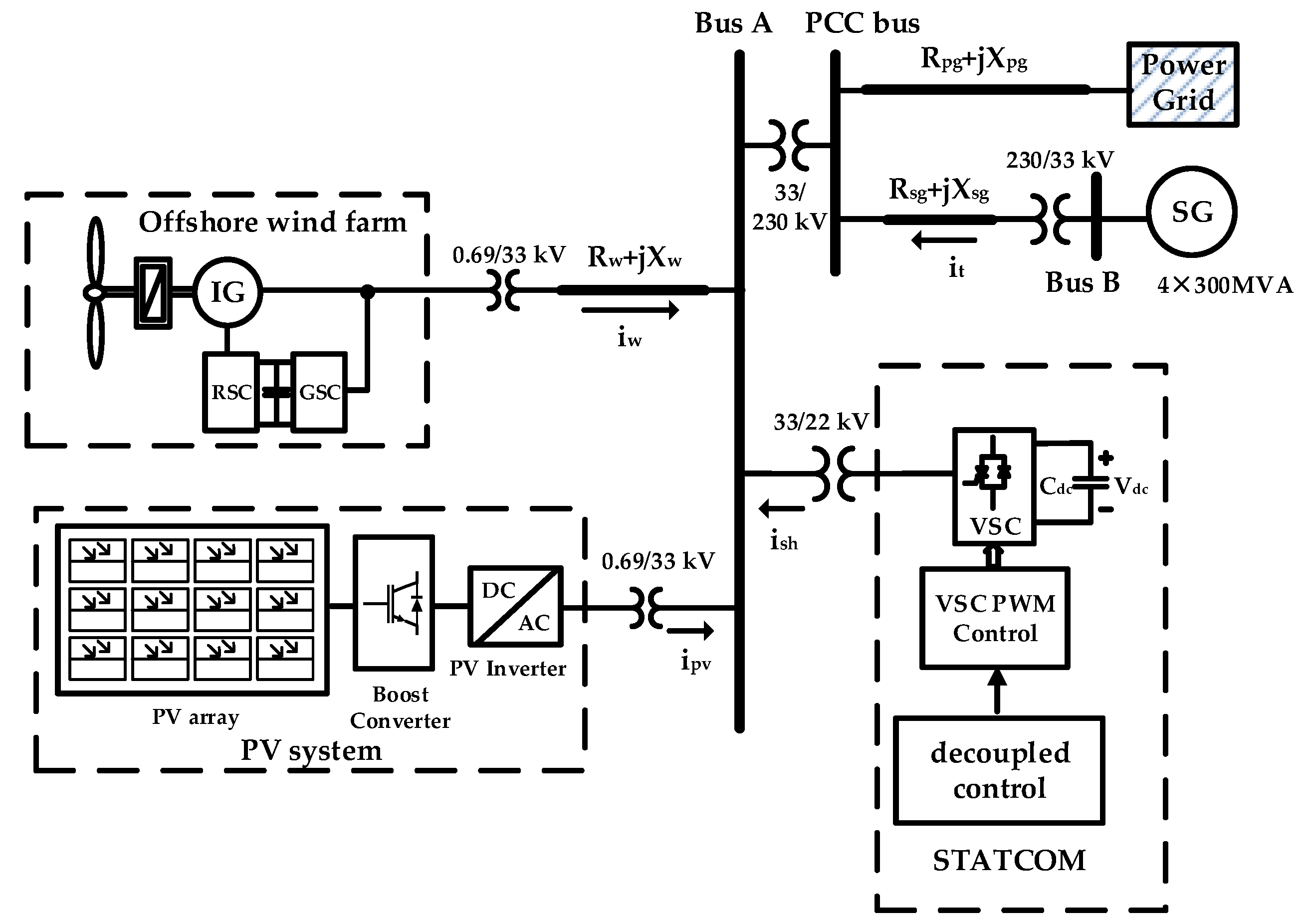
2. Analysis of the Studied System Models

The power grid diagram of the system configuration is shown in Figure 1. The system includes an integrated 80 MW large offshore wind farm (LSOWF) based on a doubly fed induction generator (DFIG), a 60 MW onshore large photovoltaic farm (LSPVF), a 50 MVAR STATCOM, and a 4 × 300 MVA synchronous generator (SG) connected to a power grid. A transmission line and a step-up transformer operating at 33/230 kV are used to connect four 300 MVA SGs operating in parallel to the power system. Connected to the common AC bus (bus A) is a LSOWF based on DFIG, a LSPVF, and a STATCOM. Using a 22/230 kV step-up transformer and cable, this bus is connected to the point of common coupling (PCC) bus. LSOWF’s wind turbines are represented by a DFIG, which includes an AC/DC converter, a DC link, a DC/AC inverter, and a 0.69/33 kV step-up transformer. The 60 MW onshore LSPVF is also connected to bus A through an equivalent aggregated DC/AC inverter. The STATCOM is connected to bus A through a 22/230 kV shunt transformer.

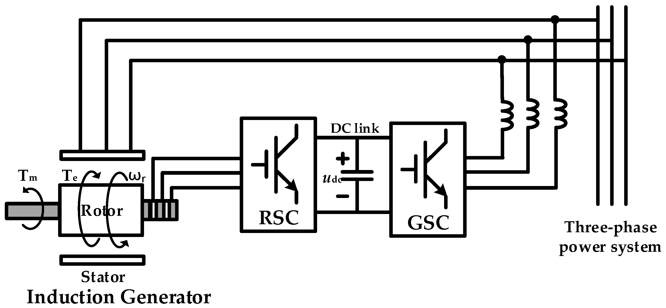
2.1. DFIG Mathematical Model

An illustration of a DFIG wind turbine’s system architecture can be found in Figure 2. There are two voltage source converters with pulse width modulation (PWM) power electronics connected to the wound rotor through a series of back-to-back power converters. The grid-side converter (GSC) is considered near the grid and the rotor-side converter (RSC) is considered near the rotor. There is a common DC interface between the RSC and GSC, and gearboxes and turbines are matched to form wind power generators. In order to support the DFIG’s operation, the stator of the unit is connected to the power supply of the system and the rotor is connected to a separate AC power supply with adjustable frequency, phase, and amplitude capabilities. If the frequency, phase, and amplitude of the rotor winding power supply are changed, the reactive power and rotational speed on the generator stator side can be changed. Using the rotor current to control and adjust virtual work can reduce the cost of virtual work compensation devices and increase system stability [8,11].

The primary purpose of the RSC is to control the real and reactive power output of the generator. The utility-side converter GSC mainly controls and stabilizes the voltage u_dc of its DC interface and provides real power to maintain a power factor equal to 1 pu. Three-phase systems have nonlinear voltage, U_s, and torque equations, T_e, so regulating the torque of induction generators is more complicated. Accordingly, the Park transformation for synchronous rotational coordinate conversion can be used to convert the originally balanced three-phase sine wave instantaneous value to the rotational coordinate d–q component. The DC components for the d- and q-axes can be changed and the three-phase sine wave peak value and phase angle can be controlled. Therefore, according to the literature [11], the stator/rotor voltage and fluxes of the d–q coordinate axis of the DFIG are shown in Equations (1)–(4). The electromagnetic torque equation is shown in Equation (5).

$$u_{s\_d,q}=R_s{i}_{s\_d,q}+\frac{d{\phi }_{s\_d,q}}{dt}+{\omega }_e{\phi }_{s\_d,q}$$

(1)

$$u_{r\_d,q}=R_r{i}_{r\_d,q}+\frac{d{\phi }_{r\_d,q}}{dt}+{({\omega }_e-n_p\omega }_r){\phi }_{r\_d,q}$$

(2)

$${\phi }_{s\_d,q}=L_s{i}_{s\_d,q}+L_{ms}{i}_{r\_d,q}$$

(3)

$${\phi }_{r\_d,q}=L_r{i}_{r\_d,q}+L_{mr}{i}_{r\_d,q}$$

(4)

$$T_e=\frac{3}{2}{n}_p{L}_{md}\left(i_{s\_q}{i}_{r\_d}-i_{s\_d}{i}_{r\_q}\right)$$

(5)

2.2. Mathematical Model of PV System

Photovoltaic (PV) modules are implemented using a PV array block. It is built from a series of modules connected in parallel and comprised of different strings, each consisting of a series of modules. The interior of a solar cell is composed of an equivalent current source, which is equivalent to N_pll parallel and N_se series diodes. It also has the equivalent series resistance, $R_s^{\prime }$, of solar cell output voltage and the equivalent resistance, $R_{sh}^{\prime }$, of the PN junction inside the solar cell terminal, as shown in Figure 3. Its electrical characteristics are affected by solar irradiance, solar cell material, ambient temperature, placement location, direction, and the latitude and longitude of the applied space. The equivalent output voltage, U_PV, and the equivalent output current, I_PV, are expressed as shown in Equations (6) and (7) [29,30]:

$$U_{PV}=\frac{DK{T}_p}{q}\mathrm{l}\mathrm{n}\left(\frac{N_{pll}{I}_{SC}}{I_{PV}}+1\right)$$

(6)

$$I_{PV}=N_{pll}{I}_{SC}-N_{pll}{I}_d\cdot \left\{exp\left[\frac{q\left(U_{PV}+I_{PV}{R}_s^{\prime }\right)}{DK{T}_p}\right]-1\right\}-\frac{U_{PV}+I_{PV}{R}_s^{\prime }}{R_{sh}^{\prime }}$$

(7)

where $R_s^{\prime }$ and $R_{sh}^{\prime }$ are the $\left(N_{se}/N_{pll}\right)\cdot R_S$ and the $\left(N_{se}/N_{pll}\right)\cdot R_{sh}$ of the series and the shunt resistance, respectively; q is the amount of charge contained in the electron (1.602 × 10⁻¹⁹ C); D is the ideal factor for solar energy material; and T_p is the ambient temperature of solar cells.

2.3. STATCOM Mathematical Model

Figure 4 depicts a STATCOM equivalent circuit and single line diagram. As part of the voltage source converter (VSC) system, pulse width modulation (PWM) technology generates a three-phase voltage source at the same frequency as the system through its pulse width modulation technology. Within one cycle of the AC power supply, the power electronic switching elements of the VSC are quickly switched to form an AC PWM voltage to reduce the subharmonic content. Changing the amplitude of the output voltage provides or absorbs reactive power for the system to maintain system voltage stability.

As shown in Figure 4, a STATCOM includes a DC interface capacitor, C_dc, a VSC, and a parallel coupled transformer, T_sh. The equivalent inductance, L_sh, is formed by combining the leakage inductance and filter inductance of T_sh and connecting them in series with the equivalent resistance, R_sh, in order to form the equivalent impedance, Z_sh. The STATCOM AC terminal circuit equation and DC interface equation use a Park transformation to transform a three-phase signal to a rotating reference frame as follows [16,17]:

$$\frac{d}{dt}\left[\begin{array}{c}{I}_{shd}\\ I_{shq}\end{array}\right]=\left[\begin{array}{cc}\frac{{-R}_{sh}}{L_{sh}}& {\omega }_0\\ {-\omega }_0& \frac{{-R}_{sh}}{L_{sh}}\end{array}\right]\left[\begin{array}{c}{I}_{shd}\\ I_{shq}\end{array}\right]+\frac{1}{L_{sh}}\left[\begin{array}{c}{V}_{shd}-V_{sd}\\ V_{shq}-V_{sq}\end{array}\right]$$

(8)

$$\frac{{dV}_{dc}}{dt}=\frac{-1}{C_{dc}}\left(I_{dc}+\frac{V_{dc}}{R_p}\right)$$

(9)

$$I_{dc}=m\left[I_{shd}\mathrm{s}\mathrm{i}\mathrm{n}\left({\delta }_s+\alpha \right)+I_{shq}\mathrm{c}\mathrm{o}\mathrm{s}\left({\delta }_s+\alpha \right)\right]$$

(10)

where $I_{shd}$ and $I_{shq}$ are the d–q axis current of the STATCOM injection system. $V_{shd}$ and $V_{shq}$ represent the d–q axis voltage of the STATCOM injection system, respectively. $V_{sd}$ and $V_{sq}$ describe the bus voltage of the d–q axis. $I_{dc}$ is the current of the STATCOM DC interface. $R_p$ is the equivalent resistance of the parallel DC interface. $m$ and $\alpha$ describe the modulation index and displacement of PWM. ${\delta }_s$ is the angle of the bus voltage, $V_s$.

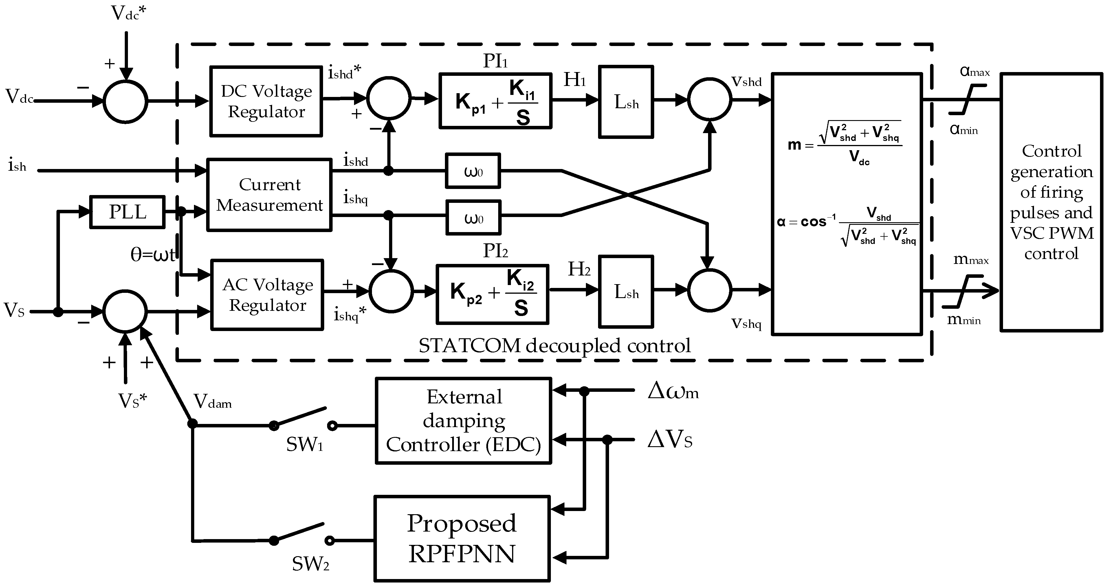
3. Design of the STATCOM Damping Controller

3.1. STATCOM Decoupled Control

An equivalent inductor, L_sh, connects the STATCOM’s output voltage, $V_{sh}$, to the bus voltage, $V_s$. Under steady-state operation, the system is not able to exchange real power with the STATCOM, so it can be assumed that $V_{sh}$ and $V_s$ are in phase. When there is a difference between the values of $V_{sh}$ and $V_s$ where the $V_{sh}$ is greater, a lagging current flows from the STATCOM into the bus. At this time, the STATCOM is in the capacitive mode, which provides system reactive power; conversely, when the output voltage, $V_{sh}$, value of the STATCOM is smaller than the bus voltage, $V_s$, value, it indicates that there is a leading current flowing into the bus from the STATCOM. At this time, the STATCOM is in inductive mode, i.e., it absorbs power from the system [2,15] for the purpose of obtaining decoupling control between the state variables. Since $V_{sd}$ and $V_{sq}$ are the constant values in the steady state, Equation (8) shows that controlling the voltage vector, $V_{shd}$, and $V_{shq}$ can change the magnitude of the compensating currents, $I_{shd}$ and $I_{shq}$, thereby achieving the goal of controlling real and virtual work. Due to the equation, $I_{shd}$ and $I_{shq}$ are multiplied by ${\omega }_0{L}_{sh}$. ${\omega }_0{L}_{sh}$ coupling is used as a decoupling control to simplify its operation. The detailed derivation of the decoupling control formula for a STATCOM can be found in [2], as shown in Equations (11) and (12):

$$v_{shd}=H_1{L}_{sh}-{\omega }_0{i}_{shq}+\left|v_s\right|$$

(11)

$$v_{shq}=H_2{L}_{sh}-{\omega }_0{i}_{shd}$$

(12)

In Figure 5, a block diagram of a STATCOM’s control system is presented. Among the components of this model, H₁ is the state variable from the d axis and H₂ is the state variable from the q axis, and are used to represent the outputs of the real and reactive current regulators in the STATCOM controller, while the outputs of the proportional integral controllers, PI₁ and PI₂, become the H₁ and H₂ variables. At this time, the $i_{shd}$ and $i_{shq}$ currents can be independently controlled by H₁ and H₂, respectively. According to the feedback control law, taking PI₁ and PI₂ as inputs for the H₁ and H₂ control variables, a proportional integral controller can be used to adjust $i_{shd}$ and $i_{shq}$ to achieve the target value. The system captures the three-phase bus voltage, $V_s$, and obtains the system angle, θ, through a phase-locked circuit (PLL). The captured three-phase current, I_sh, is measured through a current meter. I_sh and the system angle, θ, are used obtain the q-axis and d-axis currents ($i_{shq}$ and $i_{shd}$) through a current measuring device. After comparing the error signals of $i_{shd}$ and $i_{shq}$ with the reference values $i_{shd}^{\mathrm{*}}$ and $i_{shq}^{\mathrm{*}}$, the converter output voltage values, $v_{shd}$ and $v_{shq}$, can be obtained through PI₁ and PI₂ outputs and decoupling processing. In practical applications, to control the output of STATCOM converters, the $v_{shd}$ and $v_{shq}$ must be converted into trigger signals for the converter phase angle, α, and modulation index, m.

3.2. The External Damping Controller of STATCOM

As shown in Figure 5, this paper uses an external damping controller (EDC) in the control loop of the bus voltage to provide additional damping signals to improve the unstable low-frequency electromechanical oscillation mode of the system. The EDC is composed of two sets of lead-lag controllers, a washout filter and a limiter. Its input signals are the bus voltage difference, ΔV_S, and the synchronous generator speed difference Δω_SG [2]. In the EDC, eigenvalues are analyzed using a theory of modal control to determine their complex eigenvalues. In [31,32] the matrices of the state space and the transfer function are listed.

$$\dot{\mathbf{X}}=\mathbf{A}\mathbf{X}+\mathbf{B}\mathbf{R}$$

(13)

$$\mathbf{Y}=\mathbf{C}\mathbf{X}+\mathbf{D}\mathbf{R}$$

(14)

Here, X and $\dot{\mathbf{X}}$ are the matrices containing the state variables as well as the differential operators associated with them. Matrix R represents plant inputs. The value of Y corresponds to the value of ${\mathsf{\Delta }V}_{dam}$ in the system. The constants A, B, C, and D are the state matrix, control matrix, output matrix, and transmission matrix of the system, respectively. This is a vector of the substates X = [X_DFIG, X_WT, X_TS, X_PV, X_SATCOM]^T = [$u_{s\_d,q}$ $u_{r\_d,q}$ ${\phi }_{s\_d,q}$ ${\phi }_{r\_d,q}$ ${\omega }_e$ ω_SG V_S ${\omega }_0$ $U_{PV}$ $I_{SC}$ $I_{shd}$ $I_{shq}$ $V_{dc}$]^T, where X_DFIG is the state vector of DFIG, X_WT is the state vector of the wind turbine mechanical system, X_TS is the state vector of the SG and transformer, X_PV is the state vector of the PV system, X_STATCOM is the state vector of the STATCOM system, and R is the input vector, where R = [ΔV_S, Δω_SG]. Therefore, the transfer function can be written as shown in Equation (15):

$$\mathrm{T}\left(\mathrm{s}\right)=\frac{\mathbf{Y}\left(\mathbf{s}\right)}{\mathbf{R}\left(\mathbf{s}\right)}=\frac{S{K}_1{K}_2}{1+S{T}_m}\left[\frac{T_{d2}}{K_1(1+S{T}_{d2})}+\frac{T_{d1}}{K_2(1+S{T}_{d1})}\right]$$

(15)

The EDC is composed of two sets of lead-lag controllers, a washout filter and a limiter. For a detailed block diagram, refer to [2]. In Equation (15), T_d1 and T_d2 are the time constant of the two washout filters. Washout filters are stable high-pass filters with no static gain. In this way, low frequency input signals are filtered out, leaving steady state outputs unaffected. K₁, K₂, T_m are the lead-lag controller compensation gains and sampling period. These parameters allow the lead-lag compensator to improve undesirable frequency responses.

In order to obtain the algebraic equation of a closed-loop system including an EDC, the Laplace transform can be applied to Formulae (8) and (9).

Table 1. The system eigenvalues for a STATCOM without/with EDC.

Eigenvalues	STATCOM without EDC	STATCOM with EDC
λ1	−43.27 ± j4393.62	−43.27 ± j4393.62
λ2	−106.73 ± j414.67	−106.70 ± j414.67
λ3	−76.36 ± j92.83	−70.63 ± j136.09
λ4	−53.34 ± j2.17	−53.54 ± j2.40
λ5	−0.14, −40.60	−0.209, −40.64
λ6	−9.96 ± j28.42	−9.92 ± j28.35
λ7	−0.286 ± j10.22 [0.37]	−1.88 ± j12.32 [0.51]
λ8	−10.89 ± j2.68	−10.83 ± j2.71
λ9	−6.17, −3.20	−6.08, −2.44
λ10	−0.78 ± j1.63 [0.51]	−0.82 ± j1.43 [0.88]
λ11	−1.01, −0.09	−1.01, −0.09
λ12	−100.12	−100.12

shows the system eigenvalues calculated from the A matrix for analyzing this closed loop system. The eigenvalues λ₁–λ₂, λ₃–λ₅, λ₆–λ₈, λ₉–λ₁₀ and λ₁₁–λ₁₂ listed in Table 1. The eigenvalues λ₁–λ₂ refer to the mechanical mode of the DFIG. The eigenvalues λ₃–λ₅ are the wind turbine’s mechanical mode. The eigenvalues λ₆–λ₈ correspond to the exciter mode of the studied SG, respectively. The eigenvalues λ₉–λ₁₀ refer to the electrical mode of the PV system. The eigenvalues λ₁₁–λ₁₂ are the electrical mode of the STATCOM. The EDC parameters are calculated by substituting the two pairs of complex conjugate eigenvalues (λ₇ and λ₁₀). From the table, it can be observed that when the STATCOM did not have an EDC, the eigenvalues were λ₇ = −0.286 ± j10.22 and λ₁₀ = −0.78 ± j1.63, indicating that the damping of this mode is worse than other eigenvalues. Consequently, the pole with poor damping is moved to a position with better damping by the EDC λ₇ = −1.88 ± j12.32 λ₁₀ = −0.82 ± j1.43, and then the system parameters K₁ = 26.48, K₂ = 30.16, T_d1 = 0.75, T_d2 = 0.58, and T_m = 0.64 are derived from the equation. It can also be observed from the table that all eigenvalues of the STATCOM functions fall on the left side of the complex plane after the EDC has been configured. The damping ratios of λ₇ and λ₁₀ also increased from 0.37 and 0.51 to 0.51 and 0.88, thereby reducing system oscillation.

4. Recurrent Petri Fuzzy Probabilistic Neural Network

The Petri NN is a composite model that can be represented graphically. A wide range of computer systems have been analyzed and designed using it. It can be used to describe and analyze the concurrent processing of multiple events in dynamic systems. The work of a recurrent Petri fuzzy probabilistic neural network (RPFPNN) is mainly divided into the output calculation of the feedforward process and the weight adjustment and error generation stage of the feedback process. The RPFPNN generates the gains V_dam.

4.1. Feedforward Process

The RPFPNN structure is shown in Figure 6 and is divided into five layers and a feedback link. The first layer is the information transmission layer, which is only used for information transmission. Therefore, the weights of this layer do not require training and are set to 1. There are two neuron nodes in this layer. The output, $F_P^{\left(1\right)}$, of this layer is the signal of the input signal plus the output value, $O_m^{\left(6\right)}$, via a delay time of z⁻¹ of the last layer, as shown in Equation (16):

$$F_P^{\left(1\right)}\left(k\right)=N_P^{\left(1\right)}\left(k\right)+O_m^{\left(6\right)}(k-1)\cdot {\mu }_P, P=1,2$$

(16)

where $N_P^{\left(1\right)}$ is the signal that is fed into the first layer’s Pth node, which, respectively, refers to ∆V_S and ∆ω_SG. N represents the number of times the iteration has been performed. ${\mu }_P$ represents the weights of the feedback layers of the RPFPNN. The ${\mu }_P$ is also a factor which must be trained for the network.

Because the RPFPNN introduces the concept of a fuzzy system, the output signal of the first layer needs to be established as a Gaussian function in the second layer. The second layer’s output value equation, $M_U^{\left(2\right)}$, for connecting the Pth neuron in the first layer to the Uth neuron in the second layer is shown in Equation (17):

$$M_U^{\left(2\right)}(F_P^{\left(1\right)})=e^{-\frac{{\left(F_P^{\left(1\right)}\left(k\right)-a_U\right)}^2}{b_U^2}}, U=1, 2\dots 7$$

(17)

where a_U and b_U are the parameters to be trained for the Gaussian function and also represent the weights of this layer.

This Petri net model extends the stochastic Petri net model to accommodate Gaussian distributions. An interval of time between the transition ignition and implementation process is also modeled using a Gaussian distribution, which simulates the implementation process with variable time intervals. The operating mechanism of the Petri layer first generates the identification evolution sequence and transition initiation sequence of the model through the initiation of transitions in the model, thereby reflecting the dynamic characteristics of the Petri net model. Assuming that the transition value, $T_r$, in the Petri layer is 1, it is fired, and vice versa. The input, $n_T^{\left(3\right)}$, and output value, $F_T^{\left(3\right)}$, of the third layer are expressed as shown in Equations (20) and (21):

$$T_r(k)=\left\{\begin{array}{c}1, { M}_U^{\left(2\right)}\ge {\beta }_U\\ 0,{ M}_U^{\left(2\right)}<{\beta }_U\end{array} \right., U=1, 2\dots 7$$

(18)

$${\beta }_U=\frac{ϵ\cdot e^{-\rho \xi }}{1-e^{-\rho \xi }}$$

(19)

$$n_T^{\left(3\right)}(k)=\{\begin{array}{c}{ M}_U^{\left(2\right)}\left(\mathrm{k}\right),\hspace{1em}{T}_r\left(\mathrm{k}\right)=1\hfill \\ 0,\hspace{1em}\hspace{1em}\hspace{1em}\hspace{1em}{T}_r\left(\mathrm{k}\right)=0\hfill \end{array}$$

(20)

$$F_T^{\left(3\right)}(k)=f(n_T^{\left(3\right)}(k))$$

(21)

where ${\beta }_U$ represents energy threshold value of the time obedience index. $\xi$ is the average value of ∆V_S and ∆ω_SG ${\left(abs\left(\mathsf{\Delta }{\mathrm{V}}_{\mathrm{S}}\right)+abs\left(\mathsf{\Delta }{\mathsf{\omega }}_{\mathrm{S}\mathrm{G}}\right)\right)}^{-1}$. $ϵ$ and $\rho$ are the positive coefficients of the threshold parameter.

The fifth layer is the sample layer of the probability net, called the probability layer. Based on training samples, the probability density function of neurons in this layer is estimated through Parzen estimation of Gaussian kernels. Based on the estimation of kernel probability density, various probability estimates can be obtained by normalizing the output layer, as shown in Equation (22).

$$P_l^{\left(4\right)}(F_T^{\left(3\right)})=e^{-\frac{{\left(F_T^{\left(3\right)}\left(k\right)-{{\rm Y}}_{Tl}\right)}^2}{{\sigma }_l^2}}, l=1, 2\dots 7$$

(22)

Here, ${\sigma }_l^{}$ represents a smoothing parameter. It is half of the average distance between eigenvectors in the same group. ${{\rm Y}}_{Tl}$ is a training sample that belongs to the Tth neuron of the previous layer and is connected to the kth neuron of this layer. A probability layer is a useful method in this paper since linear learning algorithms can be used to accomplish nonlinear learning algorithms’ tasks while maintaining their accuracy and other characteristics. Since the weights associated with this network represent the distribution of pattern samples, it is not necessary to train the ${\sigma }_l$ and ${{\rm Y}}_{Tl}$ of the network, as they can meet the real-time processing requirements during training.

Because the probability layer requires a high representativeness of training samples, a fuzzy layer is added. By utilizing the characteristics of fuzzy rules, the requirements of training samples are summarized. The triggering force of fuzzy rules with high intensity is greater, while the triggering force of fuzzy rules with low intensity is smaller. Based on the fuzzy firing strength that is generated by this layer, the preconditions are matched based on the input triggers to this layer. As an alternative to the MIN operation used for the operation of the simple algebraic product, either the matching operation or the fuzzy AND aggregation operation was chosen instead. $\mathsf{\Pi }$ is the symbol that is used to represent each node in this layer, which generates j term rules.

After passing through the rule layer, the final output layer is entered. Throughout the output layer, nodes are referred to as output language nodes. Defuzzification operations are performed in this layer. Each node outputs a linear combination of the results that are obtained by combining the results produced by each rule. During this layer, nodes are labelled and the output of the layer is calculated as the sum of all signal inputs. The neuron outputs, $R_j^{\left(5\right)}$ and $O_m^{\left(6\right)}$, of the rule and output layers are expressed as shown in Equations (23) and (24).

$$R_j^{\left(5\right)}(k)=\prod _{\mathrm{l}}{P}_l^{\left(4\right)}\left(k\right)\cdot w_{lj}\cdot \prod _U{M}_U^{\left(2\right)}\left(k\right)\cdot w_{Uj}$$

(23)

$$O_m^{\left(6\right)}\left(k\right)=R_j^{\left(5\right)}\left(k\right)\cdot w_m$$

(24)

Here, $w_{Uj}$, between the probability layer and the rule layer, is designed to be a unity. $w_{Uj}$ is also set to be a unity between the membership layer and the rule layer, $j\in (1,2,3,...,l\times U)$. The link weight, $w_m$, is the output action strength of the output signal associated with the jth rule.

4.2. Feedback Process

The tuning parameters in the RPFPNN are standard deviation, STD b_U; the average value, a_U, of the seconf layer; the output layer weight, $w_m$; and the feedback layer weight, ${\mu }_P$. Usually, an RPFPNN is designed based on the previously introduced PFPNN structure and additional feedback units to increase the dynamic behavior of the network. The feedforward design of the RPFPNN is simple and very direct. Although the RPFPNN structure proposed in this paper has six layers, only four weights need to be trained. However, the operation of the backpropagation algorithm, i.e., error transformation, can have an adverse effect on the performance of the system. The delta learning algorithm is adopted [18] in this paper and the cost function, E, for the delta learning algorithm can be formulated as shown in Equation (25):

$$E=\sum _{\mathrm{n}}{e}_n^2\left(k\right)=\frac{1}{2}\sum _{\mathrm{n}}{\left(d_n\right(k)-{\Gamma }_n(k\left)\right)}^2$$

(25)

where $e_n^{}\left(k\right)$ represents the error of the nth neuron at the kth learning time; $d_n\left(k\right)$ represents the desired output of the nth neuron at the kth learning time; ${\Gamma }_n\left(k\right)$ represents the internal excitation status of the nth neuron at the kth learning time; and $f(\cdot )$ represents the activation function in the nth membership function.

An equation that can be used to calculate the error term to be propagated is shown in Equations (26)–(28) [1,3]:

$${\delta }_m=-\frac{\partial E}{\partial O_m^{\left(6\right)}}=-\frac{\partial E}{\partial e_n^{}}\frac{\partial e_n^{}}{\partial {\Gamma }_n}\frac{\partial {\Gamma }_n}{\partial O_m^{\left(6\right)}}$$

(26)

$${\delta }_j=-\frac{\partial E}{\partial R_j^{\left(5\right)}}=-\frac{\partial E}{\partial O_m^{\left(6\right)}}\frac{\partial O_m^{\left(6\right)}}{\partial R_j^{\left(5\right)}}={\delta }_m{\cdot w}_m$$

(27)

$${\delta }_M=-\frac{\partial E}{\partial M_U^{\left(2\right)}}=-\frac{\partial E}{\partial O_m^{\left(6\right)}}\frac{\partial O_m^{\left(6\right)}}{\partial R_j^{\left(5\right)}}\frac{\partial R_j^{\left(5\right)}}{\partial M_U^{\left(2\right)}}=\sum _j{\delta }_j{\cdot M}_U^{\left(2\right)}\left(k\right){\cdot w}_{Uj}$$

(28)

In order to minimize the difference between the desired and actual outputs, the backpropagation algorithm iteratively reduces the difference (or error) based on this principle. During each iteration, the backpropagation algorithm adjusts the parameters and weights to reduce the error. The RPFPNN proposes four parameters to be trained in the proposed model, a_U, b_U, $w_m$, and ${\mu }_P$. The formula for adjusting parameters is obtained from:

$$\mathsf{\Delta }{w}_m=-{\eta }_w\frac{\partial E}{\partial u_m^{\left(6\right)}}\frac{\partial u_m^{\left(6\right)}}{\partial {\Gamma }_n}\frac{\partial {\Gamma }_n}{\partial w_m}={\eta }_w{\delta }_m{O}_m^{\left(6\right)}$$

(29)

$$\mathsf{\Delta }{a}_U=-{\eta }_a\frac{\partial E}{\partial a_U}=-{\eta }_a\frac{\partial E}{\partial O_m^{\left(6\right)}}\frac{\partial O_m^{\left(6\right)}}{\partial u_m^{\left(6\right)}}\frac{\partial u_m^{\left(6\right)}}{\partial M_U^{\left(2\right)}}\frac{\partial M_U^{\left(2\right)}}{\partial u_U^{\left(2\right)}}\frac{\partial u_U^{\left(2\right)}}{\partial a_U}={\eta }_a{\delta }_M\frac{{2(F}_P^{\left(1\right)}-a_U)}{b_U^2}$$

(30)

$$\mathsf{\Delta }{b}_U=-{\eta }_b\frac{\partial E}{\partial b_U}=-{\eta }_b\frac{\partial E}{\partial O_m^{\left(6\right)}}\frac{\partial O_m^{\left(6\right)}}{\partial u_m^{\left(6\right)}}\frac{\partial u_m^{\left(6\right)}}{\partial M_U^{\left(2\right)}}\frac{\partial M_U^{\left(2\right)}}{\partial u_U^{\left(2\right)}}\frac{\partial u_U^{\left(2\right)}}{\partial b_U}={\eta }_b{\delta }_M\frac{{{2(F}_P^{\left(1\right)}-a_U)}^2}{b_U^3}$$

(31)

$$\begin{array}{cc}\hfill \mathsf{\Delta }{\mu }_P=-{\eta }_{\mu }\frac{\partial E}{\partial {\mu }_P}& =-{\eta }_{\mu }\frac{\partial E}{\partial O_m^{\left(6\right)}}\frac{\partial O_m^{\left(6\right)}}{\partial u_m^{\left(6\right)}}\frac{\partial u_m^{\left(6\right)}}{\partial M_U^{\left(2\right)}}\frac{\partial M_U^{\left(2\right)}}{\partial u_U^{\left(2\right)}}\frac{\partial u_U^{\left(2\right)}}{\partial F_P^{\left(1\right)}}\frac{\partial F_P^{\left(1\right)}}{\partial {\mu }_P}\hfill \\ & ={\displaystyle \sum _U}{\eta }_{\mu }{\delta }_M\frac{2\left(a_U-F_P^{\left(1\right)}\right)}{b_U^2}{\cdot N}_P^{\left(1\right)}{O}_m^{\left(6\right)}(k-1)\hfill \end{array}$$

(32)

where u is the input signal of its layer of neurons and ${\eta }_w$, ${\eta }_a$, ${\eta }_b$, and ${\eta }_{\mu }$ are the small constants greater than zero, referred to as the learning rate of the $\mathsf{\Delta }{w}_m$, $\mathsf{\Delta }{a}_U$, $\mathsf{\Delta }{b}_U$, and $\mathsf{\Delta }{\mu }_P$.

The all-purpose learn by induction rule is updated by the following mathematical formula (33)–(36):

$$w_m(k+1)=w_m\left(k\right)+\mathsf{\Delta }{w}_m\left(k\right)$$

(33)

$$a_U(k+1)=a_U\left(k\right)+\mathsf{\Delta }{a}_U\left(k\right)$$

(34)

$$b_U(k+1)=b_U\left(k\right)+\mathsf{\Delta }{b}_U\left(k\right)$$

(35)

$${\mu }_P(k+1)={\mu }_P\left(k\right)+\mathsf{\Delta }{\mu }_P\left(k\right)$$

(36)

Backpropagation (BP) algorithms can break down if they have a very large or very small learning rate. It has been argued that a low learning rate will make the network learn slowly, whereas a high learning rate may result in a divergence between the weights and objective functions of the network. Therefore, the learning rate has to be selected very carefully. Properly adjusting the ${\eta }_w$, ${\eta }_a$, ${\eta }_b$, and ${\eta }_{\mu }$ can also modify the convergent speed of the network.

It is possible for BP algorithms to fail if they experience relatively high or low learning rates. A network with a low learning rate may be able to learn slowly, whereas a network with a high learning rate may be able to diverge between the weights and objective functions. Therefore, it is necessary to choose the learning rate very carefully. Appropriate adjustments can also change the convergence speed of the network. In order to ensure the convergence of the tracking error, the learning rate chosen for the discrete Lyapunov function as described in [33] must be determined according to Equations (37)–(40):

$${\eta }_w=\frac{1}{2}{\left(\sum _{\mathrm{m}}{\left(\frac{\partial {\Gamma }_n}{\partial w_m}\right)}^2+\varphi \right)}^{-1}$$

(37)

$${\eta }_a=\frac{1}{2}{\left(\sum _{\mathrm{U}}{\left(\frac{\partial {\Gamma }_n}{\partial a_U}\right)}^2+\varphi \right)}^{-1}$$

(38)

$${\eta }_b=\frac{1}{2}{\left(\sum _{\mathrm{U}}{\left(\frac{\partial {\Gamma }_n}{\partial b_U}\right)}^2+\varphi \right)}^{-1}$$

(39)

$${\eta }_{\mu }=\frac{1}{2}{\left(\sum _{\mathrm{P}}{\left(\frac{\partial {\Gamma }_n}{\partial {\mu }_P}\right)}^2+\varphi \right)}^{-1}$$

(40)

where $\varphi$ is a small positive number.

5. Time-Domain Simulations and Discussion

As a result of the nonlinear simulation model of this system, MATLAB/SIMULINK 2016b software has been implemented for the system simulation. The proposed STATCOM was tested using an RPFPNN control to verify its robustness and a comparison was made between a STATCOM using an EDC as a damping controller (as shown in Section 3.2) and a STATCOM without an EDC. Firstly, suppose that the DFIG-based LSOWF operates stably at a basic wind speed of 12 m/s. According to the LSPVF model, the irradiance is assumed to be 1000 W/m² and the temperature is assumed to be 30 °C. The power grid parameters are shown in

Table 2. Simulation parameters of the power grid.

System
Vbase = 230 kV; Sbsae = 10 MVA; ST = 8 MVA; VTH = 230 KV; VTL = 33 KV; Vgrid = 1 pu; Z% = 2.5; RT= 0.00083 pu; XT = 0.025 pu; Rpg = 0.042 pu; Xpg = 0.85 pu; Rsg = 0.021 pu; Xsg = 0.425 pu; Rw = 0.0072 pu; Xw = 0.172 pu; Ron = 1 mΩ; Rg = 1 mΩ

and the other parameters are in Appendix A.

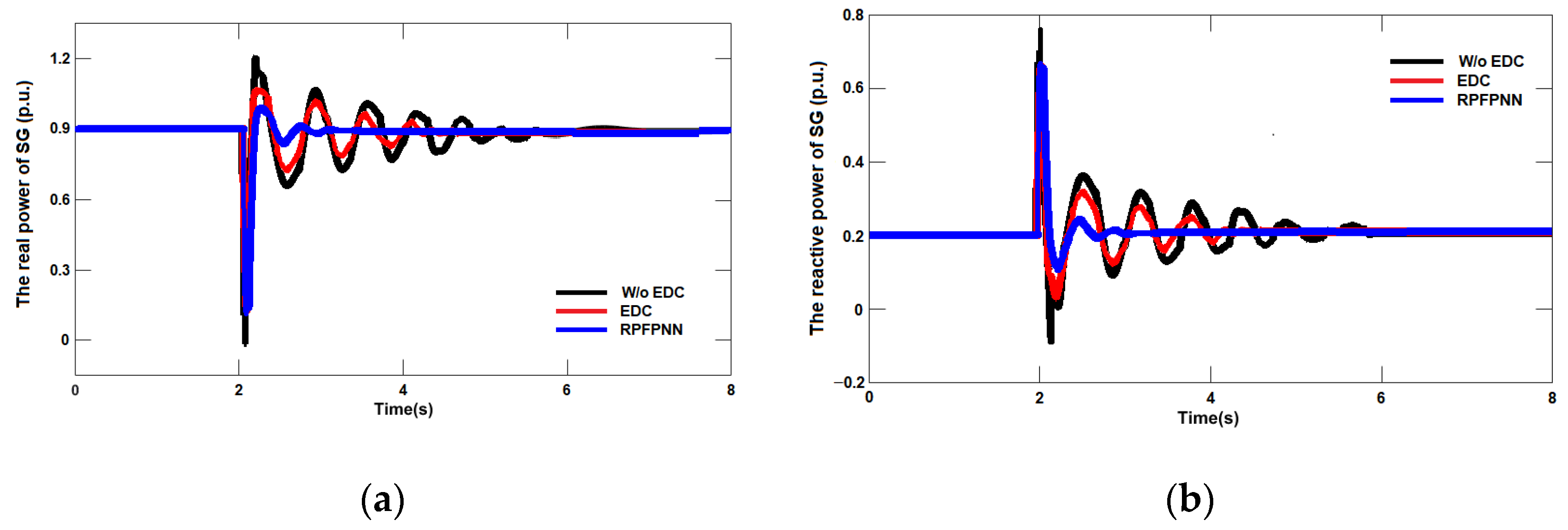
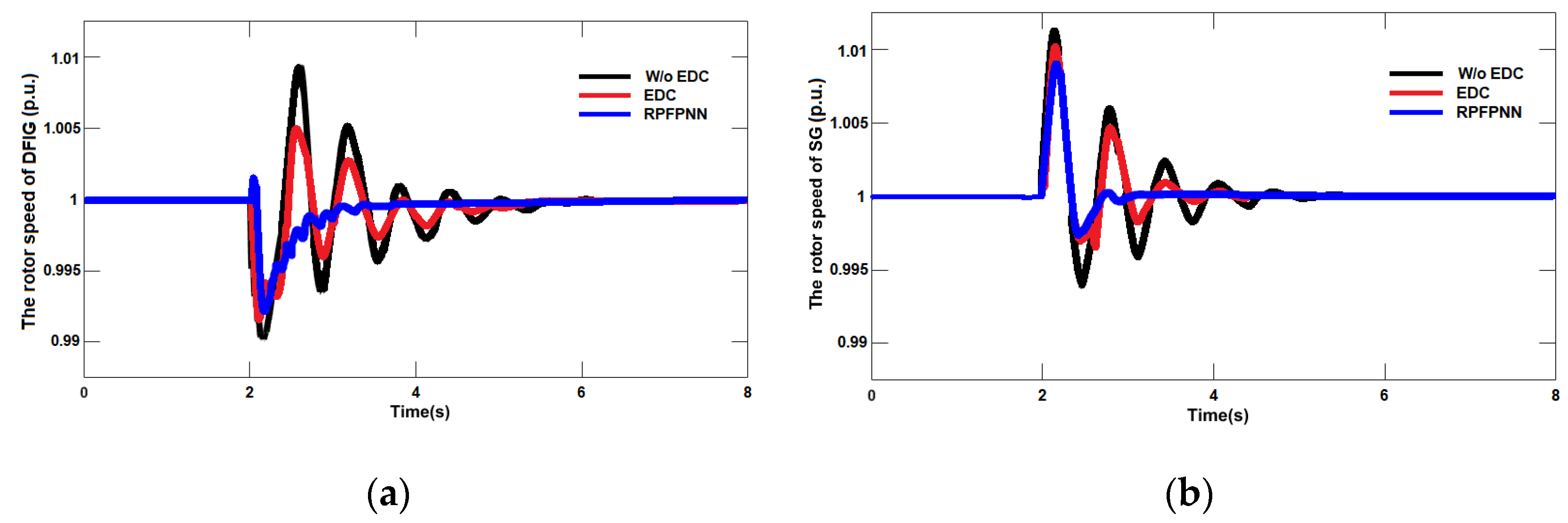
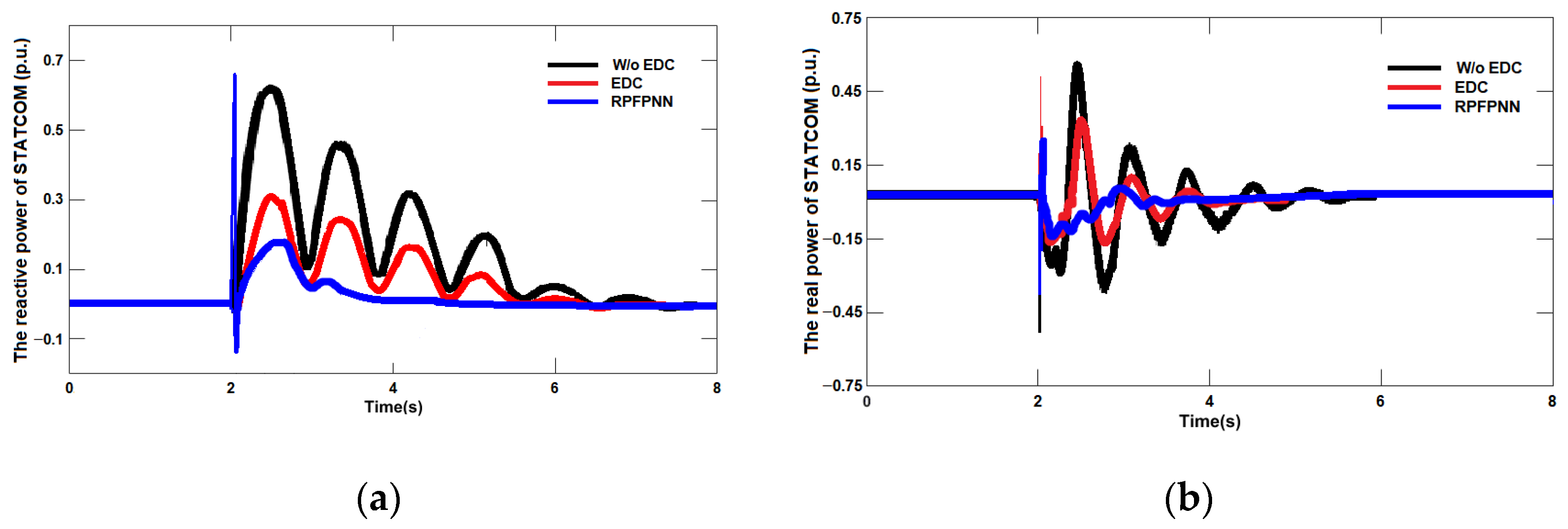
5.1. Case 1: The Transient Response to a Three-Phase Short Circuit Fault

This simulation assumes that a three-phase short circuit to ground fault suddenly occurs on the PCC bus at 2 s, with a fault time of 0.1 s. The fault is cleared at 2.1 s and the fault resistance is 1 mΩ. The STATCOM of the system model is an IGBT-diode bridge structure with a C_dc of 2200 μF and a DC voltage of 800 V. Other detailed parameters are shown in Appendix A.

During a fault, both the wind farm and the photovoltaic farm suffer serious power interruptions. As shown in Figure 7, the DFIG-based LSOWF shows transient response diagrams for real power and reactive power. As shown in Figure 8, the LSPVF shows transient response diagrams for real and reactive power. It is evident that a STATCOM with an RPFPNN controller is able to achieve the minimum fluctuations in both real and reactive power in the event of a fault, as shown in Figure 7a,b, showing real power and reactive power in response to the DFIG-based LSOWF. This enables it to converge to steady-state operation the fastest. The damping controller of the STATCOM combined with an EDC is second. The STATCOM can stabilize system oscillations, but the transient control response of the STATCOM with only traditional internal controllers without an EDC is the worst. From the figures, it can be observed that the overshoot and the undershoot of the real and the reactive power after fault clearing is the highest, with convergence times of 6.9 s and 6 s, respectively. Figure 8a,b, respectively, plot the responses of the real power and reactive power of the LSPVF. Furthermore, the STATCOM with an RPFPNN controller can achieve the minimum fluctuation of real and reactive power, converging to steady-state operation in approximately 2.8 s and 3 s, respectively. The slowest convergence is observed in the traditional STATCOM. From the graph, it can be seen that after the fault is cleared, the overshoot and undershoot of real and reactive power are the highest, with convergence times of 5.8 s and 6 s, respectively.

Figure 9a,b show the real and reactive power response diagrams provided by synchronous generation. When the fault is cleared, the generator’s speed is still different from the rated speed. The power angle will also oscillate further, causing the real power and reactive power to oscillate, and the system will lose stability. Figure 9 clearly illustrates the impact of a STATCOM with/without EDC: the damping of the studied system is poor and the stability time is between 7 s and 6 s. When the designed RPFPNN controller is used in a STATCOM, the system has better damping and converges when the stability time is approximately 3 s. The transient response diagram of the DFIG and SG rotor speed is presented Figure 10a,b. The fault occurs when the generator rotor oscillates between the generator rotors due to insufficient damping and negative damping. As shown in Figure 10, the STATCOM with an RPFPNN controller can obtain the minimum rotor speed of the DFIG and SG and converge to steady-state operation in the fastest time. The damping controller of the STATCOM combined with an EDC is second. The STATCOM can stabilize system oscillations, but the transient control response of the STATCOM with only traditional internal controllers without an EDC is the worst.

Figure 11a,b show the DC voltage responses of the PV system and the PCC AC bus. It can also be seen that the STATCOM with an RPFPNN controller can achieve the minimum fluctuation of voltage. The DC voltage of the PV system converges to steady-state operation in approximately 3.1 s, while for PCC bus voltage it takes approximately 3.3 s. The slowest convergence is observed in the traditional STATCOM. From the graph, it can be seen that after the fault is cleared, the overshoot and undershoot of the voltage are the highest, with convergence times of 6.3 s and 6.4 s, respectively. The STATCOM provides reactive power in response to a serious short-circuit fault that has occurred in the system, as shown in Figure 12a, in order to maintain the bus voltage. The proposed RPFPNN controller is also observed to be the most effective in terms of performance, followed by the STATCOM with an EDC, while the STATCOM without an EDC has the worst oscillation and convergence time. It can be seen in Figure 12b that the STATCOM requires very small active power for real charging and discharging to maintain its capacitor voltage. In addition, the proposed RPFPNN controller has the highest vibration suppression effect for achieving STATCOM stable charging and discharging DC voltage.

In Case 1, under a severe three-phase short-circuit fault, the proposed RPFPNN combined with a STATCOM as a system damping controller showed the best damping characteristics, which were better than the EDC in the literature [14], and could effectively suppress the large regeneration transient oscillation phenomenon when energy was connected to the grid.

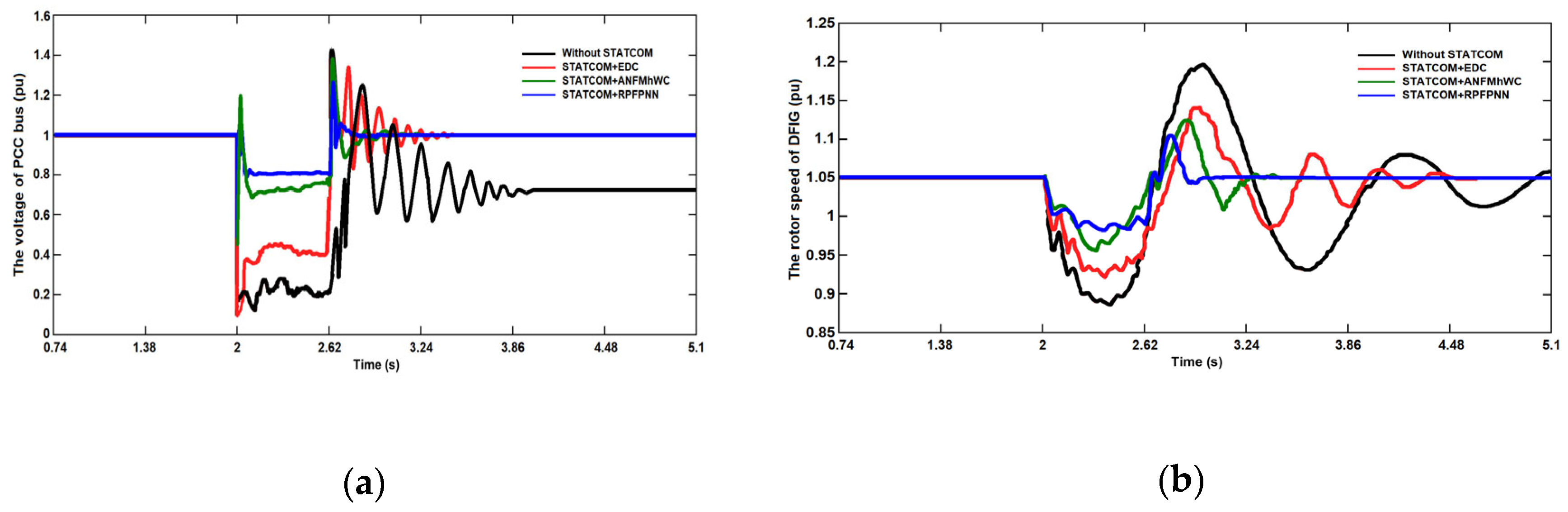
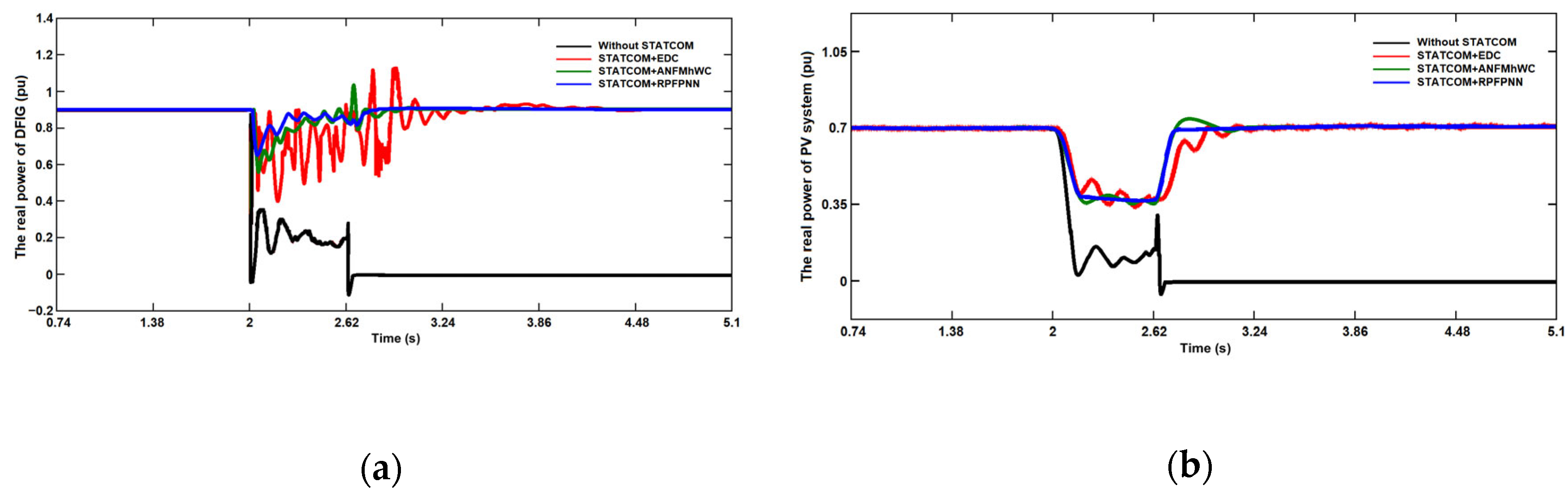
5.2. Case 2: The Fault Ride-Through Performance

This case cites Taiwan’s regulations [34]. It is essential that renewable energy fields have low-voltage ride-through capabilities that can maintain grid-connected operation for 620 ms at 20% of their rated voltage. Therefore, this case assumes that the LSOWF and LSPVF are fully loaded, that the voltage drop depth is 80% of the grid’s rated voltage in 2 s, and that it returns to the rated voltage after 620 ms. It is stable before the grid drops. For the purpose of further verifying the robustness of the RPFPNN proposed in this paper, an ANFMhWC [25] has been added to further verify its robustness.

As shown in Figure 13a, the STATCOM + RPFPNN has a superior fault ride-through capability when the voltage drops by 80%. It also has the smallest overshoot after the fault is cleared and the fastest return to the voltage rating. The second best is the STATCOM + ANFMhWC. The STATCOM + EDC can also ride through faults; however, after the fault is cleared, it will continue to oscillate for a period of time before converging. In the figure, it can be seen that if there is no STATCOM because there is no fault in the LSOWF and LSPVF ride-through capability, when a large fault that lasts for a period of time occurs, causing the LSOWF and LSPVF to be disconnected from the grid, the PCC voltage cannot return to the voltage rating, which may cause the grid to collapse. Figure 13b shows DFIG rotor speed. It has been found that when a STATCOM is not installed, the DFIG rotor speed oscillates greatly due to wind farm disconnection. However, the STATCOM + RPFPNN converges faster than other control methods after the fault is cleared.

Figure 14a,b show the active powers of LSOWF and LSPVF. From the figure shown, it is clear that when the STATCOM + RPFPNN is used, the oscillation of real power can be better suppressed during and after a fault. The LSOWF and LSPVF are automatically disconnected if there is no STATCOM due to a low-voltage fault where real power cannot be recovered because the LSOWF and LSPVF are disconnected. This represents a failure to meet the requirements in terms of fault ride-through capability that have been set forth by the Taiwan Power Company. Figure 15a,b show that without a STATCOM, the LSOWF and LSPVF inject a reactive power of 0.2 and 0.3 pu before disconnection, while after disconnection, there is no reactive power due to the shutdown. The STATCOM + RPFPNN allows for maximum reactive power to be injected into the grid in order to assist in grid recovery. It has smoother output, a faster convergence time, and minimal oscillations in reactive power.

6. Conclusions and Future Works

Renewable energy power generation is unstable due to its intermittent nature. Especially when the power grid fails, the integration of renewable energy into the existing power grid will cause transient fluctuations in the system. This may further cause power outages or system collapses. To achieve power fluctuation suppression and damping improvement, this paper presents the dynamic stability improvement of an integrated LSOWF and LSPVF using a STATCOM. An RPFPNN damping controller has been designed for the STATCOM and the detailed design of the STATCOM damping controller has been completed. In simulations of a three-phase short circuit occurring on the PCC bus of the system, the proposed RPFPNN of the STATCOM is shown to effectively suppress the inherent oscillations of the power system in the LSOWF and LSPVF and improve system stability. Due to the fact that the RPFPNN controller is a nonlinear controller, it can be seen as an adaptive and robust method. Based on the results, it is evident that the proposed RPFPNN for the STATCOM can effectively suppress oscillations in active power, reactive power, rotor speed, and grid voltage when a three-phase short circuit occurs in the system. Power oscillation disturbances cause a lot of harm, which can be greatly reduced. In the case of highly random LSOWFs and LSPVFs, the STATCOM control based on an RPFPNN also greatly improves the fault ride-through capability. The results show that if the grid-connected point voltage is abnormal and continues to be connected to the grid without disconnection, when the grid fault is cleared, the grid can operate efficiently and quickly again and the power system becomes more reliable. Since an RPFPNN can be used to describe and analyze the concurrent processing of multiple events in dynamic systems, it has been demonstrated that an RPFPNN has superiority and robustness compared to the EDC control method and the ANFMhWC in the reference literature.

This article studies grid-connected points’ transient and fault ride-through capabilities. In the future, it may be possible to add other large-scale renewable energy sources, such as wave power generation, to this system. A transient stability analysis of a multi-power system will be conducted. The most suitable installation location for STATCOM system must be considered, and then an optimization algorithm can be used to verify the best location for the installation of the STATCOM system.

References

1. Shamshirband, S.; Rabczuk, T.; Chau, K.W. A Survey of Deep Learning Techniques: Application in Wind and Solar Energy Resources. IEEE Access 2019, 7, 164650–164666. [Google Scholar] [CrossRef]
2. Lu, K.H.; Chen, H.C.; Su, Y.; Xu, Q. Design of an Intelligent Damping Controller of STATCOM with HVDC for Large Offshore Wind Farm. J. Mar. Sci. Technol. 2018, 26, 228–239. [Google Scholar]
3. Lu, K.-H.; Hong, C.-M.; Han, Z.; Yu, L. New Intelligent Control Strategy Hybrid Grey-RCMAC Algorithm for Ocean Wave Power Generation Systems. Energies 2020, 13, 241. [Google Scholar] [CrossRef]
4. Qi, Y.; Peng, H.; Yang, L.; Yang, G. Simultaneous Optimisation of Cable Connection Schemes and Capacity for Offshore Wind Farms via a Modified Bat Algorithm. Appl. Sci. 2019, 9, 265. [Google Scholar] [CrossRef]
5. Konde, A.L.; Kusaf, M.; Dagbasi, M. An effective design method for grid-connected solar PV power plants for power supply reliability. Energy Sustain. Dev. 2022, 70, 301–313. [Google Scholar] [CrossRef]
6. Medina, Q.Á.; Gil, G.W.; Montoya, O.D.; Molina, C.A.; Hernández, J.C. Control of Photovoltaic Plants Interconnected via VSC to Improve Power Oscillations in a Power System. Electronics 2022, 11, 1744. [Google Scholar] [CrossRef]
7. Nguyen, H.T.; Le, H.D.; Takano, H.; Nguyen, D.T. Cooperative LVRT control for protecting PMSG-based WTGs using battery energy storage system. Energy Rep. 2023, 9, 590–598. [Google Scholar] [CrossRef]
8. Zhou, N.; Ma, H.; Chen, J.C.; Fang, Q.; Jiang, Z.; Li, C. Equivalent Modeling of LVRT Characteristics for Centralized DFIG Wind Farms Based on PSO and DBSCAN. Energies 2023, 16, 2551. [Google Scholar] [CrossRef]
9. Ahmet, S.P.; Beste, B.; Kemalettin, E. Genetically Optimized Pitch Angle Controller of a Wind Turbine with Fuzzy Logic Design Approach. Energies 2022, 15, 6705. [Google Scholar]
10. Wu, X.; Jiang, S.; Lai, C.S.; Zhao, Z.; Lai, L.L. Short-Term Wind Power Prediction Based on Data Decomposition and Combined Deep Neural Network. Energies 2022, 15, 6734. [Google Scholar] [CrossRef]
11. California Rule 21; California Public Utilities Commission (CPUC): San Francisco, CA, USA, 2016.
12. VDE. VDE-AR-N 4105:2011-08 Power Generation Systems Connected to the Low-Voltage Distribution Network; VDE Verband der Elektrotechnik: Offenbach am Main, Germany, 2011. [Google Scholar]
13. Sudip, B.; Bhim, S. Wind-Driven DFIG–Battery–PV-Based System with Advance DSOSF-FLL Control. IEEE Trans. Ind. Appl. 2022, 58, 4370–4380. [Google Scholar]
14. Li, W.; Lin, C.Y.; Wu, H.Y. Stability Analysis of a Microgrid System with a Hybrid Offshore Wind and Ocean Energy Farm Fed to a Power Grid Through an HVDC Link. IEEE Trans. Ind. Appl. 2018, 54, 2012–2022. [Google Scholar]
15. Amr, M.I.; Sanaa, A.G.; Noha, H.E.-A.; Soliman, M.S. STATCOM Controller Design and Experimental Investigation for Wind Generation System. IEEE Access 2019, 7, 150453–150461. [Google Scholar]
16. Li, G.; Chen, Y.; Luo, A.; Liu, X. Wideband Harmonic Voltage Feedforward Control Strategy of STATCOM for Mitigating Subsynchronous Resonance in Wind Farm Connected to Weak Grid and LCC HVDC. IEEE J. Emerg. Sel. Top. Power Electron. 2021, 9, 4546–4557. [Google Scholar] [CrossRef]
17. Boghdady, T.A.; Mohamed, Y.A. Reactive power compensation using STATCOM in a PV grid connected system with a modified MPPT method. Ain Shams Eng. J. 2023, 14, 102060. [Google Scholar] [CrossRef]
18. Lu, K.H.; Hong, C.M.; Cheng, F.S. Enhanced Dynamic Performance in Hybrid Power System Using a Designed ALTS-PFPNN Controller. Energies 2022, 15, 8263. [Google Scholar] [CrossRef]
19. Toqeer, A.; Asad, W.; Rajvikram, M.E.; Junaid, I.; Manoharan, P.; Umashankar, S. Analysis of Fractional Order Sliding Mode Control in a D-STATCOM Integrated Power Distribution System. IEEE Access 2021, 9, 70337–70352. [Google Scholar]
20. Moursi, M.E.; Goweily, K.; Kirtley, J.; Abdel-Rahman, M. Application of series voltage boosting schemes for enhanced fault ride through performance of fixed speed wind turbines. IEEE Trans. Power Del. 2014, 29, 61–71. [Google Scholar] [CrossRef]
21. Saeed, R.M.; Jalalat, S.M.; Tousi, B.; Galvani, S.; Talavat, V. A probabilistic approach for optimal operation of wind-integrated power systems including UPFC. IET Renew. Power Gener. 2022, 17, 706–724. [Google Scholar]
22. Joshi, M.; Sharma, G.; Bokoro, P.N.; Krishnan, N. A Fuzzy-PSO-PID with UPFC-RFB Solution for an LFC of an Interlinked Hydro Power System. Energies 2022, 15, 4847. [Google Scholar] [CrossRef]
23. Ikeli, N.H.; Ashigwuike, C.E.; Alabi, I.I. Investigation of the impact of PSO, ABC, BFO and Cuckoo search optimization techniques on UPFC device for sustainable voltage stability margin improvement. J. Electr. Syst. Inf. Technol. 2023, 10, 217. [Google Scholar] [CrossRef]
24. Saxena, N.K.; Gupta, A.R.; Mekhilef, S.; Gao, W.D.; Kumar, A.; Gupta, V.; Netto, R.S.; Kanungo, A. Firefly Algorithm based LCL filtered grid-tied STATCOM design for reactive power compensation in SCIG based Micro-grid. Energy Rep. 2022, 8, 723–740. [Google Scholar] [CrossRef]
25. Saad, D.; Naeem, A.; Haroon, F.; Ali, R.K.; Awais, A.M. NeuroFuzzy Wavelet Based Auxiliary Damping Controls for STATCOM. IEEE Access 2020, 8, 200367–200382. [Google Scholar]
26. Tan, K.H. Squirrel-cage induction generator system using wavelet Petri fuzzy neural network control for wind power applications. IEEE Trans. Power Electron. 2016, 31, 5242–5254. [Google Scholar] [CrossRef]
27. Kaur, K.; Rana, R.; Kumar, N.; Singh, M.; Mishra, S. A colored petri net based frequency support scheme using fleet of electric vehicles in smart grid environment. IEEE Trans. Power Syst. 2016, 31, 4638–4649. [Google Scholar] [CrossRef]
28. Wang, P.L.; Ma, L.; Goverde, R.M.P.; Wang, Q.Y. Rescheduling trains using petri nets and heuristic search. IEEE Trans. Intell. Transp. Syst. 2016, 17, 726–735. [Google Scholar] [CrossRef]
29. Espi, J.M.; Castello, J. New Fast MPPT Method Based on a Power Slope Detector for Single Phase PV Inverters. Energies 2019, 12, 4379. [Google Scholar] [CrossRef]
30. Sangwongwanich, A.; Blaabjerg, F. Mitigation of Interharmonics in PV Systems with Maximum Power Point Tracking Modification. IEEE Trans. Power Electron. 2019, 34, 8279–8282. [Google Scholar] [CrossRef]
31. Wang, L.; Truong, D.N. Dynamic Stability Improvement of Four Parallel-Operated PMSG-Based Offshore Wind Turbine Generators Fed to a Power System Using a STATCOM. IEEE Trans. Power Del. 2013, 28, 111–119. [Google Scholar] [CrossRef]
32. Uddin, W.; Zeb, N.; Zeb, K.; Ishfaq, M.; Khan, I.; Ul Islam, S.; Tanoli, A.; Haider, A.; Kim, H.-J.; Park, G.-S. A Neural Network-Based Model Reference Control Architecture for Oscillation Damping in Interconnected Power System. Energies 2019, 12, 3653. [Google Scholar] [CrossRef]
33. Chen, S.G.; Lin, F.J.; Liang, C.H.; Liao, C.H. Intelligent Maximum Power Factor Searching Control Using Recurrent Chebyshev Fuzzy Neural Network Current Angle Controller for SynRM Drive System. IEEE Trans. Power Electron. 2021, 36, 3496–3511. [Google Scholar] [CrossRef]
34. Taiwan Power Company. Available online: https://www.taipower.com.tw/tc/index.aspx (accessed on 1 September 2023).
Figure 1. Diagram of LSOWF and LSPVF connection with the power grid based on a STATCOM.
Sustainability 15 13962 g001
Figure 2. DFIG wind turbine schematic diagram.
Sustainability 15 13962 g002
Figure 3. Module equivalent circuit for PV arrays.
Sustainability 15 13962 g003
Figure 4. The single line diagram and equivalent circuit of a STATCOM.
Sustainability 15 13962 g004
Figure 5. The STATCOM control block diagram.
Sustainability 15 13962 g005
Figure 6. The RPFPNN structure diagram.
Sustainability 15 13962 g006
Figure 7. The transient response diagram of the real power and reactive power of the DFIG-based LSOWF (a) The transient response of real power; (b) The transient response of reactive power.
Sustainability 15 13962 g007
Figure 8. The transient response diagram of the real power and reactive power of the LSPVF (a) The transient response of real power; (b) The transient response of reactive power.
Sustainability 15 13962 g008
Figure 9. The transient response diagram for the real power and reactive power of the SG (a) The transient response of real power; (b) The transient response of reactive power.
Sustainability 15 13962 g009
Figure 10. The transient response diagram for the rotor speed (a) The transient response of the DFIG; (b) The transient response of the SG.
Sustainability 15 13962 g010
Figure 11. The transient response diagram of voltage (a) The dc voltage of the PV system; (b) The voltage of the PCC bus.
Sustainability 15 13962 g011
Figure 12. The power flow supplied by the STATCOM (a) The reactive power; (b) The real power.
Sustainability 15 13962 g012
Figure 13. (a) The PCC bus voltage; (b) The rotor speed of the DFIG.
Sustainability 15 13962 g013
Figure 14. The real power of the LSOWF and LSPVF (a) The real power of the DFIG; (b) The real power of the PV system.
Sustainability 15 13962 g014
Figure 15. The reactive power of the LSOWF and LSPVF (a) The reactive power of the DFIG; (b) The reactive power of the PV system.
Sustainability 15 13962 g015