Spatiotemporal Distribution and Driving Force Analysis of the Ecosystem Service Value: A Typical Case Study of the Coastal Zone, Eastern China

Abstract

Identifying and assessing the drivers of change in ecosystem service value (ESV) is critical for integrated management and human well-being in coastal zone areas. This paper took a typical coastal zone in eastern China as the research object. Based on five periods of remote sensing monitoring data of land use status from 2000 to 2020, the ESV of Yancheng was estimated by adopting the equivalence factor method. Spatial statistical analysis and GeoDetector were applied to reveal the heterogeneous features of ESV and its driving mechanism. The results suggested that: (1) From 2000–2020, each land use type in the study area changed to different degrees, among which the most drastic change was in the construction land, which increased continuously by 962.69 km², the cultivated land area decreased continuously by 784.1 km², and the area of water body decreased by 163.34 km². (2) ESV experienced a process of increasing and then decreasing, from 547.84 × 10⁸ yuan to 570.86 × 10⁸ yuan and then decreasing to 507.62 × 10⁸ yuan, with farmland ecosystems having the largest ESV, accounting for more than 60%. Regulatory services were the core function of ecosystem services, accounting for more than 60%. (3) There was significant spatial-temporal differentiation in ESV, with extremely low ESV expanding in rapidly developing urbanized areas. The ESV distribution exhibited significant spatial autocorrelation and local spatial clustering, with the gravity center showing a general trend from north to southwest. (4) The ESV spatial and temporal evolutionary characteristics were the result of a multifactorial integration of land use, topography, socio-economics, and climate factors. The explanatory power of each factor in descending order was LDI > DEM > POP > GDP > RAI > TEM, and any two-factor interaction had higher explanatory power than the single factor.

1. Introduction

Ecosystem services are all the benefits required for people’s survival and development, directly or indirectly, through ecosystems, including the four service functions of supply, regulation, support, and culture [1,2]. Coastal zones are subject to both marine and terrestrial influences and have rich biodiversity, significant ecological service functions, and values [3]. Although coastal areas cover only 4% of the Earth’s total land area, they support the livelihoods and well-being of one-third of the world’s population [4], a large proportion of whom depend directly or indirectly on the benefits or ecosystem services provided by coastal habitats. However, the structure and functioning of coastal ecosystems are under serious threat from a variety of anthropogenic and natural factors [5], resulting in a range of serious global environmental concerns such as biodiversity loss, global warming, and marine pollution [6]. Accurately grasping the characteristics of ecosystem service value (ESV) changes and their driving mechanisms is the prerequisite and key to scientific marine ecological environmental protection, as well as the basis for promoting the sustainable development of coastal areas.

ESV is a quantitative indicator of ecosystem service capacity, through which the economic losses caused by the degradation of ecosystem services can be better visualized [7]. Therefore, the evaluation of ecosystem services and functional values of coastal zones is significant for the rational development and utilization of coastal zones. Costanza et al. proposed a system of ESV classification and economic value assessment methods [8], which brought new ideas and approaches for ESV research and elevated ESV research to a new level, and since then, ESV has been widely studied worldwide [9,10,11]. Chinese scholars Xie et al. revised the ESV classification and equivalence scale to make it more in line with Chinese reality based on the essence of Costanza et al.’s findings and the knowledge of more than 700 ecologists [12]. A growing number of scholars have introduced the method to coastal zone ESV assessment [6,13,14], recognizing the spatial and temporal dynamics of ESV patterns, thus helping decision-makers to understand the potential costs and benefits of changing coastal zone ecosystems and changing management. With the fast development of spatial geography and remote sensing technologies, the ESV investigation has gradually transitioned from a single comprehensive ESV assessment of individual land use type and individual ecological service function to the study of the ESV spatial-temporal dynamic features based on spatial geostatistical analysis methods [15,16].

If mapping the regional spatial distribution of ESV was for ‘knowing the facts’, exploring the driving mechanisms was for ‘knowing the causes’, which better helped to capture the origins of ecosystem troubles [17]. As a result, scholars began to explore the mechanisms influencing the spatial and temporal variation of ESV from the perspectives of land use, climate, geography, and socio-economics [18,19,20,21]. As coastal zone development was directly linked to shoreline and land use/cover change, land type change controlled the transfer, exchange, and transformation of materials and energy within the coastal zone area, constrained human production and lifestyle, and affected the continuation of biological species and ecosystem balance [4,6,22]. Therefore, land use management and control have a great impact on the morphological composition and functional realization of natural ecosystems [13]. It has been noted that the ecological consequences of climate change are particularly evident in coastal areas and may exacerbate coastal hazards, such as ocean acidification, increased coastal storms, and extreme flooding [23]. Climate change has emerged as one of the primary drivers for the degradation of coastal ecosystems, leading to a contraction in the number of ecological services provided by these habitats [24]. Topography indirectly regulates ecosystem services such as soil conservation, water delivery ability, and crop yield by affecting ecological parameters, such as ground temperature, light intensification, and water storage capacity [25,26]. Due to their special geographic location and rich natural resources, coastal zone areas often become centers of human activities and economic development, and the rapid development of population, society, and economy destabilizes the ecosystem [27,28]. In identifying the role of ESV influences, most scholars have employed correlation analysis, stepwise regression, logistic regression, etc., with insufficient attention paid to the interactions among the influencing factors, which does not facilitate a full understanding of changes in ecosystem services [29,30]. The GeoDetector can effectively reveal the driving mechanism of the spatial and temporal variability of ESV in coastal areas and the interaction between its drivers through factor detection and interaction detection, which is of good applicability [31].

Unlike inland areas, ecosystems in coastal zones have a certain degree of vulnerability and sensitivity and are highly susceptible to human activities and environmental changes. Changes in ESV in the coastal zone might be more pronounced, with coastal characteristics and a more complex driving mechanism [32]. Therefore, Yancheng, a coastal zone in eastern China, was taken as the research object to explore the characteristics of spatial and temporal changes in ESV and the driving mechanism in the coastal zone area based on land use, physical geography, and socio-economic data. The region has the longest coastline in Jiangsu Province, the largest coastal mudflats, the widest sea area, and the largest coastal wetlands, with national Danding Crane Reserve and Elk Reserve, and the regional socio-economic level is in the leading ranks of the country, which makes it has certain typicality [33]. Meanwhile, Yancheng is a city in the central area of the Yangtze River Delta integration and a gateway to the sea for the Huaihe River ecological economic belt and occupies an important position in Jiangsu’s coastal development strategy, with a very superior economic location. As a frontier area of integrated development of land and sea, the coastal zone of Yancheng has a high intensity of economic activities, high intensity of land use, and complex landscape changes, which makes the coastal zone of Yancheng representative of many continental coastal zones.

This paper attempts to take a modest step forward in revealing the characteristics of the dynamic evolution of ESVs and the driving forces behind them through a case study of a typical coastal zone in China. Specifically, our objectives are as follows: (1) estimate the annual ESV in Yancheng from 2000 to 2020 based on the modified equivalent factor method; (2) analyze the spatial and temporal dynamics of land use and ESV during the study period; (3) investigate the importance of ESV drivers and their interaction effects using GeoDetector. The results of the study enrich our understanding of the ecological value of the coastal zone to provide a scientific decision-making basis for optimizing the land-use structure and high-quality development of the ecosystem in the coastal zone.

2. Materials and Methods

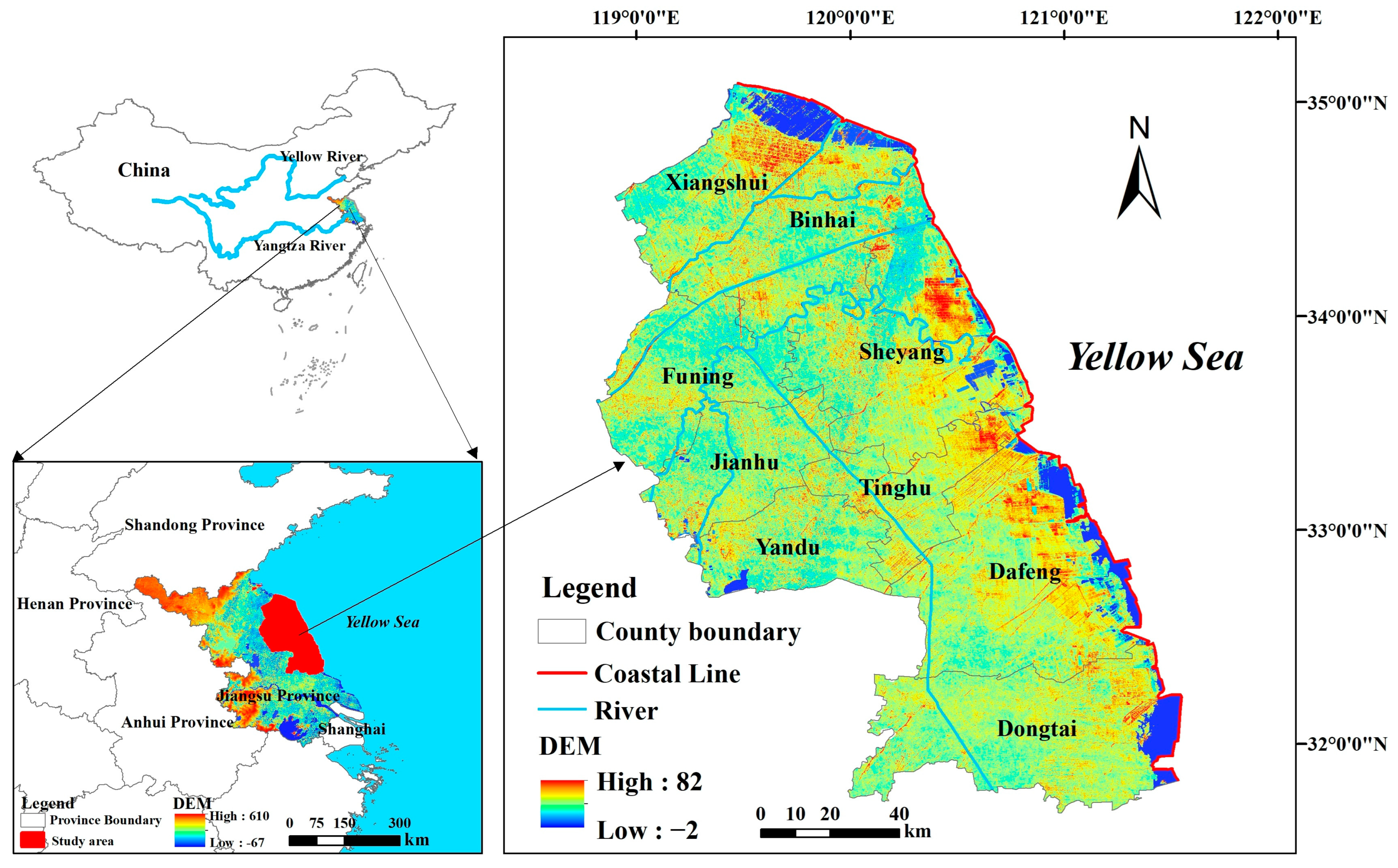
2.1. Study Area

Yancheng is situated on the shores of the Yellow Sea and the eastern coast of China, between 32°34′ N~34°28′ N and 119°27′ E~120°54′ E (Figure 1), being one of the cities at the center of the Yangtze River Delta. Its scope includes three districts, namely, Tinghu, Yandu, and Dafeng; five counties, namely Jianhu, Sheyang, Funing, Binhai, and Xiangshui; and one county-level city, Dongtai. The total land area is approximately 17,718 km², among which the coastal area is 4553 km², accounting for 70% of the mudflat region of Jiangsu Province. The coastline is 582 km long, taking up 56% of Jiangsu province’s total coastline length. Located at the crossroads of land and sea, Yancheng is home to the biggest coastal wetland on the west coast of the Pacific Ocean and the edge of the Asian continent and was named a World Natural Heritage Site in 2019, known as the “Wetland Capital of the East”. Yancheng is located in the transition zone from the northern subtropical zone to the warm temperate zone, with superior water and heat conditions, flat terrain, and a dense water network. Its climate is strongly influenced by the ocean, with a distinct monsoon climate.

2.2. Data Source and Preprocessing

The land use data of Yancheng were derived from Landsat TM images of 30 m × 30 m resolution for five periods in 2000, 2005, 2010, 2015, and 2020 from the Resource and Environment Science Data Center of the Chinese Academy of Sciences (https://www.resdc.cn, accessed on 1 December 2022). The data of six land use types in the study area, i.e., farmland (Fal), forest land (Fol), grassland (Grl), construction land (Col), water body (Wat), and unused land (Unl), were obtained through human-computer interaction interpretation, and the classification accuracy reached more than 94% after the accuracy test to satisfy the research needs [34]. The data on grain yield, unit price, and sown area used to compute ESV per unit area were sourced from the Jiangsu Statistical Yearbook and the China Agricultural Price Survey Yearbook for the corresponding years.

The selection of factor indicators took into account climate, topography, socio-economics, and land use that may influence changes in ecosystem function. Specific to the actual area of study, six indicators that were more commonly cited were ultimately selected based on climatic, topographic, socio-economic, and land-use factors [7,35], including (1) climate factors, such as average annual temperature (TEM), average annual rainfall (RAI); (2) topography factors, such as average elevation (DEM); (3) socio-economic factors, such as population density (POP) and economic density (GDP); (4) land use factors, such as land development intensity (LDI). Among them, the average elevation data were extracted through the geospatial data cloud, the land development intensity was calculated by referring to the formula proposed by Brentrup et al. (2002) (for more details, see He et al., 2021 [36]), and the remaining data were collected by visiting the Data Centre for Resource and Environmental Sciences of the Chinese Academy of Sciences.

2.3. Study Methods

2.3.1. Measurement of the ESV

The equivalent factor method is widely employed for estimating ESV at a wide range of geographic scales due to its relatively small amount of data required and rapid assessment [31]; hence, it is chosen for this paper. Xie et al. adapted the equivalent factor method proposed by Costanza et al. to the context of China, which reflected the characteristics of ecosystem services in China [37]. Considering the higher number and return rate of questionnaires based on its 2008 research results [12], which were more scientific and credible, we adopted it as the national base value equivalent factor scale. By consulting the Jiangsu Statistical Yearbook and the China Agricultural Products Price Survey Yearbook, the average yield value of major crops was calculated by using the average production (6721.13 kg·hm⁻²) and average price (2.23 yuan·kg⁻¹) of major crops in the study area in the five years of 2000, 2005, 2010, 2015 and 2020, and finally obtaining the value of the study area’s 1 standard equivalent corrected value of 2145.08 yuan·hm⁻².

Considering that the ecosystem of the study area is constantly changing in space and time, and the ESV changes dynamically accordingly, we introduced a functional adjustment factor to dynamically adjust the equivalence factor based on the situation of the study area. In this paper, the ratio of unit grain production in the study area to the national average was taken as the functional adjustment coefficient for supply services, and the ratio of NPP in the study area to the national average NPP was taken as the functional adjustment coefficient for regulation and support services, to construct a spatiotemporal dynamic value equivalent table for ESV [38]. The formula is as follows.

$$V{C}_{kjt}=S_{kj}\times F_{jt}$$

(1)

where $V{C}_{kjt}$ is the equivalent factor of the $j$-th ecological service function of the $k$-th land type in $t$ year (yuan·hm⁻²·a⁻¹); $S_{kj}$ is the national equivalence factor for the $j$-th ecosystem service function of the $k$-th land type (yuan·hm⁻²·a⁻¹); $F_{jt}$ is the adjustment coefficient for the $j$-th ecosystem service function in year $t$.

The ESV for each study unit was then calculated based on the area of the different land types, resulting in a total ESV for the study area.

$$ES{V}_{it}={\displaystyle \sum _{k=1}^l{\displaystyle \sum _{j=1}^m{A}_{ikt}\times V{C}_{kjt}}}$$

(2)

$$AES{V}_{it}=\frac{ES{V}_{it}}{A_{it}}$$

(3)

$$TES{V}_t={\displaystyle \sum _{i=1}^{n}ES{V}_{it}}$$

(4)

where $ES{V}_{it}$ indicates the $ESV$ of the $i$-th study unit in year $t$ (yuan). $AES{V}_{it}$ indicates the $ESV$ of the unit area of the $i$-th study unit in year $t$ (yuan·hm⁻²). $A_{it}$ indicates the area of the $i$-th study unit in year $t$ (hm²). $TES{V}_t$ indicates the total ESV in the study area in year $t$ (yuan). $A_{ikt}$ indicates the area of the $k$-th land type in the $i$-th study unit in year $t$ (hm²). $i$, $j$, $k$ indicate the study unit number, ecosystem service function, and land use type in order.

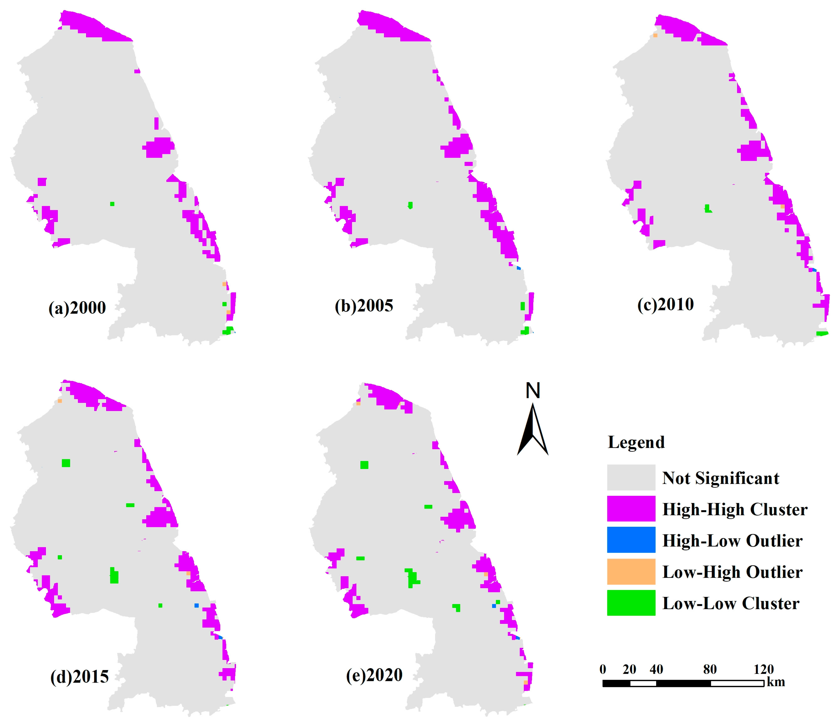
2.3.2. Spatial Autocorrelation Analysis

(1)

Global Moran’s I

To further investigate the heterogeneity of the spatial distribution of ESV in Yancheng, the global Moran’s I was introduced as an indicator for the correlation and degree of difference among the spatially adjacent or similar regional unit observations across the study area. The calculation formula is as follows.

$$I_G=\frac{1}{S^2{\displaystyle \sum _{k=1}^n{\displaystyle \sum _{l=1}^n{\omega }_{kl}}}}{\displaystyle \sum _{k=1}^n{\displaystyle \sum _{l=1}^n{\omega }_{kl}}}(x_k-\overline{x})(x_l-\overline{x})$$

(5)

where $x_k$ and $x_l$ represent the observed values of the study unit $k$ and $l$, respectively. $\overline{x}$ represents the observed mean value. ${\omega }_{kl}$ represents the spatial weight, with 1 for spatial adjacency and 0 for non-adjacency.

(2)

Local Moran’s I

The local Moran’s I is a common index to gauge the extent of spatial autocorrelation between a regional unit and its neighboring regional units, which can further reflect the local spatial variation features of ESV in Yancheng. The calculation formula is as follows.

$$I_k=z_k^t{\displaystyle \sum _{t=1}^n{\omega }_{kl}}{z}_l^t$$

(6)

where $z_k^t$ and $z_l^t$ represent the normalization of the study unit $k$ and $l$ observations, respectively. ${\omega }_{kl}$ represents the spatial weight, with ${\displaystyle \sum _{t=1}^n{\omega }_{kl}=1}$.

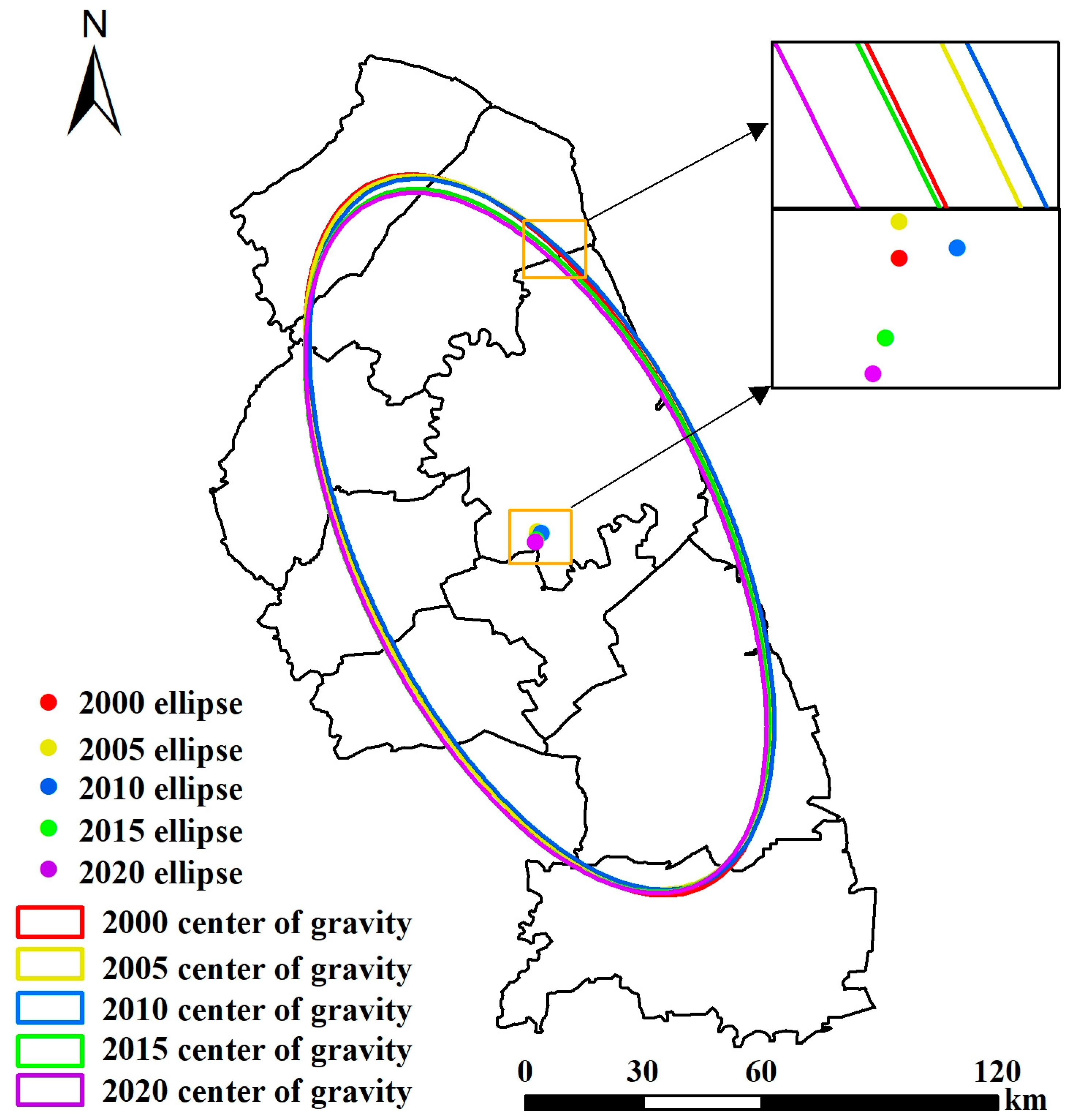
2.3.3. Standard Deviation Ellipse

The standard deviation ellipse can measure the spatial distribution trend of spatial attribute data, and its elements include the rotation angle $\theta$, the standard deviation value along the x-axis, and the standard deviation value along the y-axis [7]. The long y-axis denotes the distribution orientation of the spatial attribute data, the short x-axis indicates the distribution range of the spatial attribute data, and the flatness of the standard deviation ellipse indicates the degree of spatial distribution directionality. The Equations for each basic parameter are as follows.

$$\overline{X_{\omega }}=\raisebox{1ex}{${\displaystyle \sum _{i=1}^n{\omega }_i{x}_i}$}\!\left/ \!\raisebox{-1ex}{${\displaystyle \sum _{i=1}^n{\omega }_i}$}\right.,\overline{Y_{\omega }}=\raisebox{1ex}{${\displaystyle \sum _{i=1}^n{\omega }_i{y}_i}$}\!\left/ \!\raisebox{-1ex}{${\displaystyle \sum _{i=1}^n{\omega }_i}$}\right.$$

(7)

$$\tan \theta =\frac{{\displaystyle \sum _{i=1}^n{\omega }_i{}^2{\tilde{x}}_i{}^2}-{\displaystyle \sum _{i=1}^n{\omega }_i{}^2}{\tilde{y}}_i{}^2+\sqrt{{\left({\displaystyle \sum _{i=1}^n{\omega }_i{}^2{\tilde{x}}_i^2}-{\displaystyle \sum _{i=1}^n{\tilde{y}}_i^2}\right)}^2+4{\displaystyle \sum _{}^{}{\omega }_i{}^2{\tilde{x}}_i^2{\tilde{y}}_i^2}}}{2{\displaystyle \sum _{i=1}^n{\omega }_i{}^2{\tilde{x}}_i{\tilde{y}}_i}}$$

(8)

$${\sigma }_x=\sqrt{{\displaystyle \sum _{i=1}^n{({\omega }_i{\tilde{x}}_i\cos \theta -{\omega }_i{\tilde{y}}_i\sin \theta )}^2}/{\displaystyle \sum _{i=1}^n{\omega }_i{}^2}}$$

(9)

$${\sigma }_y=\sqrt{{\displaystyle \sum _{i=1}^n{({\omega }_i{\tilde{x}}_i\sin \theta -{\omega }_i{\tilde{y}}_i\cos \theta )}^2}/{\displaystyle \sum _{i=1}^n{\omega }_i{}^2}}$$

(10)

where $({\overline{X}}_{\omega },{\overline{Y}}_{\omega })$ denotes the weighted mean center of the spatial dataset of the study subject; ${\omega }_i$ denotes the weight; $(x_i,y_i)$ denotes the spatial coordinates of the study object; $\sigma$ denotes the azimuth of the ellipse; $\widetilde{x_i}$ and ${\tilde{y}}_i$ denote the deviation of the study object′s spatial coordinates from the mean center, respectively. ${\sigma }_x$ and ${\sigma }_y$ denote the standard deviation of the x-axis and y-axis, respectively.

2.3.4. Driving Force Analysis Method

GeoDetector makes up for the shortcomings of the lack of spatial differentiation studies and the limitations of assumption conditions in traditional statistics and combines ArcGIS spatial overlay technology and set theory to effectively identify synergistic or antagonistic relationships between multiple factors [39]. GeoDetector reveals the reasons behind spatially stratified heterogeneity without the need for linearity assumptions and effectively identifies explanatory variables that have a significant effect on the dependent variable, which is widely used in the fields of land use, regional planning, and ecological environment [31,40,41]. The GeoDetector model consists of four basic models: risk, factor, ecological, and interaction detectors [42]. In contrast to traditional measures, factor detection can measure the power of individual factors driving regional ESV spatial variation by q-values, and interaction factor detection can further identify the interactive effects of different factors on regional ESV spatial variation. In this study, we mainly employed the factor detector and interaction detector in the GeoDetector to explore the drivers of the spatial differentiation of ESV in Yancheng. The expression of the model is as follows.

$$q=1-\frac{1}{N{\sigma }^2}{\displaystyle \sum _{h=1}^L{N}_h{\sigma }_h{}^2}$$

(11)

where $q$ is the explanatory power of the influencing factors on the spatially divergent features of ESV, and its value ranges from 0 to 1. The higher the value, the stronger the explanation of the independent variable X on the dependent variable Y, and vice versa. $L$ is the number of classifications or partitions of ESV spatial differentiation influences X. $N_h$ and $N$ are the number of samples in stratum $h$ and study area, respectively.${\sigma }_h{}^2$ and ${\sigma }^2$ are the variance of ESV in layer $h$ and study area, respectively.

3. Results

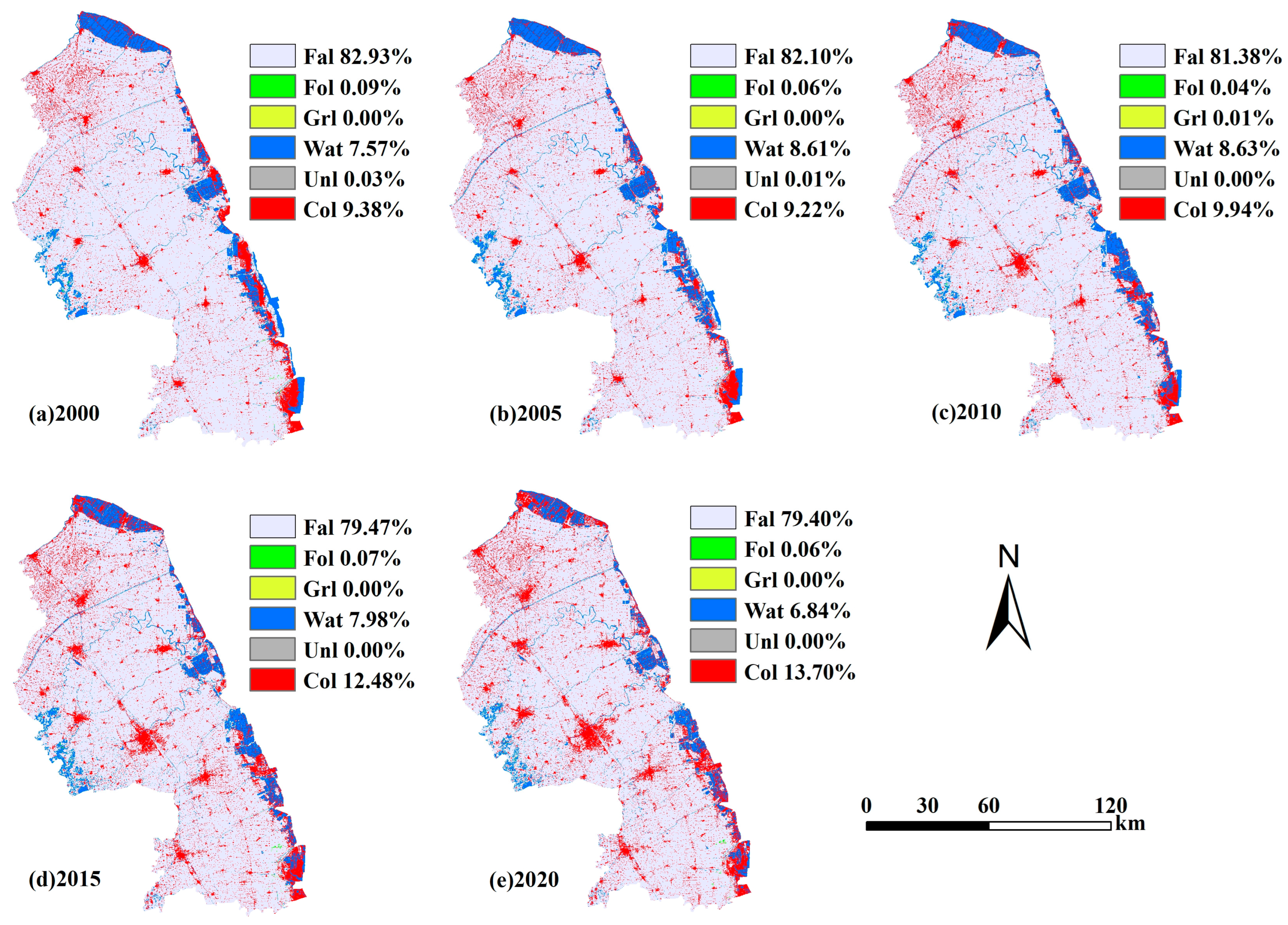
3.1. Land Use Change Characteristics

As can be seen from Figure 2, land use types in the study area during 2000–2020 were dominated by farmland, making up over 79% of the total area, followed by construction land and water bodies, making up over 9.3% and 6.8%, respectively. The area of other land use types was quite small, totaling less than 1.5%. Due to the effects of human production and life, the construction land area continued to increase, while the areas of other land types were reduced to varying degrees. The area of construction land expanded year by year, showing a radial structure centered on the county and along the main transport routes, with the largest increase of 46% and a cumulative increase of 962.69 km², from 9.38% in 2000 to 13.70% in 2020. The area of farmland declined gradually from 18437.46 km² (82.92%) in 2000 to 17653.36 km² (79.4%), with a decrease of 784.10 km². The water body area showed a tendency to increase and then decrease, with the percentage increasing from 7.57% in 2000 to 8.63% in 2010 and then gradually decreasing to 6.84% in 2020.

Table 1. Land use transfer in the study area from 2000 to 2020.

Year	Type	Items	2020
			Fal	Fol	Grl	Wat	Unl	Col	Transfer Out
2000	Fal	Area/km2	12,709.40	4.36	0.03	264.35	0.03	697.98	966.75
		Transfer out rate/%		0.451	0.003	27.344	0.003	72.199	100.000
	Fol	Area/km2	8.20	5.18	0.00	1.37	0.00	0.40	9.97
		Transfer out rate/%	82.247		0.000	13.741	0.000	4.012	100.000
	Grl	Area/km2	0.47	0.00	0.02	0.16	0.00	0.15	0.77
		Transfer out rate/%	60.256	0.000		20.513	0.000	19.231	100.000
	Wat	Area/km2	311.16	0.19	0.00	697.77	0.08	240.79	552.22
		Transfer out rate/%	56.347	0.034	0.000		0.014	43.604	100.000
	Unl	Area/km2	1.56	0.00	0.00	2.21	0.15	1.49	5.27
		Transfer out rate/%	29.658	0.000	0.000	42.015		28.327	100.000
	Col	Area/km2	63.91	0.00	0.00	162.80	0.01	1319.50	226.72
		Transfer out rate/%	28.189	0.000	0.000	71.807	0.004		100.000

Notes: Definitions of acronyms are given in Figure 2.

presents a complex transfer that occurred between all land use types in Yancheng from 2000 to 2020, with a total transfer area of 1761.7 km². Farmland contributed the most to the transferred area with 966.75 km², of which 697.98 km² changed to construction land, accounting for 72.199%, and 264.35 km² changed to water body, accounting for 27.344%. The second largest transfer out was from water bodies, with 552.22 km², of which 56.347% was transformed into farmland and 43.604% into construction land. The third largest amount of construction land was transferred out, 226.72 km², of which 162.8 km² (71.807%) turned into water bodies and 63.91 km² (28.189%) turned into farmland. The majority of the transfer out from other land use types became farmland. Construction land was the most imported land type, with 940.81 km², followed by water bodies and farmland, with 430.89 km² and 413.44 km², respectively. The reason for this phenomenon was that the fast-growing economy entailed the massive occupation of farmland on the outskirts of towns and cities, while the use of other ecological land was changed to ensure food security and strict adherence to the red-line policy for farmland. In addition, the execution of ecological conservation engineering and settlement improvement has brought about a more complex and diverse land conversion.

3.2. ESV Change Characteristics

3.2.1. ESV Temporal Change Characteristics

Over the period 2000 to 2020, the total ESV in the study area exhibited a pattern of increasing and then decreasing, rising from 547.84 × 10⁸ yuan in 2000 to 570.79 × 10⁸ yuan in 2005 and gradually decreasing thereafter to 507.62 × 10⁸ yuan in 2020, with a total decrease of 40.22 × 10⁸ yuan, a change rate of −7.34% (Figure 3). In terms of the percentage of ESV for each land type, the ranking from largest to smallest was as follows: farmland > water body > forest land > grassland > unused land. Among them, the total value of farmland and water bodies exceeded 99%, in an overwhelmingly dominant position, while the total value of other land types was a smaller percentage, less than 1%. ESV in farmland experienced a continuous reduction at a change rate of 5.76%, while ESV in water bodies trended towards an increase followed by a decrease, similar to total ESV, at a change rate of −10.11% (

Table 2. ESV of different land use types in Yancheng from 2000 to 2020.

Land Use type		Fal	Fol	Grl	Wat	Unl
ESV (108 yuan)	2000	357.81	1.43	0.03	188.54	0.02
	2005	354.19	0.87	0.02	215.77	0.01
	2010	351.53	0.77	0.05	215.14	0.00
	2015	340.22	1.09	0.01	195.44	0.00
	2020	337.21	0.93	0.00	169.47	0.00
Changes rate (%)	2000–2005	−1.01	−39.07	−37.96	14.44	−73.01
	2005–2010	−0.75	−11.89	166.35	−0.29	−51.42
	2010–2015	−3.13	40.98	−71.67	−9.16	−36.95
	2015–2020	−0.98	−14.23	−86.21	−13.29	−42.16
	2000–2020	−5.76	−35.09	−93.55	−10.11	−95.22

Notes: The definitions of acronyms are given in Figure 2.

). The rate of change in ESV was greater for the other land types, but the impact on total ESV was weak due to their small absolute values. For example, while the rate of change in ESV for grassland between 2005 and 2010 was 166.35%, its value increased by just less than 3 million yuan. The same was true for the change in ESV for forest land. Therefore, changes in ESV for Yancheng were primarily attributable to the alteration in the land type of farmland and water bodies.

From the primary classification, regulation services, and support services contributed the most to the total ESV. From 2000 to 2020, the value of all four functional services trended upwards and then downwards, achieving a maximum value in 2005 and a minimum value in 2020 (Figure 3). The four service values decreased by 8.17% (supply services), 7.05% (regulation services), 5.24% (support services), and 8.22% (cultural services), respectively. In terms of the secondary classification, the WT function had the highest value, contributing the most to the total ESV at 23.01%~23.68%, followed by the HR function at 20.59%~22.06%. In contrast, the lowest contribution was the RMS function, with only 3.47%~3.92% (

Table 3. Changes in the value of individual ecosystem services in the study area from 2000 to 2020.

Subtype	2000	2005	2010	2015	2020	2000–2020
						Change Rate (%)
FS	42.01 (7.67)	46.69 (8.12)	41.54 (7.32)	40.35 (7.56)	39.87 (7.81)	−5.10
RMS	21.45 (3.92)	19.96 (3.47)	20.69 (3.65)	19.54 (3.66)	18.41 (3.61)	−14.18
GR	35.54 (6.49)	35.55 (6.18)	35.19 (6.20)	33.63 (6.30)	33.75 (6.61)	−5.03
CR	53.56 (9.78)	54.43 (9.47)	53.96 (9.51)	51.22 (9.60)	50.61 (9.91)	−5.51
HR	114.60 (20.92)	125.52 (21.84)	125.20 (22.06)	115.38 (21.62)	105.13 (20.59)	−8.26
WT	126.54 (23.10)	135.00 (23.49)	134.40 (23.68)	125.10 (23.44)	117.48 (23.01)	−7.16
SC	69.63 (12.71)	69.39 (12.07)	68.78 (12.12)	65.72 (12.31)	66.35 (12.99)	−4.71
MB	61.64 (11.25)	63.31 (11.01)	62.82 (11.07)	59.38 (11.12)	58.04 (11.37)	−5.84
EAC	22.86 (4.17)	24.95 (4.34)	24.92 (4.39)	23.42 (4.39)	20.98 (4.11)	−8.22

Note: The unit of ESV is 10⁸ yuan. The numbers in parentheses are the proportions. Food supply (FS), Raw material supply (RMS), Gas regulation (GR), Climate regulation (CR), Hydrological regulation (HR), Waste treatment (WT), Soil conservation (SC), Maintaining biodiversity (MB), Entertainment and culture (EAC).

). Between 2000 and 2020, the value of each secondary ecosystem service function generally trended downwards overall, among which the values of RMS, GR, and SC functions showed a descending tendency annually, with change rates of −14.18%, −5.03%, and −4.71%, respectively. The values of FP, CR, HR, and WT functions showed an upward and then downward trend, while the value of the EAC function showed a decrease of 8.22%.

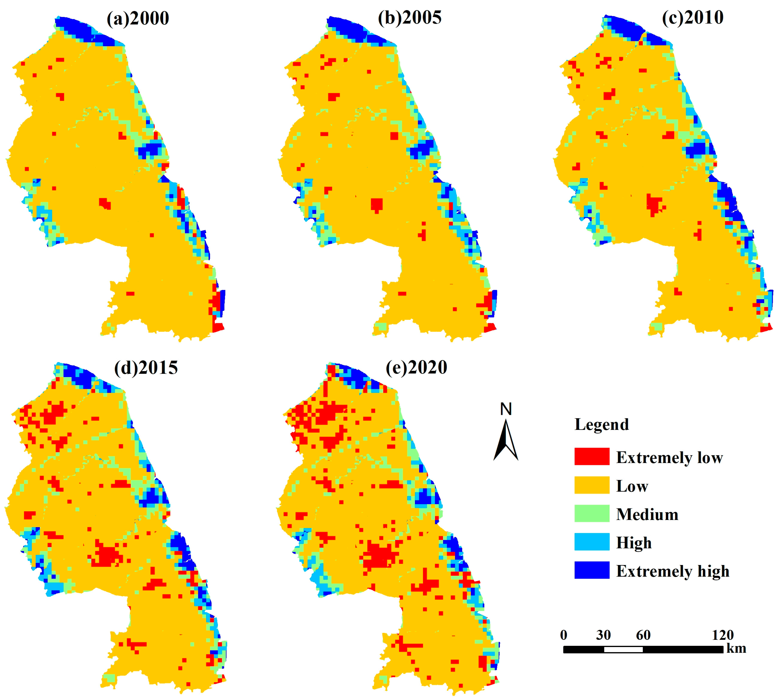
3.2.2. ESV Spatial Change Characteristics

To elucidate the characteristics of the spatial differentiation of ESV in the study area, it was required to select the suitable scale as the study unit. After reviewing the relevant literature, we found that the smallest scale used for this kind of study was 1 km × 1 km grid, which could reflect the spatial and temporal heterogeneity of ESVs well, but it was difficult to generalize the results to a wide range of ecological conditions because of the small scale. Therefore, considering the ease of data processing and the applicability of the results, this paper selected the 3 km × 3 km grid, which was adopted by many scholars [7,43]. As can be seen in Figure 4, there were significant differences in the spatial distribution of ESV in the study area at the three scales, with the finest spatial distribution of ESV at the grid scale, followed by the township scale, and finally, the county scale. The smaller the study unit at the grid scale, the original differentiation information would be retained, and the evaluation results would be more accurate, and the opposite was true at the large scale. Meanwhile, we applied the global spatial autocorrelation test and found that only the grid scale passed the test of significance at the 1% level, while both the township scale and the county scale failed, indicating that the grid scale was the most appropriate. Thus, this paper chose the research unit scale of 3 km × 3 km for investigating the spatiotemporal differentiation characteristics and driving mechanism of ESV in the study area.

In this paper, by calculating a unit area ESV (yuan·hm⁻²) of the evaluation cells of 3 km × 3 km, combining the central assignment method with ArcGIS software for the spatial assignment. The natural interruption point grading method was used to classify the ESV of the evaluation unit in the study area into five categories, namely very low, low, medium, high, and very high, which was adopted by many scholars [44,45], and finally formed the spatial pattern distribution map of ESV in the five periods (Figure 5). As can be seen from Figure 5, the overall distribution of ESV in Yancheng during the 21 years showed a marked variability with higher characteristics in the eastern coastal region than in other regions. The ESV was higher in the eastern area along the Yellow Sea, with high and extremely high grades predominating, and the main urban areas of the county (district and city) were concentrated with extremely low grades. The study area was overwhelmed by low ESV, with a gradually decreasing area share, averaging 75.87%, which was consistent with the spatial distribution characteristics of the farmland. The proportion of extremely low-grade areas gradually increased, from 2.56% in 2000 to 7.08% in 2020, an increase of 4.52%. It was mainly transformed from low-grade and concentrated in the distribution of construction land with active human activities. The extremely high-grade area was on a shrinking trend, decreasing from the initial 4.53% to 3.35%, especially after 2010, with the implementation of Jiangsu’s coastal development strategy, decreasing by as much as 1.63%. The proportion of medium and high grades tended to rise and then fall.

To investigate the spatial clustering features of ESV in Yancheng, the GeoDa software was utilized to calculate the global Moran′s I for ESV at a 3 km × 3 km grid scale. The results of the autocorrelation analysis in

Table 4. Global spatial autocorrelation of ESV.

Index	2000	2005	2010	2015	2020
Global Moran’s I	0.6646	0.6918	0.6589	0.6324	0.6169
Z-score	50.2452	52.2817	49.7993	47.7979	46.7941
p-value	0.0000	0.0000	0.0000	0.0000	0.0000

showed that Moran’s I was greater than 0 in all five periods with a p-value of 0 at a 99% confidence level and Z-score minimized at 46.7941 which indicated positive spatial autocorrelation of ESV in the study area. Moran’s I peaked at 0.6918 in 2005 and trended downwards around 2005 to a minimum of 0.6169 in 2020. From Figure 6, it can be seen that the high–high ESV aggregation areas were primarily spread along the eastern coastal zone and in the western Sheyang River along Yandu District and Jianhu County, and the number of aggregated grids fluctuated over time. The low-low aggregation areas were sporadically scattered in the town centers, and their grid numbers incrementally increased over time. Most other grids were not significant.

We employed ArcGIS 10.2 software to plot standard deviation ellipses for the gravity center position to investigate the typical characteristics of ESVs as well as the states and directions of displacements occurring in the time series. As can be seen from Figure 7, from 2000 to 2020, the gravity center of ESV distribution in all years was located in the southwestern part of Sheyang County, moving roughly along the north-northeast–southwest direction from Sheyang County to the junction of Tinghu District in the southwestern direction. The changes of long and short axis lengths showed opposite trends, with the long axis length decreasing and the short axis length increasing, suggesting a centripetal clustering of ESV in the northwest-southeast direction and a spatially dispersed trend in the northeast–southwest direction in the study area. Azimuth presented a fluctuating trend, but the variation was small, demonstrating that the direction of ESV distribution dispersion in the study area was comparatively stable.

3.3. Driving Force of Spatial Heterogeneity in ESV

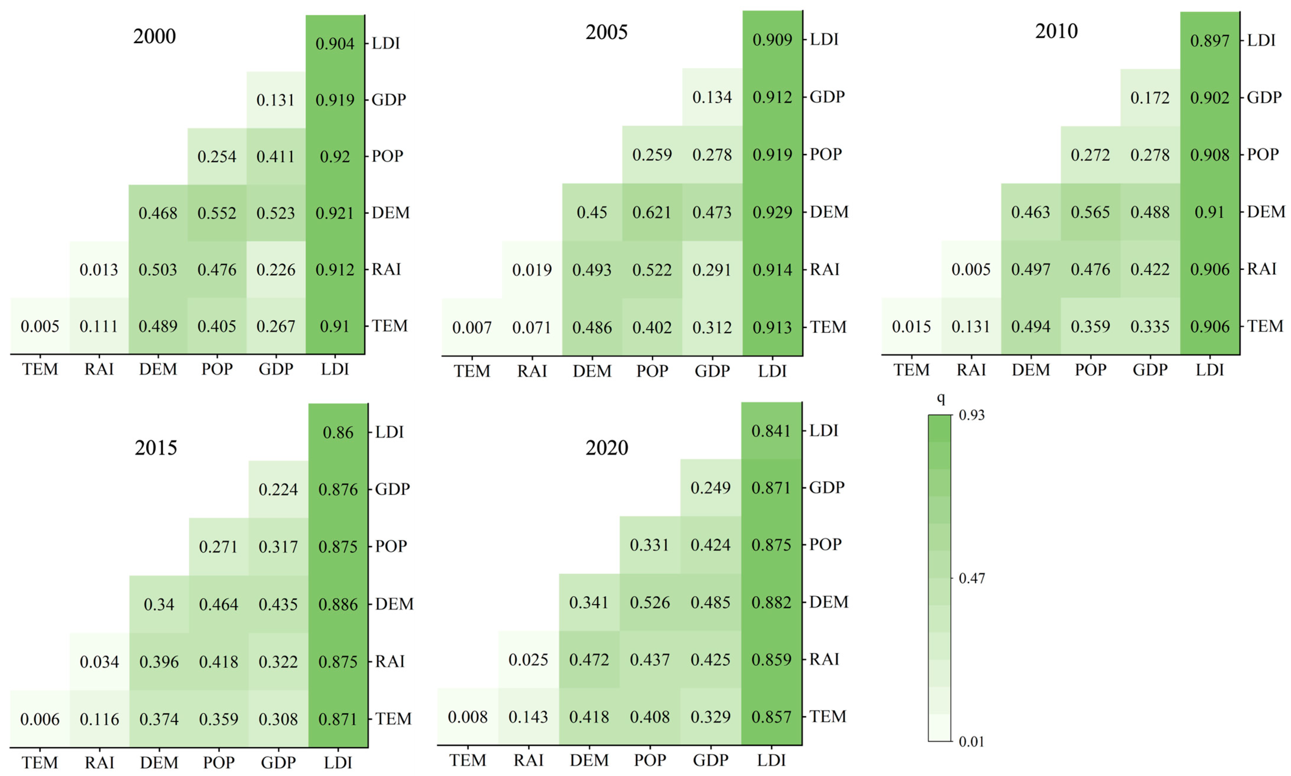
3.3.1. Factor Probe Analysis

For accurate model estimation, we first employed the variance inflation factor to test for multicollinearity among the drivers. The results showed that the variance inflation factor values of the seven drivers are less than 10, and there was no serious multicollinearity among the variables. Based on a comprehensive comparison of various methods, we adopted the natural interruption point grading method as a statistical method to classify similar values according to numerical laws, which can appropriately group the similar values to maximize the differences between the groups [7], and used the ArcGIS software to classify each driving factor into different grades. GeoDetector was applied to calculate and get the detection results of the factors affecting the ESV radiation dispersion in Yancheng in different periods. As shown in

Table 5. The contributions (q statistics) of driving factors to ESV variation.

Driving Factor	2000		2005		2010		2015		2020
	q Statistic	p Value	q Statistic	p Value	q Statistic	p Value	q Statistic	p Value	q Statistic	p Value
TEM	0.005	0.012	0.007	0.000	0.015	0.000	0.006	0.003	0.008	0.000
RAI	0.013	0.000	0.019	0.000	0.005	0.032	0.034	0.000	0.025	0.000
DEM	0.468	0.000	0.450	0.000	0.463	0.000	0.340	0.000	0.341	0.000
POP	0.254	0.000	0.259	0.000	0.272	0.000	0.271	0.000	0.331	0.000
GDP	0.131	0.000	0.134	0.000	0.172	0.000	0.224	0.000	0.249	0.000
LDI	0.904	0.000	0.909	0.000	0.897	0.000	0.860	0.000	0.841	0.000

Notes: The q value indicates the magnitude of the driving force.

, all factors passed the significance test at the 5% level, indicating that they all significantly drove the distribution of ESV. Overall, the explanatory power of the drivers varied across time, but the ranking was always in the order of LDI > DEM > POP > GDP > RAI > TEM. Factors such as LDI and DEM laid the foundation of the spatial distribution of ESVs in the study area and controlled the disturbance of the ecological environment by human activities, especially the spatial difference of LDI significantly influenced the spatial pattern of ESVs.

Between 2000 and 2020, the q-value of LDI exhibited a general downward trend, decreasing from 0.904 in 2000 to 0.841 in 2020, indicating that the impact of the continuously optimized land development and utilization patterns on ecosystem services has gradually become smaller in recent years. The explanatory power of the topography factor DEM (0.468~0.341), although weakened, was still above 40%. It was worth noting that the q-values of socio-economic factors POP (0.254 to 0.331) and GDP (0.131 to 0.249) continued to increase, which indicated the enhanced influence of human life production activities on the distribution of ESVs. Special attention should be paid to harmonizing socio-economic development and ecological protection in future coastal development. The q-values of the climatic factors TEM and RAI changed in different periods, but their explanatory power was relatively weak.

3.3.2. Interaction Probe Analysis

The interaction detection analysis was a major advantage of the GeoDetector tool, which could reflect the results of the action on the ESV distribution under the two-factor effect, as shown in Figure 8. The explanatory forces of the individual factors were all smaller than those following the interactions between the factors, and the interactions between the factors all tended to be non-linearly enhanced and bi-factorially enhanced. The interactions of LDI with the other drivers had more than 80% explanatory power at different times, with the largest q-value for the interaction with DEM. This was followed by a significant interaction enhancement effect of DEM with POP, all of which had more than 50% explanatory power. During the period 2000–2020, GDP and POP had a weak explanatory power under the analysis of single-factor effects, but the interactions with the factors LDI and DEM, which had the highest single-factor effects, were significantly enhanced under the interaction factors, and their interactive explanatory powers were all above 40%. While single socio-economic factors had a limited impact on ESV distribution, the role of land use and topographic factors significantly increased their impact, especially in flat and resource-rich coastal areas, as evidenced by the rapid concentration of population in coastal areas. Overall, the ESV differentiation was jointly influenced by multiple drivers, with each factor showing an isotropic interaction of varying strengths, and all of the interactions were larger than the effects when acting alone.

4. Discussion

4.1. Land Use and ESV Change Analysis

Over the past 21 years, the land landscape pattern in the study area has changed significantly, with a large number of beaches and water bodies in the coastal zone being transformed into construction land or artificial ponds and farmland being continuously encroached upon, resulting in an obvious contradiction between people and land, which is basically in line with the findings of related scholars [27,32]. The anthropogenic nature of the land conversion process in Yancheng became more obvious, and the disturbance and destruction of the land surface by human activities intensified, especially the reduction of arable land and water area posed a threat to regional food security and biodiversity [46]. In recent years, the implementation of the policy of strictly adhering to the red line of arable land has eased the rate of arable land decline, which should continue to be strengthened in the future. As the coastal development and urbanization of Jiangsu Province accelerated in 2009, the watershed area of Yancheng continued to decline due to gradual erosion [47], and the decline gradually increased, with a decline of up to 14% from 2015 to 2020, while more patches of construction land appeared. This is consistent with the trend of the findings of Bao, et al., 2019 [48].

Most of the existing studies related to the spatio-temporal differentiation of ESV use administrative divisions as the unit of study, but they are unable to express the differences within the administrative division units. In this study, the size of the grid cell was determined based on the size of the integrated landmarks and the area of the study area to better reveal the spatial and temporal differentiation characteristics of ESV in the study area, and the results of the study were the same as those of the previous researchers [32,49]. Yancheng, being a coastal city, has abundant hydrothermal conditions that form a large amount of vegetation biomass. Therefore, the ESV calculated based on the corrected ESV dynamic equivalent table was more accurate. From 2000 to 2020, the ESV in the study area trended up and then down, with an overall decrease (Figure 3). In the early stage, the Yancheng economy had not yet been fully launched when the local ecology was less disrupted. After 2005, with the increasing scale of undertaking the industrial transfer from southern Jiangsu, the overall regional economy developed rapidly, and high ESV coefficient land types were appropriated by low ESV coefficient land types [49]. Land use and land cover changes have altered ecosystem architecture and function, such as loss of arable land, degradation of wetlands, and significant growth in the area of built-up land, resulting in a deterioration of regional ecological quality [18,50]. The ESV coefficients of forests and water bodies were notably higher than those of farmland [51]; however, the area base of farmland was considerably greater in comparison to them, and even though its area was decreasing during the study period, it still contributed the most to ESV. Forest land contributed less than 3% to ESV due to its small absolute area, but its change rate was large. In particular, the change rate of 2010–2015 was 40.98%, which is closely related to the policy of returning farmland to forests implemented in the same period.

Coastal areas usually have highly developed economies due to abundant water resources and suitable environments, which drive frequent land use changes, especially the phenomenon of land urbanization [52,53]. The continuous expansion of built-up land under direct human intervention was at the sacrifice of ecological land [31], and its contribution to ESV was lower than that of other land types, which would reduce regional ESV [28,54]. Among the primary ESV functional classifications, regulation services made the greatest contribution and performed a vital action on ESV changes, which was largely in line with the trend of ESV changes in coastal areas [11,55,56]. In the secondary ESV function classification, waste treatment and hydrological regulation represented the biggest portion of the total ESV at approximately 43%, further evidence of the high dependence of ecosystem health on hydrological conditions in Yancheng [57]. The execution of ecological restoration projects in the area, such as returning farming and fishing to wetlands, has a positive significance in restraining the unreasonable exploitation of land resources.

4.2. Driving Factors on ESV Distribution

Studying the extrinsic spatial and temporal evolution and intrinsic driving mechanisms of ESV can provide an important basis for identifying ecosystem service problems in coastal areas, maintaining regional ecological balance, and promoting regional sustainable development [58]. The results of factor detection indicated that land use was the most important driver of ESV, which was consistent with other scholars′ studies [32,59]. Natural ecosystems were land-based, and land use intensity determined the degree of conversion of ecological land to artificial land. DEM showed better explanatory power for the spatial differentiation of ESV. The differences in DEM altered the regional ecology, affecting the extent of human activities, especially in the lower elevation plains of the coastal zone where human intervention was higher and ESV was lower [60]. The explanatory power of socio-economic factors on ESV in this study gradually increased over time, indicating that with the deepening of coastal development policies in Jiangsu, the intensity of human activities increased, and especially coastal population agglomerations became more influential on ESV [61]. We found that the relatively weak explanatory power of climatic factors on ESV may be due to the study area being dominated by farmland ecosystems, and the ESV of small-scale farmland was not sensitive to climatic factors, coupled with the selection of smaller grid cell further weakened the influence of climatic factors on it [62].

ESV spatial differentiation was the result of multiple factors driving together, so the single-factor detection results could not scientifically reveal the contribution of synergistic effects among factors [63]. Factor interactions had a greater influence on the spatial distribution of ESV, and there was a coupled relationship between land use, topography, socio-economic and climate factors. Land use created the basic pattern of regional ESV differentiation, and the explanatory power of interaction with topography factors was significantly increased. Land use practices changed the distribution of habitats and resources [64], especially the fragmentation of land patches affects the connectivity of ecological landscapes deteriorates, leading to a decrease in the regulatory capacity of ecosystems and inhibiting the ESV on enhancement [65]. Socio-economic factors had an increased influence on ESV through the role of land use, meteorology, and topography, suggesting that economic development may change the direction of ecosystem service evolution in the process of natural change, which was consistent with the findings of Liu, et al., 2019 [66]. The direct effects of the climate factors TEM and RAI on ESV were weak, but their explanatory power increased after interaction with other factors. Climate change affects coastal ecosystems depending on changes in the natural environment and related ecological attributes [14]. Therefore, in the practice of ecosystem optimization and ecological risk management in Yancheng, it is necessary to take into account the specificity of the various factors and the synergistic enhancement effect of each factor and implement diverse multi-regulation approaches [45,67].

It was essential to choose land use development patterns that were appropriate to the region’s natural contexts and degree of socio-economic growth to avoid unreasonable or strong anthropogenic land use disturbances [68]. Yancheng, as a largely agricultural city, should focus on strengthening the construction of ecological agriculture and weakening the negative impact of arable land on the ecological environment. In economically developed regions, the negative impact of socio-economic development on the natural ecological environment can be weakened through measures such as optimizing the layout of land use and enhancing the connectivity of water systems. Meanwhile, it is necessary to strengthen the protection of wetlands, further carry out the project of returning fisheries to wetlands in a scientific manner and construct small and micro-wetlands relying on estuaries and salt flats to give full play to the ecological functions of the waters.

4.3. Limitations and Future Work

The analysis of the spatial distribution pattern and driving mechanism of ESV in Yancheng had practical significance for the sustainable development of the ecological environment and the harmonious development of man and land in the coastal area. This study investigates the ESV in Yancheng based on the equivalent method, and although it can account for the regional ESV quickly and effectively, this method is highly dependent on the land use classification system. Therefore, in the future, the refinement of the ecosystem classification can be considered to add special ecosystems in the coastal zone, such as mangrove forests, sandy beaches, and salt marshes. Meanwhile, in the future, other evaluation methods can be tried to assess ESV in the coastal zone area, and a comparative analysis can be conducted. There were many factors behind the influence of spatial differentiation of ESV, and only seven factors were selected in this study under the condition of data availability, which was not comprehensive, and coastal characteristics were not prominent enough. Future studies should include more factors to explore the driving mechanisms of coastal zones from multiple levels and perspectives. In addition, this study utilized the natural interruption point grading method to grade the drivers. However, different grading methods may affect the accuracy of the results, and multiple grading methods can be used for further analysis in the future.

5. Conclusions

Based on a 3 km × 3 km grid scale, this study investigated the ESV spatial differentiation characteristics and its driving mechanisms in Yancheng, a typical coastal zone in China for the period 2000–2020, by integrating the equivalent factor method, spatial statistical analysis, and GeoDetector. From 2000 to 2020, the various land use types in Yancheng have undergone different degrees of change, with the area of farmland continuing to decrease by 784.1 km and the area of water bodies showing a tendency to increase and then decrease. The area of construction land has continued to increase, from the initial state of sporadic distribution to a radial structure with the town as the center and along the main transport routes. The ESV trended to rise and then fall, in which ecosystem services from farmland and water bodies were found to take a leading role in ESV fluctuations. Regulation and support services remained the core functions of ecosystem services, with waste treatment making the largest contribution. The ESV in Yancheng presented a significant positive spatial correlation and local spatial clustering, but spatial convergence was weakened, and its center of gravity generally showed a changing trend from north to southwest. The ESV spatial and temporal evolutionary characteristics were the result of a multifactorial integration of land use, topography, socio-economic, and climate factors, with the dominant driver being LDI, followed by DEM and POP. The interaction between the different driving forces had a remarkable impact on ESV spatiotemporal differentiation and manifested as a non-linear enhancement and a bi-factor enhancement effect, with any two-factor interaction having a higher explanatory power than a single-factor.

References

1. Costanza, R.; De Groot, R.; Sutton, P.; Van der Ploeg, S.; Anderson, S.J.; Kubiszewski, I.; Farber, S.; Turner, R.K. Changes in the global value of ecosystem services. Glob. Environ. Chang. 2014, 26, 152–158. [Google Scholar] [CrossRef]
2. Carlos, C.; Simon, H.; Mc Michael, A. Millennium Ecosystem Assessment (MEA), Ecosystems and Human Well-Being; World Resources Institute, Island Press: Washington, DC, USA, 2005. [Google Scholar]
3. Lau, J.D.; Hicks, C.C.; Gurney, G.G.; Ginner, J.E. What matters to whom and why? Understanding the importance of coastal ecosystem services in developing coastal communities. Ecosyst. Serv. 2019, 35, 219–230. [Google Scholar] [CrossRef]
4. Mehvar, S.; Filatova, T.; Dastgheib, A.; van Steveninck, E.d.R.; Ranasinghe, R. Quantifying Economic Value of Coastal Ecosystem Services: A Review. J. Mar. Sci. Eng. 2018, 6, 5. [Google Scholar] [CrossRef]
5. Shiferaw, H.; Bewket, W.; Alamirew, T.; Zeleke, G.; Teketay, D.; Bekele, K.; Schaffner, U.; Eckert, S. Implications of land use/land cover dynamics and Prosopis invasion on ecosystem service values in Afar Region, Ethiopia. Sci. Total Environ. 2019, 675, 354–366. [Google Scholar] [CrossRef] [PubMed]
6. Ligate, E.J.; Chen, C.; Wu, C. Evaluation of tropical coastal land cover and land use changes and their impacts on ecosystem service values. Ecosyst. Health Sustain. 2018, 4, 188–204. [Google Scholar] [CrossRef]
7. Zhang, L.; Hu, B.; Zhang, Z.; Liang, G. Research on the spatiotemporal evolution and mechanism of ecosystem service value in the mountain-river-sea transition zone based on “production-living-ecological space”—Taking the Karst-Beibu Gulf in Southwest Guangxi, China as an example. Ecol. Indic. 2023, 148, 109889. [Google Scholar] [CrossRef]
8. Costanza, R.; dArge, R.; deGroot, R.; Farber, S.; Grasso, M.; Hannon, B.; Limburg, K.; Naeem, S.; Oneill, R.V.; Paruelo, J.; et al. The value of the world’s ecosystem services and natural capital. Nature 1997, 387, 253–260. [Google Scholar] [CrossRef]
9. Woldeyohannes, A.; Cotter, M.; Biru, W.D.; Kelboro, G. Assessing Changes in Ecosystem Service Values over 1985–2050 in Response to Land Use and Land Cover Dynamics in Abaya-Chamo Basin, Southern Ethiopia. Land 2020, 9, 37. [Google Scholar] [CrossRef]
10. Stoeckl, N.; Condie, S.; Anthony, K. Assessing changes to ecosystem service values at large geographic scale: A case study for Australia’s Great Barrier Reef. Ecosyst. Serv. 2021, 51, 101352. [Google Scholar] [CrossRef]
11. Hoque, M.Z.; Islam, I.; Ahmed, M.; Hasan, S.S.; Prodhan, F.A. Spatio-temporal changes of land use land cover and ecosystem service values in coastal Bangladesh. Egypt. J. Remote Sens. Space Sci. 2022, 25, 173–180. [Google Scholar] [CrossRef]
12. Xie, G.; Zhen, L.; Lu, C. Expert knowledge based valuation method of ecosystem services in China. J. Nat. Resour. 2008, 23, 911–919. [Google Scholar]
13. Kankam, S.; Osman, A.; Inkoom, J.N.; Fuerst, C. Implications of Spatio-Temporal Land Use/Cover Changes for Ecosystem Services Supply in the Coastal Landscapes of Southwestern Ghana, West Africa. Land 2022, 11, 1408. [Google Scholar] [CrossRef]
14. Reed, D.C.; Schmitt, R.J.; Burd, A.B.; Burkepile, D.E.; Kominoski, J.S.; McGlathery, K.J.; Miller, R.J.; Morris, J.T.; Zinnert, J.C. Responses of Coastal Ecosystems to Climate Change: Insights from Long-Term Ecological Research. Bioscience 2022, 72, 871–888. [Google Scholar] [CrossRef]
15. Aziz, T. Changes in land use and ecosystem services values in Pakistan, 1950–2050. Environ. Dev. 2021, 37, 100576. [Google Scholar] [CrossRef]
16. Pham, K.T.; Lin, T.-H. Effects of urbanisation on ecosystem service values: A case study of Nha Trang, Vietnam. Land Use Policy 2023, 128, 106599. [Google Scholar] [CrossRef]
17. Liu, Z.; Wang, S.; Fang, C. Spatiotemporal evolution and influencing mechanism of ecosystem service value in the Guangdong-Hong Kong-Macao Greater Bay Area. Acta Geogr. Sin. 2021, 76, 2798–2810. [Google Scholar] [CrossRef]
18. Talukdar, S.; Singha, P.; Mahato, S.; Praveen, B.; Rahman, A. Dynamics of ecosystem services (ESs) in response to land use land cover (LU/LC) changes in the lower Gangetic plain of India. Ecol. Indic. 2020, 112, 106121. [Google Scholar] [CrossRef]
19. Gashaw, T.; Tulu, T.; Argaw, M.; Worqlul, A.W.; Tolessa, T.; Kindu, M. Estimating the impacts of land use/land cover changes on Ecosystem Service Values: The case of the Andassa watershed in the Upper Blue Nile basin of Ethiopia. Ecosyst. Serv. 2018, 31, 219–228. [Google Scholar] [CrossRef]
20. Maimaiti, B.; Chen, S.; Kasimu, A.; Mamat, A.; Aierken, N.; Chen, Q. Coupling and Coordination Relationships between Urban Expansion and Ecosystem Service Value in Kashgar City. Remote Sens. 2022, 14, 2557. [Google Scholar] [CrossRef]
21. Zhang, X.; Shen, J.; Sun, F.; Wang, S. Spatial-Temporal Evolution and Influencing Factors Analysis of Ecosystem Services Value: A Case Study in Sunan Canal Basin of Jiangsu Province, Eastern China. Remote Sens. 2023, 15, 112. [Google Scholar] [CrossRef]
22. Liu, Y.; Hou, X.; Li, X.; Song, B.; Wang, C. Assessing and predicting changes in ecosystem service values based on land use/cover change in the Bohai Rim coastal zone. Ecol. Indic. 2020, 111, 106004. [Google Scholar] [CrossRef]
23. Mehvar, S.; Filatova, T.; Sarker, M.H.; Dastgheib, A.; Ranasinghe, R. Climate change-driven losses in ecosystem services of coastal wetlands: A case study in the West coast of Bangladesh. Ocean. Coast. Manag. 2019, 169, 273–283. [Google Scholar] [CrossRef]
24. Penuelas, J.; Sardans, J.; Filella, I.; Estiarte, M.; Llusia, J.; Ogaya, R.; Carnicer, J.; Bartrons, M.; Rivas-Ubach, A.; Grau, O.; et al. Assessment of the impacts of climate change on Mediterranean terrestrial ecosystems based on data from field experiments and long-term monitored field gradients in Catalonia. Environ. Exp. Bot. 2018, 152, 49–59. [Google Scholar] [CrossRef]
25. Shoko, C.; Mutanga, O.; Dube, T. Remotely sensed C3 and C4 grass species aboveground biomass variability in response to seasonal climate and topography. Afr. J. Ecol. 2019, 57, 477–489. [Google Scholar] [CrossRef]
26. Liu, Y.; Liu, S.; Sun, Y.; Li, M.; An, Y.; Shi, F. Spatial differentiation of the NPP and NDVI and its influencing factors vary with grassland type on the Qinghai-Tibet Plateau. Environ. Monit. Assess. 2021, 193, 48. [Google Scholar] [CrossRef] [PubMed]
27. Zhou, Y.; Ning, L.; Bai, X. Spatial and temporal changes of human disturbances and their effects on landscape patterns in the Jiangsu coastal zone, China. Ecol. Indic. 2018, 93, 111–122. [Google Scholar] [CrossRef]
28. Magalhaes Filho, L.; Roebeling, P.; Villasante, S.; Bastos, M.I. Ecosystem services values and changes across the Atlantic coastal zone: Considerations and implications. Mar. Policy 2022, 145, 105265. [Google Scholar] [CrossRef]
29. Lorilla, R.S.; Poirazidis, K.; Detsis, V.; Kalogirou, S.; Chalkias, C. Socio-ecological determinants of multiple ecosystem services on the Mediterranean landscapes of the Ionian Islands (Greece). Ecol. Model. 2020, 422, 108994. [Google Scholar] [CrossRef]
30. Fang, L.; Wang, L.; Chen, W.; Sun, J.; Cao, Q.; Wang, S.; Wang, L. Identifying the impacts of natural and human factors on ecosystem service in the Yangtze and Yellow River Basins. J. Clean. Prod. 2021, 314, 127995. [Google Scholar] [CrossRef]
31. Pan, N.; Guan, Q.; Wang, Q.; Sun, Y.; Li, H.; Ma, Y. Spatial Differentiation and Driving Mechanisms in Ecosystem Service Value of Arid Region: A case study in the middle and lower reaches of Shule River Basin, NW China. J. Clean. Prod. 2021, 319, 128718. [Google Scholar] [CrossRef]
32. Chuai, X.; Huang, X.; Wu, C.; Li, J.; Lu, Q.; Qi, X.; Zhang, M.; Zuo, T.; Lu, J. Land use and ecosystems services value changes and ecological land management in coastal Jiangsu, China. Habitat Int. 2016, 57, 164–174. [Google Scholar] [CrossRef]
33. Zhou, J.; Wu, J.; Gong, Y. Valuing wetland ecosystem services based on benefit transfer: A meta-analysis of China wetland studies. J. Clean. Prod. 2020, 276, 122988. [Google Scholar] [CrossRef]
34. Xie, L.; Wang, H.; Liu, S. The ecosystem service values simulation and driving force analysis based on land use/land cover: A case study in inland rivers in arid areas of the Aksu River Basin, China. Ecol. Indic. 2022, 138, 108828. [Google Scholar] [CrossRef]
35. Li, F.; Yin, X.; Shao, M. Natural and anthropogenic factors on China’s ecosystem services: Comparison and spillover effect perspective. J. Environ. Manag. 2022, 324, 116064. [Google Scholar] [CrossRef] [PubMed]
36. He, Y.; Kuang, Y.; Zhao, Y.; Ruan, Z. Spatial Correlation between Ecosystem Services and Human Disturbances: A Case Study of the Guangdong–Hong Kong–Macao Greater Bay Area, China. Remote Sens. 2021, 13, 1174. [Google Scholar] [CrossRef]
37. Xie, G.; Lu, C.; Leng, Y. Ecological assets valuation of the Tibetan Plateau. J. Nat. Resour. 2003, 18, 189–196. [Google Scholar]
38. Luo, Q.; Zhang, X.; Li, Z.; Yang, M.; Lin, Y. The effects of China’s Ecological Control Line policy on ecosystem services: The case of Wuhan City. Ecol. Indic. 2018, 93, 292–301. [Google Scholar] [CrossRef]
39. Long, X.; Lin, H.; An, X.; Chen, S.; Qi, S.; Zhang, M. Evaluation and analysis of ecosystem service value based on land use/cover change in Dongting Lake wetland. Ecol. Indic. 2022, 136, 108619. [Google Scholar] [CrossRef]
40. Zhou, C.; Chen, J.; Wang, S. Examining the effects of socioeconomic development on fine particulate matter (PM2.5) in China’s cities using spatial regression and the geographical detector technique. Sci. Total Environ. 2018, 619–620, 436–445. [Google Scholar] [CrossRef]
41. Zhou, Y.; Li, X.; Liu, Y. Land use change and driving factors in rural China during the period 1995–2015. Land Use Policy 2020, 99, 105048. [Google Scholar] [CrossRef]
42. Wang, J.-F.; Li, X.-H.; Christakos, G.; Liao, Y.-L.; Zhang, T.; Gu, X.; Zheng, X.-Y. Geographical Detectors-Based Health Risk Assessment and its Application in the Neural Tube Defects Study of the Heshun Region, China. Int. J. Geogr. Inf. Sci. 2010, 24, 107–127. [Google Scholar] [CrossRef]
43. Kulaixi, Z.; Chen, Y.; Wang, C.; Xia, Q. Spatial differentiation of ecosystem service value in an arid region: A case study of the Tarim River Basin, Xinjiang. Ecol. Indic. 2023, 151, 110249. [Google Scholar] [CrossRef]
44. Zhou, Z.; Sun, X.; Zhang, X.; Wang, Y. Inter-regional ecological compensation in the Yellow River Basin based on the value of ecosystem services. J. Environ. Manag. 2022, 322, 116073. [Google Scholar] [CrossRef] [PubMed]
45. Yang, R.; Ren, F.; Xu, W.; Ma, X.; Zhang, H.; He, W. China’s ecosystem service value in 1992–2018: Pattern and anthropogenic driving factors detection using Bayesian spatiotemporal hierarchy model. J. Environ. Manag. 2022, 302, 114089. [Google Scholar] [CrossRef] [PubMed]
46. Wu, C.; Chen, B.; Huang, X.; Wei, Y.H.D. Effect of land-use change and optimization on the ecosystem service values of Jiangsu province, China. Ecol. Indic. 2020, 117, 106507. [Google Scholar] [CrossRef]
47. Huang, S.; Wang, Y.; Liu, R.; Jiang, Y.; Qie, L.; Pu, L. Identification of Land Use Function Bundles and Their Spatiotemporal Trade-Offs/Synergies: A Case Study in Jiangsu Coast, China. Land 2022, 11, 286. [Google Scholar] [CrossRef]
48. Bao, J.; Gao, S.; Ge, J. Dynamic land use and its policy in response to environmental and social-economic changes in China: A case study of the Jiangsu coast (1750–2015). Land Use Policy 2019, 82, 169–180. [Google Scholar] [CrossRef]
49. Zhang, X.; Ji, J. Spatiotemporal Differentiation of Ecosystem Service Value and Its Drivers in the Jiangsu Coastal Zone, Eastern China. Sustainability 2022, 14, 15073. [Google Scholar] [CrossRef]
50. Msofe, N.K.; Sheng, L.; Li, Z.; Lyimo, J. Impact of Land Use/Cover Change on Ecosystem Service Values in the Kilombero Valley Floodplain, Southeastern Tanzania. Forests 2020, 11, 109. [Google Scholar] [CrossRef]
51. Polasky, S.; Nelson, E.; Pennington, D.; Johnson, K.A. The Impact of Land-Use Change on Ecosystem Services, Biodiversity and Returns to Landowners: A Case Study in the State of Minnesota. Environ. Resour. Econ. 2011, 48, 219–242. [Google Scholar] [CrossRef]
52. Chuai, X.; Huang, X.; Wang, W.; Zhao, R.; Zhang, M.; Wu, C. Land use, total carbon emissions change and low carbon land management in Coastal Jiangsu, China. J. Clean. Prod. 2015, 103, 77–86. [Google Scholar] [CrossRef]
53. Ellis, J.T.; Spruce, J.P.; Swann, R.A.; Smoot, J.C.; Hilbert, K.W. An assessment of coastal land-use and land-cover change from 1974–2008 in the vicinity of Mobile Bay, Alabama. J. Coast. Conserv. 2011, 15, 139–149. [Google Scholar] [CrossRef]
54. Rao, Y.; Zhou, M.; Ou, G.; Dai, D.; Zhang, L.; Zhang, Z.; Nie, X.; Yang, C. Integrating ecosystem services value for sustainable land-use management in semi-arid region. J. Clean. Prod. 2018, 186, 662–672. [Google Scholar] [CrossRef]
55. Hevia, V.; Martin-Lopez, B.; Palomo, S.; Garcia-Llorente, M.; de Bello, F.; Gonzalez, J.A. Trait-based approaches to analyze links between the drivers of change and ecosystem services: Synthesizing existing evidence and future challenges. Ecol. Evol. 2017, 7, 831–844. [Google Scholar] [CrossRef] [PubMed]
56. Li, Y.; Feng, Y.; Guo, X.; Peng, F. Changes in coastal city ecosystem service values based on land use A case study of Yingkou, China. Land Use Policy 2017, 65, 287–293. [Google Scholar] [CrossRef]
57. Zhang, K.; Feng, R.; Han, J.; Zhang, Z.; Zhang, H.; Liu, K. Temporal and spatial differentiation characteristics of ecosystem service values based on the ecogeographical division of China: A case study in the Yellow River Basin, China. Environ. Sci. Pollut. Res. 2023, 30, 8317–8337. [Google Scholar] [CrossRef] [PubMed]
58. Wang, H.; Liu, L.; Yin, L.; Shen, J.; Li, S. Exploring the complex relationships and drivers of ecosystem services across different geomorphological types in the Beijing-Tianjin-Hebei region, China (2000–2018). Ecol. Indic. 2020, 121, 107116. [Google Scholar] [CrossRef]
59. Sawut, M.; Eziz, M.; Tiyip, T. The effects of land-use change on ecosystem service value of desert oasis: A case study in Ugan-Kuqa River Delta Oasis, China. Can. J. Soil Sci. 2013, 93, 99–108. [Google Scholar] [CrossRef]
60. Dewan, A.M.; Yamaguchi, Y. Land use and land cover change in Greater Dhaka, Bangladesh: Using remote sensing to promote sustainable urbanization. Appl. Geogr. Sevenoaks 2009, 29, 390–401. [Google Scholar] [CrossRef]
61. Yu, Q.; Feng, C.-C.; Shi, Y.; Guo, L. Spatiotemporal interaction between ecosystem services and urbanization in China: Incorporating the scarcity effects. J. Clean. Prod. 2021, 317, 128392. [Google Scholar] [CrossRef]
62. Shen, J.; Li, S.; Liu, L.; Liang, Z.; Wang, Y.; Wang, H.; Wu, S. Uncovering the relationships between ecosystem services and social- ecological drivers at different spatial scales in the Beijing-Tianjin-Hebei region. J. Clean. Prod. 2021, 290, 125193. [Google Scholar] [CrossRef]
63. Cui, Y.; Lan, H.; Zhang, X.; He, Y. Confirmatory Analysis of the Effect of Socioeconomic Factors on Ecosystem Service Value Variation Based on the Structural Equation Model-A Case Study in Sichuan Province. Land 2022, 11, 483. [Google Scholar] [CrossRef]
64. Rukundo, E.; Liu, S.; Dong, Y.; Rutebuka, E.; Asamoah, E.F.; Xu, J.; Wu, X. Spatio-temporal dynamics of critical ecosystem services in response to agricultural expansion in Rwanda, East Africa. Ecol. Indic. 2018, 89, 696–705. [Google Scholar] [CrossRef]
65. Mitchell, M.G.E.; Suarez-Castro, A.F.; Martinez-Harms, M.; Maron, M.; McAlpine, C.; Gaston, K.J.; Johansen, K.; Rhodes, J.R. Reframing landscape fragmentation’s effects on ecosystem services. Trends Ecol. Evol. 2015, 30, 190–198. [Google Scholar] [CrossRef] [PubMed]
66. Liu, W.; Zhan, J.; Zhao, F.; Yan, H.; Zhang, F.; Wei, X. Impacts of urbanization-induced land-use changes on ecosystem services: A case study of the Pearl River Delta Metropolitan Region, China. Ecol. Indic. 2019, 98, 228–238. [Google Scholar] [CrossRef]
67. Zhang, T.; Zhang, S.; Cao, Q.; Wang, H.; Li, Y. The spatiotemporal dynamics of ecosystem services bundles and the social-economic-ecological drivers in the Yellow River Delta region. Ecol. Indic. 2022, 135, 108573. [Google Scholar] [CrossRef]
68. Wei, X.; Zhao, L.; Cheng, P.; Xie, M.; Wang, H. Spatial-Temporal Dynamic Evaluation of Ecosystem Service Value and Its Driving Mechanisms in China. Land 2022, 11, 1000. [Google Scholar] [CrossRef]
Figure 1. Geographical location of Yancheng.
Sustainability 15 14172 g001
Figure 2. Spatial distribution of land use in the study area from 2000 to 2020. Notes: farmland (Fal), forest land (Fol), grassland (Grl), construction land (Col), water body (Wat), and unused land (Unl).
Sustainability 15 14172 g002
Figure 3. Four subtypes and the total service value of the study area.
Sustainability 15 14172 g003
Figure 4. Spatial distribution pattern of ESV in the study area at three spatial scales.
Sustainability 15 14172 g004
Figure 5. Spatial distribution characteristics of ESV in the study area from 2000 to 2020.
Sustainability 15 14172 g005
Figure 6. LISA cluster graph of ESV in the study area from 2000 to 2020.
Sustainability 15 14172 g006
Figure 7. Elliptical variation of ESV standard deviation in the study area from 2000 to 2020.
Sustainability 15 14172 g007
Figure 8. Heat diagram of the interaction between drive factors of ESV spatial differentiation.
Sustainability 15 14172 g008