Modeling the Dynamic Behavior of Recycled Concrete Aggregate-Virgin Aggregates Blend Using Artificial Neural Network

Abstract

Construction and demolition waste (CDW) aggregates have increased as a result of the rise in construction activities. Current research focuses on recycling of CDW to replace dwindling natural aggregates but pays little attention to permanent deformation behavior due to the anisotropic nature of the blended CDW aggregates. Accordingly, this study performs repeated load triaxial tests to evaluate the permanent deformation mechanism of the blended materials under various shear stress ratios and moisture conditions. An artificial neural network (ANN) deformation prediction model that accounts for the complex nature of the blended CDW and natural aggregate was developed. Moreover, a sensitivity analysis was performed to determine the relative importance of each input variable on the deformation. The results indicated that the shear stress ratio and confining pressure profoundly influence the deformation. It was demonstrated that the proposed prediction model is more robust than the conventional one. The sensitivity analysis revealed that the number of loading cycles, confining pressure, and shear stress ratios are the principal factors influencing the permanent deformation of the blended aggregates with sensitivity coefficients of 31%, 25%, and 21%, respectively, followed by the CDW and moisture contents. This model can assist practitioners and policymakers in predicting the permanent deformation of CDW materials for unbound pavement base/subbase construction.

1. Introduction

Due to surges in urbanization and disaster-related reclamation in China, the demolition of existing structures has resulted in a significant volume of construction and demolition waste (CDW) materials in recent years. Approximately 30 to 40% of the waste produced in China comprises these materials [1]. The rate at which China recycles these materials remains low compared to other countries. A significant portion of the generated CDW is disposed of in landfills, threatening the already limited urbanization areas and potentially causing soil and water pollution due to the toxic elements present [2]. The scarcity of landfill space and potential carbon emissions risks, factors most governments have pledged to minimize, drive the increased commitment to utilizing CDW in engineering construction. In addition, recycling CDW sustainably reduces the mining and production of conventional virgin aggregates, thus diminishing greenhouse gas (GHG) emissions [3]. Using CDW materials as sustainable resources for concrete and pavement construction has been a significant focus of civil engineering research over the years, aiming to mitigate the risk of material dumping and preserve the environment [4].

When CDW materials are employed as pavement base or subbase course, they experience repeated wheel loading from moving vehicles, significantly influencing their performance. Their mechanical behavior must be accurately evaluated through various experiments to make CDW materials acceptable aggregates for pavement construction. Extensive recent studies have focused on assessing the feasibility of reusing recycled concrete aggregate from demolished buildings as a replacement for natural aggregates in subbase and base materials [5,6,7,8,9,10,11,12,13]. Despite the complexity of these materials, the findings demonstrated the viability of using recycled CDW in pavement construction. Some of the conducted research has shown that the mechanical performances of these materials are generally equal to, or surpass, those of ordinary virgin aggregates (VA) [5,6,13,14,15,16]. However, Melbouci [12] reported that natural aggregates demonstrate superior mechanical performance compared to recycled concrete aggregates. Li [17] noted that while these materials can be used successfully for pavement construction, their properties are inferior to those of natural aggregates. Thus, the properties and performance of recycled aggregates from CDW are complex and depend on the properties of the source material and its content. This complexity necessitates performing tests whenever the materials are intended for use, even if they originate from the same recycling plants [13,18].

Understanding the behavior of CDW when used as pavement materials compared to natural aggregates is fundamental in promoting their broader use [7]. One of the key elements influencing pavement design is the permanent deformation of the materials used for pavement construction under traffic loading. This deformation behavior is impacted by numerous parameters, including gradation, moisture content, density, aggregate shape, stress states, and the performance of base and subbase materials. Triaxial tests have proven effective in investigating the mechanical properties of materials used in pavement construction. However, this procedure is more complex and time-consuming than other laboratory tests. The influence of surrounding materials can be simulated through the triaxial test to determine shear strength parameters, resilient modulus, or permanent deformation by applying various confining pressures to the tested materials and deviator stress [19].

The permanent deformation behavior of unbound granular materials is currently described using various empirical regression models for pavement design [20]. Over time, these models have been utilized to predict the mechanical performance of materials. These models utilize regression analysis within a predetermined framework to establish the relationship between permanent strain and factors such as stress states, moisture content, loading cycles, loading frequency, and gradation. Despite their robustness, these models are constrained by their level of nonlinearity. Their development requires the formulation of numerous nonlinear and linear equations, which can be time-consuming and increase in difficulty with the number of input variables [21]. There were mainly two types of methods used for establishing the prediction model of permanent deformation in unbound granular materials under cyclic loading in the previous studies. The first method involved developing an empirical model based on test data obtained from laboratory experimental tests [22,23]. The second method involved establishing a numerical simulation model for predicting the permanent deformation in unbound granular materials [24,25]. When working specifically with CDW, the complexity of model development increases, necessitating a more reliable process.

The artificial neural network (ANN) machine learning technique has recently gained prominence in resolving complex engineering issues. The ANN can model intricate relationships that conventional equations find challenging, offering a more robust approach [26]. ANN has been applied to model various geotechnical issues and has demonstrated high accuracy in modeling soil permeability [27], hydraulic conductivity [28], soil compaction [29,30,31], shear strength of soil [28,29], resilient modulus [32,33,34,35,36,37,38], permanent deformation [39,40,41], and other geotechnical engineering problems. This technique can accurately predict material functions and better understand their unique properties. Sensitivity analysis can provide precise information on the role of each input variable [34]. Although previous literature has covered a significant aspect of the performance of unbound granular materials used in pavement construction, only a few studies have employed this technique to create models that can predict the deformation properties of combined CDW aggregate and virgin materials under different confining pressures, stress levels, moisture content, and other conditions.

This study examines the behavior of aggregates composed of CDW blended with VA. The permanent deformation of blended aggregates is investigated through repeated triaxial tests under varying shear stress ratios (SSR). A model for predicting the long-term deformation of blended aggregates is developed using artificial neural networks. Comparisons with traditional regression-based models are performed and extensively discussed to determine the robustness of the ANN model. Sensitivity analysis is employed to evaluate the relative significance of input factors on the developed ANN model.

The main improvements made in this study compared to previous studies are as follows: (a) The maximum number of cyclic loading in the repeated load triaxial tests conducted in this study reached 50,000 cycles, which exceeds the 10,000 cycles used in most of the literature. (b) The concept of shear stress ratio, defined as the applied stress level under moving wheel loads in relation to the material’s shear strength, was employed in this study to properly characterize and predict the permanent deformation behavior of blended CDW. (c) Considering the complex characteristics of CDW, the ANN model developed in this paper integrates the effects of material properties (i.e., CDW content, viscosity, and friction angle of the blended materials), physical conditions (i.e., moisture content) and stress levels. (d) Based on the geometric pyramid rule, ANN models with different architectures were developed in this study. The prediction accuracies of these models were systematically compared, and the reliability of the optimal model was validated. (e) Based on the results of the sensitivity analysis, implications for engineering practices were also presented.

2. Materials and Method

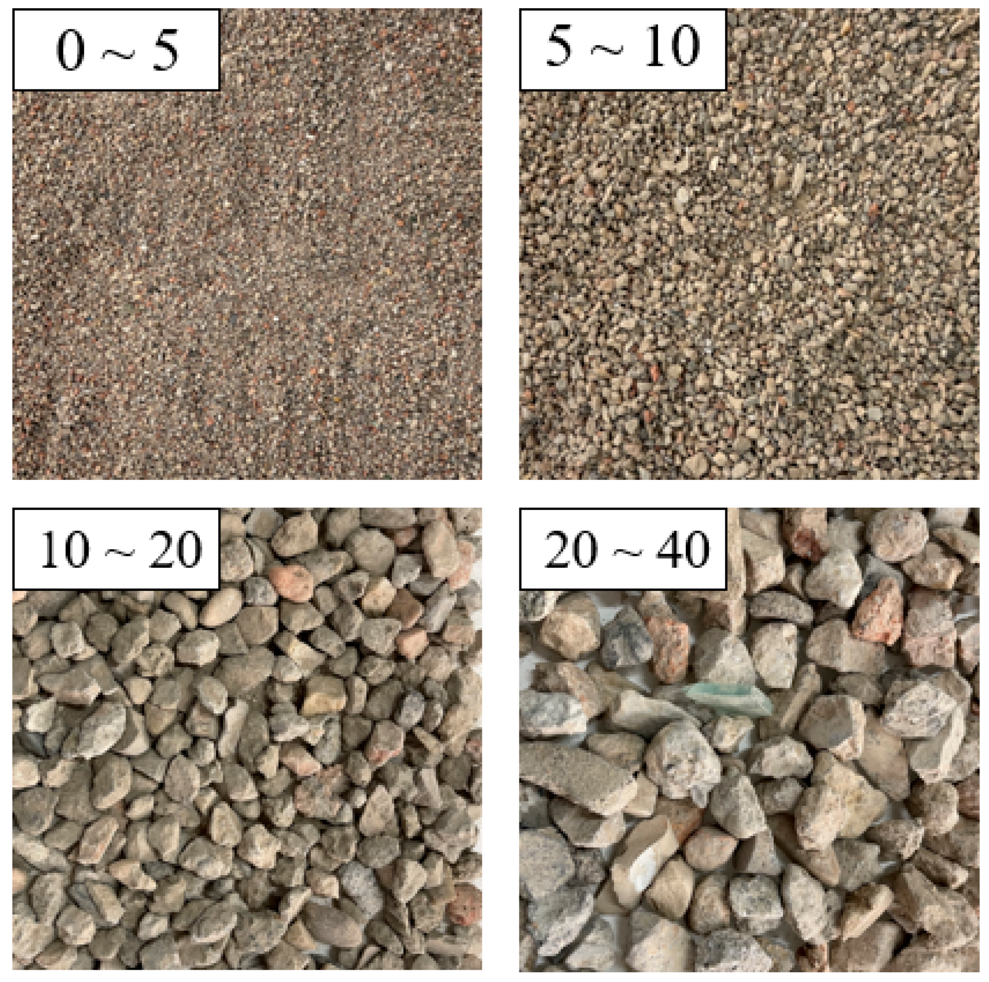
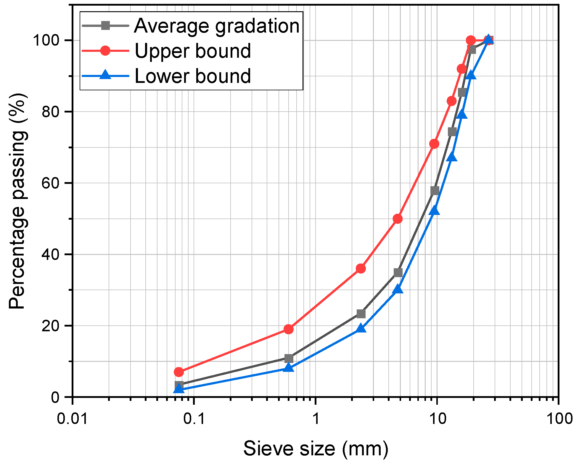
2.1. Tested Materials

The study employed two different aggregate materials, CDW and VA, in varying ratios. These materials were collected from the Yunzhong Company in Changsha, China, producing VA and recycled waste from building demolitions and other city infrastructure. The recycled materials from building demolition include used bricks, mortar, aggregates, and other elements such as wood, plastics, glass, paper, and others. For this study, these substances underwent crushing and screening to remove undesired elements, including wood, plastics, glass, paper, etc.; the main composition ratio of CDW used in this study are shown in

Table 1. Proportion by mass of the CDW.

Size	Gravel	Mortar	Brick	Others (Tiles, Wood, Nails, and Others)
5–10	65.78	24.65	8.34	1.23
10–20	69.58	17.80	7.93	4.69
20–40	68.93	23.72	5.21	2.14

. Then they were sorted into various sizes, as depicted in Figure 1. The blending proportions used in this study were as follows: 0% CDW and 100% VA, 65% CDW and 15% VA, 85% CDW and 35% VA, and 100% CDW and 0% VA. The grain size distribution was determined according to the JTG/T-F20-2015 standard [42], as illustrated in Figure 2.

Table 2. Basic index properties of the blended CDW.

Percentage of CDW (%)	Specific Gravity	Absorption (%)	Maximum Dry Density (g/cm3)	Optimum Moisture Content (%)	Apparent Cohesion c’ (kPa)	Internal Friction Angle (°)
0	2.697	0.302	2.238	5.5	87.4	51.7
65	2.406	3.715	2.040	7.0	59.1	52.1
85	2.402	3.763	2.063	6.0	59.5	54.8
100	2.370	3.945	1.958	6.4	41.2	52.4

summarizes the critical index characteristics of the blended CDW based on specific gravity, absorption, compaction, and undrained shear strength tests. The compaction characteristics of the four possible combinations were evaluated following Chinese standards (JTG 3430-2020) [43]. The compaction test parameters are listed in

Table 3. Laboratory compaction test parameters according to Chinese standard (JTG 3430-2020).

Test Method	Specimen Height (cm)	Specimen Volume (cm3)	Sub-Layers	Blows per Sub-Layer	Hammer Weight (kg)	Falling Height (mm)	Maximum Particle Size (mm)
Heavy II-2	12	2177	3	98	4.5	450	40

.

2.2. Repeated Load Triaxial Test

The mechanical performance of the blended CDW was evaluated using a series of repeated load triaxial tests. These tests were conducted using an MTS automated apparatus. The specimen was created in a split mold with 100 mm in diameter and 300 mm in height. The optimum moisture content and the maximum dry density obtained from the compaction test were utilized to prepare the samples. Four separate layers of the sample were placed into the split mold and compacted to a relative compaction of 95%. In order to prevent the sample from collapsing during the preparation and loading phases, a 0.5 mm-thick latex membrane was placed over the specimen.

The performance of a pavement depends on several factors: traffic volume, soil characteristics, depth of the subgrade, and varying amplitude and frequency of dynamic stresses. Therefore, this study used three levels of confining pressure: 50, 100, and 150 kPa. Given that the typical confining pressure experienced in unbound granular base materials ranges from 12.65 to 99.1 kPa, it is crucial to note that the high confining pressure used in this study aimed to replicate a base/subbase course that can handle severe traffic loading [44,45]. The concept of the shear stress ratio, proposed by Chow in 2014 [46], was utilized to calculate the deviator stress using four different SSR values: 0.3, 0.5, 0.7, and 0.9, corresponding to low, medium, high, and extreme stress levels. The Mohr–Coulomb criterion, depicted in Figure 3, defines the SSR as the ratio of shear stress to shear strength, as shown in Equations (1)–(4). The time-history curve of axial stress and the loading waveform of half-sine with a frequency of 5 Hz is depicted in Figure 4. The specimen was subjected to 50,000 load cycles to simulate long-term traffic loading. The testing matrix of physical and loading parameters of the CDW specimens under repeated load triaxial tests is shown in

Table 4. The testing matrix of physical and loading parameters adopted for repeated load triaxial tests.

Specimen Designation	Moisture Condition (%)	Confining Pressure σ3 (kPa)	Shear Stress Ratio (SSR)	Deviator Stress σd (kPa)	No. of Load Applications (N)
100% CDW	wopt	50	0.3/0.5/0.7/0.9	120.3/223.3/352.6/519.9	50,000
100% CDW	wopt	100	0.3/0.5/0.7/0.9	193.9/359.9/568.4/838.0.	50,000
100% CDW	wopt	150	0.3/0.5/0.7/0.9	267.5/496.5/784.1/1156.1	50,000
85% CDW + 15% VA	wopt	50	0.3/0.5/0.7/0.9	156.9/291.8/462.1/683.9	50,000
85% CDW + 15% VA	wopt	100	0.3/0.5/0.7/0.9	242.2/450.4/713.4/1055.7	50,000
85% CDW + 15% VA	wopt	150	0.3/0.5/0.7/0.9	327.4/609.0/964.6/1427	50,000
65% CDW + 35% VA	wopt	50	0.3/0.5/0.7/0.9	138.8/257.6/406.6/599.3	50,000
65% CDW + 35% VA	wopt	100	0.3/0.5/0.7/0.9	211.1/391.7/618.4/911.3	50,000
65% CDW + 35% VA	wopt	150	0.3/0.5/0.7/0.9	283.5/25.8/830.1/1223.4	50,000
0% CDW	wopt	50	0.3/0.5/0.7/0.9	168.1/311.7/491.8/724.4	50,000
0% CDW	wopt	100	0.3/0.5/0.7/0.9	238.7/442.6/698.4/1028.6	50,000
0% CDW	wopt	150	0.3/0.5/0.7/0.9	309.3/573.6/905.0/1332.9	50,000
85% CDW + 15% VA	wopt ± 1	50	0.3/0.5/0.7	156.9/291.8/462.1	50,000
85% CDW + 15% VA	wopt ± 1	100	0.3/0.5/0.7	242.2/450.4/713.4	50,000
85% CDW + 15% VA	wopt ± 1	150	0.3/0.5/0.7	327.4/609.0/964.6	50,000
65% CDW + 35% VA	wopt ± 1	50	0.3/0.5/0.7	138.8/257.6/406.6	50,000
65% CDW + 35% VA	wopt ± 1	100	0.3/0.5/0.7	211.1/391.7/618.4	50,000
65% CDW + 35% VA	wopt ± 1	150	0.3/0.5/0.7	283.5/25.8/830.1	50,000

.

$$SSR=\frac{{\tau }_f}{{\tau }_{\max }},$$

(1)

$${\tau }_f=\frac{{\sigma }_d\cos \phi }{2},$$

(2)

$${\tau }_{\max }={\sigma }_f\tan \phi +c,$$

(3)

$${\sigma }_f={\sigma }_3+\frac{{\sigma }_d(1-\sin \phi )}{2},$$

(4)

where τ_f is the shear stress (kPa) on the shear plane when the shear failure occurs; τ_max is the shear strength (kPa) of the sample under a specific stress state; σ_d is the amplitude of the deviator stress (kPa); σ_f is the normal stress (kPa) on the shear plane when the shear failure occurs; φ is the angle of internal friction (in °); c is cohesive of the soil (kPa); σ₃ is the confining pressure.

3. Laboratory Testing Results

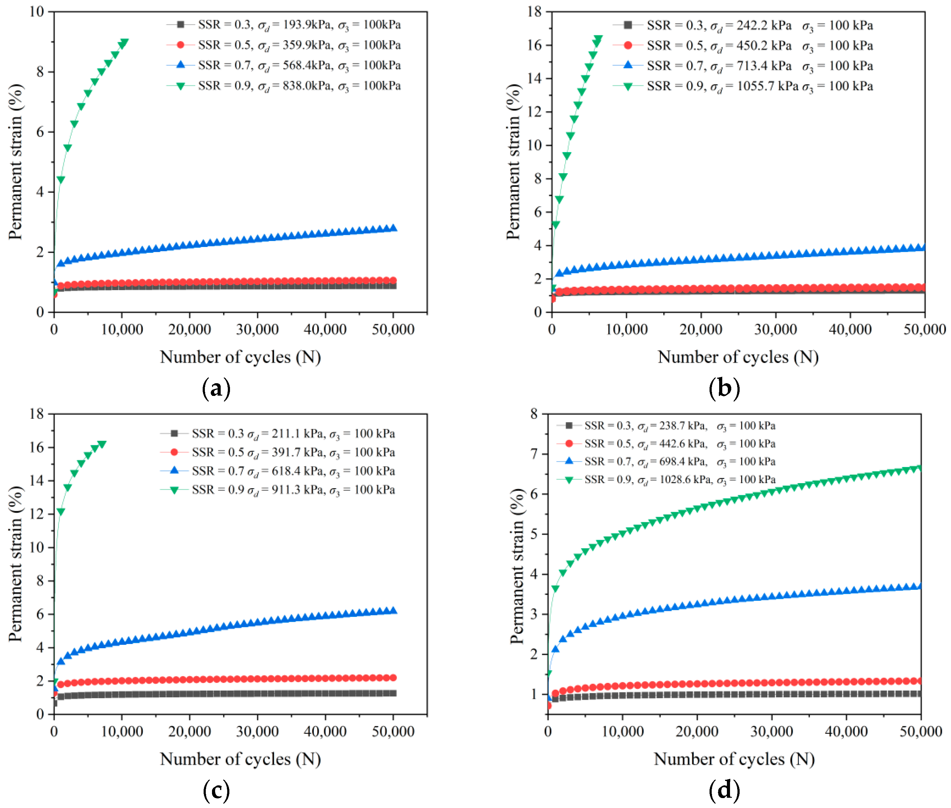
3.1. Effect of Shear Stress Ratio

The cumulative axial strain of the blended construction demolition and VA at a confining pressure of 100 kPa and various SSR levels is illustrated in Figure 5 as a function of the loading cycles. Figure 5a displays that as the SSR level rises, the permanent deformation of the materials increases. Applied stresses are far from the failure stage of the blends. At this stress level, the aggregates undergo rapid deformation at the initial loading cycles, which gradually cease to increase as the loading cycles progress, thereby becoming stable. This rapid deformation resulted from the compaction rearrangement and packing of the aggregate particles. The particles become entirely resilient as the number of loading cycles increases because they have reached a steady-state condition. The accumulation of plastic strain is rapid at the initial application of the stress, which continues to accumulate slowly until the end of the loading cycles. The specimen at this stage does not seem stable and can be classified as critical. Cumulative axial strain accelerated rapidly up to the failure stage, primarily at a few loading cycles. The blends failed at this SSR level because the stress level was beyond their bearing strength, and they could no longer resist the imposed stress.

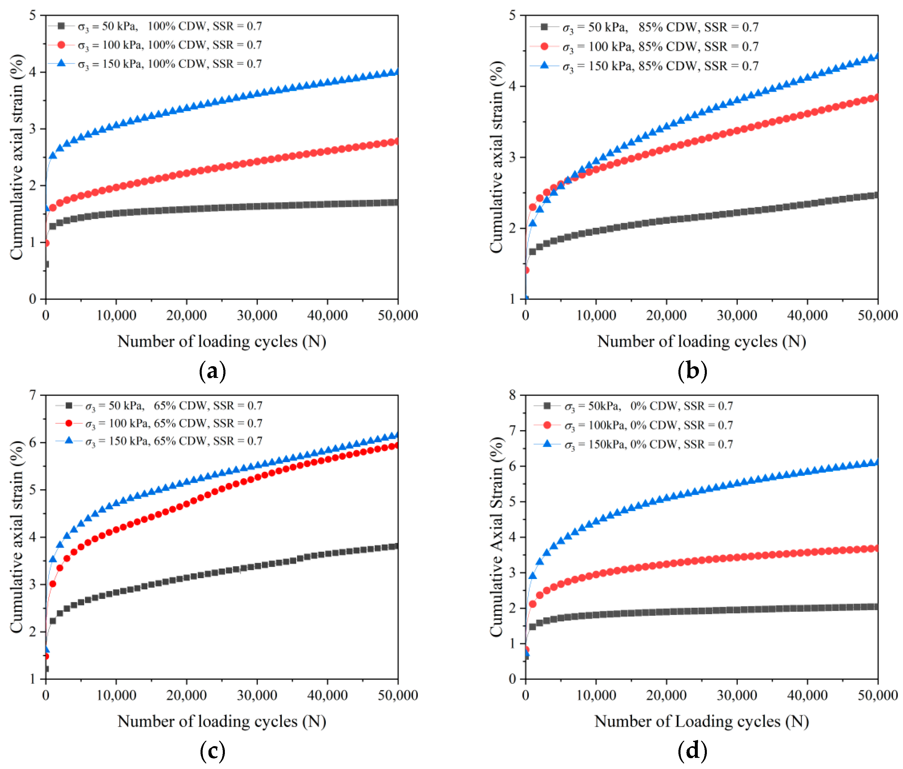
3.2. Effect of Confining Pressure

The development behaviors of the axial strain for the blended aggregates under different test conditions were similar. Therefore, only the curves of the blended aggregates at SSR (SSR = 0.7) are depicted. Figure 6 illustrates the relationship between the cumulative axial strain and the number of loading cycles, depicting the confining pressure effect on the accumulated axial strain. The axial strain grows as the confining pressure increases, as shown in Figure 6. This result contradicts existing ones where the confining pressure reduces the material’s tendency to undergo rapid deformation. This trend is observed in all the samples, in which as the confining pressure rises, the stress level also increases, increasing the accumulation of axial strain. This occurs because, based on the concept of SSR, as the confining pressure increases, the deviator stress also grows. A similar result was obtained by Ren et al. [44], which indicated that the ultimate axial strain develops as the confining pressure increases.

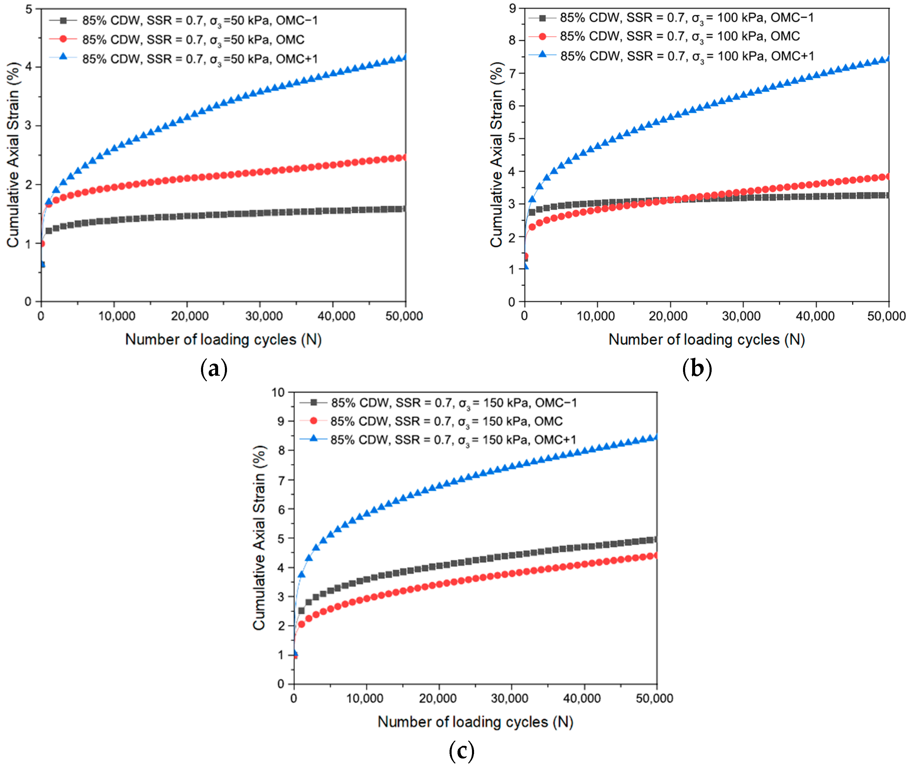
3.3. Effect of Moisture Content Variation

Figure 7 and Figure 8 display the relationship between the cumulative axial strain and the number of loadings, indicating the influence of moisture variation on the accumulated axial strain. The results reveal that moisture content significantly impacts the permanent deformation of the blended construction and demolition waste material when subjected to repeated cyclic loading. Specimens with moisture content below the optimum moisture content (OMC) exhibit good resistance to permanent deformation, whereas those above the OMC undergo substantial deformations. These outcomes can be attributed to aggregate inter-particle interactions under varying moisture conditions. As the moisture content rises, the inter-particle friction reduces, decreasing the shear strength and increasing the permanent deformation of the blended aggregates. The discrete nature of the components in the CDW should be noted, as it leads to significant fluctuations in the strain curves of certain test samples. For example, in Figure 6b, Figure 7b, and Figure 8b, the strain curve exhibits fluctuations. As shown in Figure 6b, the cumulative axial strain of the specimen during the pre-test period at σ₃ = 100 kPa is actually higher than that of the specimen tested at σ₃ = 150 kPa. This phenomenon can be attributed to the complex composition of the CDW, where the components have varying mechanical properties. The presence of impurities with poor mechanical properties in the specimen makes it more susceptible to deformation, thus reducing its overall resistance to deformation.

4. ANN Model Development

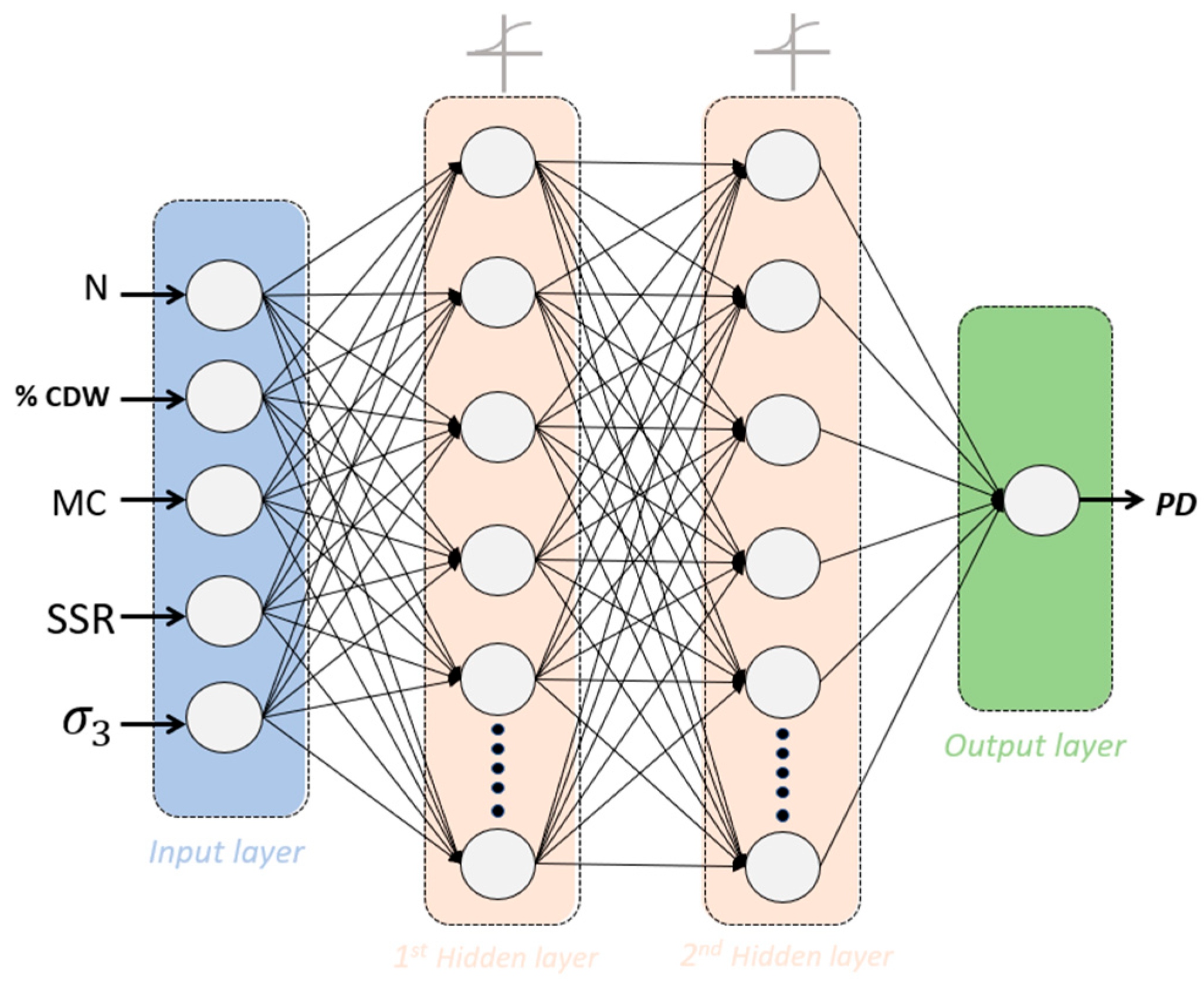
4.1. ANN Model Architecture

The ANN draws inspiration from the biological nervous system, i.e., the brain’s information processing mechanism. The ANN comprises numerous artificial neurons, referred to as processing elements. These elements are extensively interconnected, essential for producing an efficient output [47,48,49]. The neural network can learn from experience and information to enhance its performance. In multilayer perceptions, processing elements are organized in layers, including input, output, and one or more intermediate layers, known as hidden layers. These hidden layers contain neurons that determine patterns and the relationships between the output and the input [50], which can approximate any measurable function with a desired accuracy by employing a sufficient number of hidden neurons [51]. In each hidden layer, the input variables are multiplied by the weights and summed, and a bias value is added to the system [21], as shown in Equation (5).

$$O=f_o\left\{b_0+{\displaystyle \sum _{k=1}^q{w}_k^0{f}_h\left[b_k^{2h}+{\displaystyle \sum _{j=1}^n{w}_{jk}^{2h}{f}_h(b_j^{1h}+{\displaystyle \sum _{i=1}^m{w}_{ij}^{1h}{p}_i})}\right]}\right\},$$

(5)

where O is the output value; f_o is the transfer function for the output layer; b₀ is the bias factor for the output layer; $w_k^0$ is the weight factor for the output layer; f_h is the transfer function for the hidden layers; $b_k^{2h}$ is the bias factors for the second hidden layer; $w_{jk}^{2h}$ is the weight factor for the second hidden layer; $b_j^{1h}$ is the bias factor for the first hidden layer; $w_{ij}^{1h}$ is the weight factor for the first hidden layer; p_i is the input variables; k is the code for the second hidden layer; j is the code for the first hidden layer; i is the code for input layer; q is the number of neurons in the second hidden layer; n is the number of hidden neurons; m is the number of the input parameters.

The effectiveness of the ANN model depends on the number of hidden layers and neurons. A few neurons can decrease the model’s robustness if it hampers the model from correctly fitting the data. Conversely, excess hidden neurons can lead to overfitting and significant testing errors [29,41,52]. There is no standard method for determining the optimal ANN architecture that can accurately predict the outcome. Some researchers maintain that a three-layer network suffices for solving any complex nonlinear problem [52,53,54], while others argue that it depends on the nature of the dataset and the problem’s complexity [41].

Several scholars suggest that the trial-and-error method remains the most effective approach when determining the ideal number of hidden layers and neurons [55]. Despite the absence of a direct and precise method, some general guidelines exist to minimize computational time, ensure better generalization, and prevent overfitting. The optimal strategy is to begin with a few nodes and gradually increase the number until no significant improvement in model performance is observed. However, for networks with two hidden layers [56], the geometric pyramid rule, where the number of neurons in each layer follows the geometric progression of a pyramid, decreasing from the input layer toward the output layer, is the best approach. As shown in

Table 5. Comparison of different ANN model architecture.

Model	Hidden Layer 1		Hidden Layer 2		MSE	RMSE	R2 Value
	Transfer Function	Number of Neurons	Transfer Function	Number of Neurons
1	Tansig	22	-	-	0.005200	0.0724	0.9990
2	Logsig	24	-	-	0.005100	0.0711	0.9989
3	Tansig	16	Tansig	4	0.008600	0.0929	0.9981
4	Tansig	16	Tansig	8	0.039600	0.1990	0.9915
5	Tansig	20	Tansig	4	0.000850	0.9998	0.9998
6	Tansig	20	Tansig	8	0.000150	1.0000	0.9999
7	Tansig	20	Tansig	12	0.000069	0.0083	0.9999
8	Tansig	24	Tansig	4	0.000150	0.0122	0.9999
9	Tansig	24	Tansig	8	0.000360	0.0189	0.9999
10	Tansig	24	Tansig	12	0.000210	0.0143	1.0000
11	Logsig	20	Logsig	4	0.029900	0.1728	0.9936
12	Logsig	20	Logsig	8	0.000103	0.0102	0.9999
13	Logsig	20	Logsig	12	0.000056	0.0075	0.9999
14	Logsig	24	Logsig	4	0.000750	0.0273	0.9998
15	Logsig	24	Logsig	8	0.000076	0.0087	0.9999
16	Logsig	24	Logsig	12	0.000022	0.0047	0.9999

, ANN models with different architectures were developed in this study to investigate the effects of the activation function, the number of hidden layers, and the number of neurons in each hidden layer on the prediction accuracy.

4.2. Data Preprocessing

The dataset used for the ANN model development in this study includes 84 experimental repeated load triaxial tests. MATLAB software was employed to process the dataset. The dataset was normalized based on the log-sigmoid function utilized in the ANN architecture, where all values range from 0 to 1 for the neural network analysis. The dataset was divided into 80% for training and 20% for testing. Five parameters, namely, the number of loading cycles, the content of construction and demolition waste, moisture content, SSR, and confining pressure, were considered as the input for the input layer, while the cumulative axial strain was the only output of the ANN model. As described in the Section 3, the permanent deformation of the blended CDW was highly correlated with the loading history (i.e., the number of loading cycles). Stress conditions can significantly affect the deformation of the material and at least two parameters are required to characterize the stress level in triaxial compression tests, and, thus, SSR and confining pressure were also selected as inputs. As demonstrated in Section 3.3, the blended CDW was found to be moisture sensitive through repeated load triaxial tests. As the primary properties of the studied materials, the CDW content was taken as an input together with the moisture content, reflecting the influence of internal factors on the permanent deformation. As proposed by previous researchers, the minimum ratio of the dataset over the number of input parameters for model acceptability is three [57]. However, a ratio greater than five is recommended. This study’s ratio for training and validation surpasses the proposed criteria.

In addition to minimizing the complexity of the dataset (e.g., the redundant input variable σ_d was not included in the inputs), the size of the dataset was simplified from N = 1, 2, …, 50,000 to N = 10, 20, …, 50,000 in order to reduce the training time of the neural network. On the other hand, to predict the permanent deformation of the material as accurately as possible for a small number of loading cycles, it was decided to use the dataset of the above size. However, further research is still needed to balance the size of the dataset and the prediction accuracy of the neural network.

4.3. ANN Learning Algorithm

This study employed the multilayer feed-forward network with a backpropagation algorithm. Several training algorithms exist, such as Bayesian regularization, Conjugate gradient, Gradient descent, Levenberg–Marquardt, Quasi-Newton algorithms, and others. For multilayer perception networks with moderate-size weights and biases used for function approximation, the Levenberg–Marquardt algorithm is the fastest. It performs better on function fitting but requires high memory and more computation time for networks with high weights (in the thousands). The algorithm is assumed to converge when the sum of squares is reduced to a specific error. The Levenberg–Marquardt algorithm is deemed suitable for this study due to its speed and the size of the datasets.

4.4. Transfer Function

Different transfer functions are used for training multilayer perception networks. These functions add nonlinearity to the neural network, enhancing the network’s learning process. Log-sigmoid, tan-sigmoid, and purelin are three commonly applied transfer functions. Purelin is a linear activation function used for the output layer, whereas log-sigmoid and tan-sigmoid are nonlinear functions used between the input and hidden layers. The log-sigmoid transfer function, as described in Equations (6) and (7), is considered appropriate for this study.

Log-sigmoid:

$$f(x)=\frac{1}{1+e^{-x}},$$

(6)

Purelin:

$$f(x)=x,$$

(7)

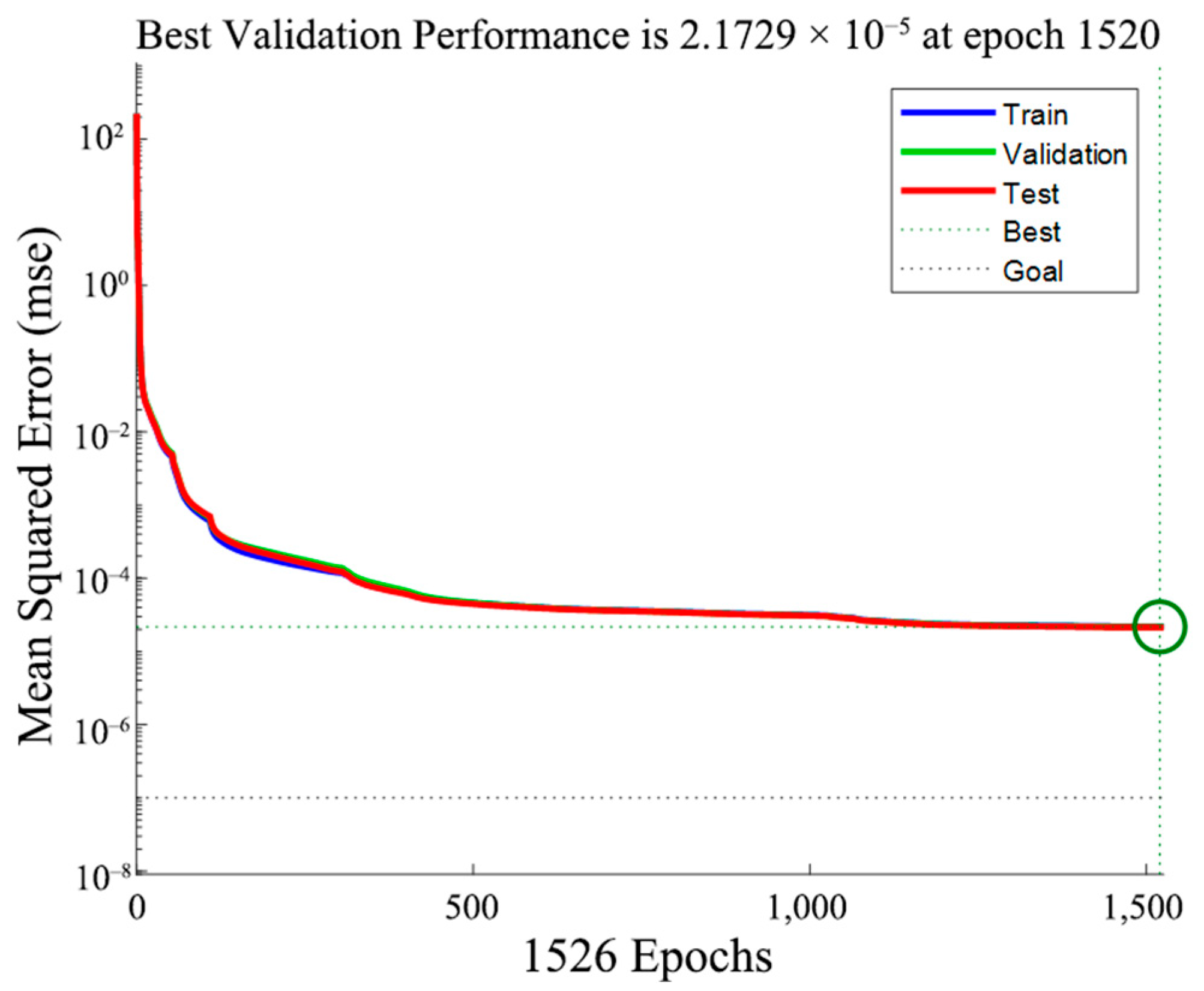
4.5. Stopping Criteria

The stopping criterion is a significant factor that profoundly influences the training process. Insufficient training often results in the network’s high tendency to produce inaccurate predictions [39]. In multilayer networks, the error is unlikely to reach zero, necessitating specific criteria to determine when to halt training. This study specified a fixed number of iterations and set a defined limit for the error, terminating the training upon reaching this limit.

4.6. ANN Model Performance Criteria

The ANN model strives to deliver the best fitness value for learning and validation datasets. The correlation coefficient does not accurately represent the predictive model [58,59]. Alongside the regression coefficient, the neural network’s stability is evaluated through error measurement. A minimal error indicates better stability, while a higher error reflects weaker or unstable stability [29]. The study assesses the performance of the proposed ANN model by utilizing statistical approaches such as the coefficient of determination (R²), mean square error (MSE), root-mean-square error (RMSE), and mean absolute error (MAE). These statistical indexes aid in determining the best model architecture. These parameters are defined below in Equations (8)–(11):

MSE:

$$MSE=\frac{1}{n}{{\displaystyle {\sum }_{i=1}^n\left(O_i-{\hat{\mathrm{O}}}_i\right)}}^2,$$

(8)

RMSE:

$$RMSE=\sqrt{\frac{1}{n}{{\displaystyle {\sum }_{i=1}^n\left(O_i-\widehat{O_i}\right)}}^2},$$

(9)

Coefficient of determination:

$$R^2=1-\frac{{{\displaystyle {\sum }_{i=1}^n\left(O_i-{\hat{O}}_i\right)}}^2}{{\displaystyle {\sum }_{i=1}^n{\left(O_i-{\hat{O}}_i\right)}^2}},$$

(10)

Mean absolute error:

$$MAE=\frac{1}{n}{\displaystyle \sum _{i=1}^n\left|O_i-{\hat{O}}_i\right|},$$

(11)

The process of training a neural network involves adjusting the weights and bias values of the network to optimize the network performance. In this paper, the Levenberg–Marquardt (LM) training algorithm and the mean square error (MSE) performance function were used. The MSE performance function is the mean squared error between the network output and the target outputs t, as defined in Equation (12). The LM algorithm updates the network weights and biases to approach second-order training speed without having to compute the Hessian matrix. The iteration of this algorithm can be written in the form shown in Equation (13).

$$F=mse=\frac{1}{N}{{\displaystyle \sum _{i=1}^N(e_i)}}^2=\frac{1}{N}{{\displaystyle \sum _{i=1}^N(t_i-a)}}^2,$$

(12)

$$x_k+1=x_k-{\left[{\mathrm{J}}^T\mathrm{J}+\mu \mathrm{I}\right]}^{-1}{\mathrm{J}}^{T}e,$$

(13)

where x_k is the current weights and biases, J is the Jacobian matrix that contains first derivatives of the network errors with respect to the weights and biases, e is the vector of current network errors, and μ is an adaptive value.

During training, Equation (12) will keep iterating while the performance value of the model will keep decreasing. As the training reaches a minimum of the performance, the gradient will become very small. If the magnitude of the gradient is less than the design value or the number of iterations is greater than the design value, the training will stop.

After training, test data are fed into the trained ANN to output the predicted values. Performance metrics such as R² are calculated based on the predicted and actual values. If the R² calculated on the test set is less than or equal to the value calculated on the training set, it means that the network can replicate the experimental results well and at the same time has a certain generalization ability (i.e., no overfitting occurs).

4.7. Optimum ANN Model Architecture

Table 5 demonstrates the impact of the number of hidden neurons and the transfer function within the hidden layers on the ANN models’ performance. MSE, RMSEs, and the R² were utilized to evaluate the models’ performance. As per Table 5, the model with a log-sigmoid transfer function and 24 and 12 neurons in the first and second layers, respectively, exhibits the most precise prediction and demonstrates satisfactory performance with the lowest values of MSE and RMSE and a high R2 value in comparison to the other models examined. The model’s optimal structure is displayed in Figure 9.

5. Result and Discussion

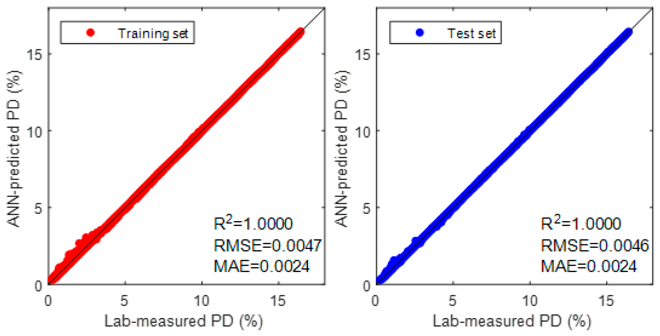
5.1. ANN Model Performance

Figure 10 presents the performance of the proposed ANN model, displaying three distinct curves representing training, validation, and test errors. The MSE at each epoch is computed, revealing that the MSE decreases with an increasing number of epochs until reaching a point where the validation error ceases to decrease. The model achieves the best validation error at epoch 1520, recorded as 2.1729 × 10⁻⁵. A detailed examination of the figure suggests that the error characteristics are similar, with no noticeable overfitting at epoch 1520, where the smallest MSE is observed.

Figure 11 illustrates the ANN model performance against the measured permanent deformation for the composite construction and demolition waste unbound granular aggregate. When the data align along the line of equity (line drawn at 45 degrees), the predicted values equal the actual values, suggesting perfect prediction. The goodness of fit between the predicted and the measured values is evaluated using R², which ranges between 0 and 1. When the R² is close to 1, perfect prediction is achieved. The figure above shows that the value of R² for both training and testing almost equals 1, indicating a perfect fit and an excellent performance of the ANN model with a strong correlation between the measured and predicted data. In addition, the MAE and the RMSE are within 0.0024 and 0.0047 for both training and testing datasets, indicating that the ANN model underpredicts the permanent deformations at an average of 0.0024 and the deviation between the experimental and predicted values is a significantly small 0.0047. A higher R² value and lower RMSE and MAE values denote better model performance. Therefore, the result indicates that the ANN model can replicate the laboratory-measured permanent deformation with high accuracy and precision.

Although the ANN model demonstrates robust and excellent predictive capabilities based on the performance criteria, it remains uncertain whether the model will maintain this excellent fitting when introducing an entirely new dataset. Therefore, external validation is required to ensure the model’s reliability [21]. The criteria proposed by [60,61] were utilized to assess and verify the developed model’s external validation. Four sets of criteria are employed to determine the model’s capability to perform well when external datasets are introduced. These criteria and their limits are defined in

Table 6. Statistical criteria for external validation of the ANN model.

Criterion	Limit	Result Obtained
$R_o^2=1-\frac{{\displaystyle {\sum }_{i=1}^n{\left(\hat{O}-O_i^o\right)}^2}}{{\displaystyle {\sum }_{i=1}^n{\left(\hat{O}-\stackrel{\stackrel{\_}{^}}{O}\right)}^2}}$	It should be close to R2	1.000
$R_o^{\prime 2}=1-\frac{{\displaystyle {\sum }_{i=1}^n{\left(\hat{O}-{\hat{O}}_i^o\right)}^2}}{{\displaystyle {\sum }_{i=1}^n{\left(\hat{O}-\stackrel{\stackrel{\_}{^}}{O}\right)}^2}}$	It should be close to R2	1.000
$m=\frac{R^2-R_o^2}{R^2}$	$\left|m\right|<0.1$	−8.0614 × 10−6
$n=\frac{R^2-R_o^{\prime 2}}{R^2}$	$\left|n\right|<0.1$	−8.0614 × 10−6
$R_m^2=R^2\left(1-\sqrt{\left|R^2-R_o^2\right|}\right)$	$0.5<R_m$	0.997
$k=\frac{{\displaystyle {\sum }_{i=1}^n{\left(O_i.{\hat{O}}_i\right)}^2}}{{\displaystyle {\sum }_{i=1}^n\left({\hat{O}}_i^2\right)}}$	$0.85\le k\le 1.15$	1.000
$k^{\prime }=\frac{{\displaystyle {\sum }_{i=1}^n{\left(O_i.{\hat{O}}_i\right)}^{}}}{{\displaystyle {\sum }_{i=1}^n\left(O_i^2\right)}}$	$0.85\le k\prime \le 1.15$	1.000

where $R_o^2$ and $R_o^{\prime 2}$ are the correlation coefficients of the lines through the origin; $R_m$ is the modified R²; $O_i^o$ and ${\hat{O}}_i^o$ are the regressions line through the origin, in which $O_i^o$ = k × ${\hat{O}}_{\mathrm{i}}$ and ${\hat{O}}_i^o$ = k × O_i, given k and k′ are the slope of the line through the origin.

. From the results, values of 1.0 are comparable to those of similar testing conditions, satisfying the requirements. Thus, the proposed model meets the criteria, proving that the model is capable of predicting an external dataset with similar testing conditions.

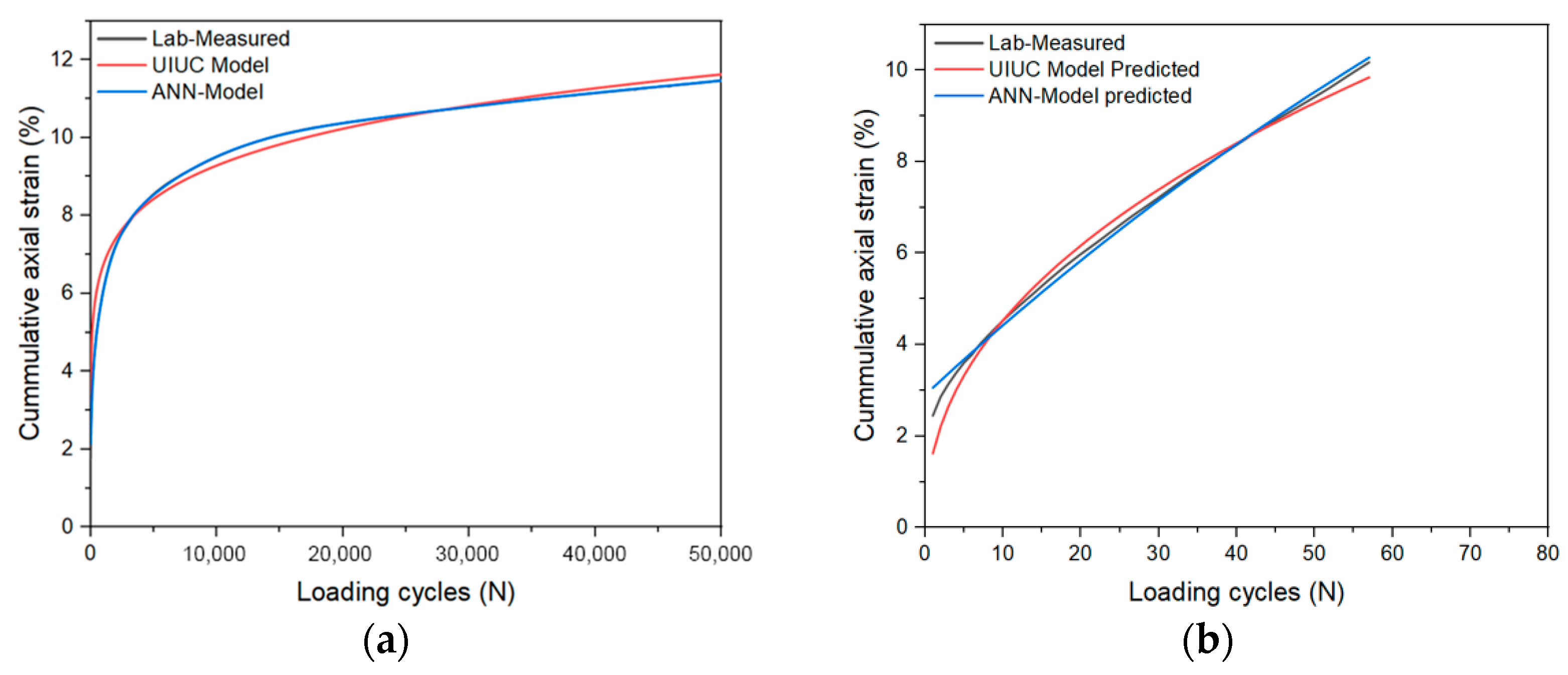
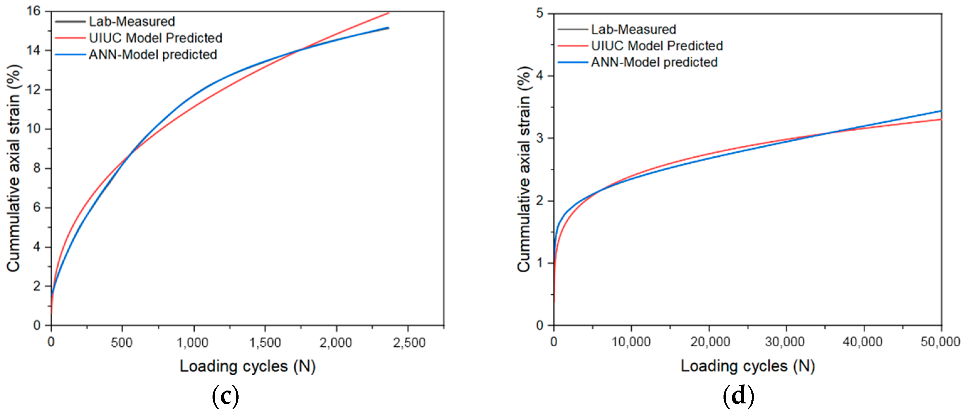
5.2. Comparison between the ANN Model and a Multiple Regression Model

Figure 12 exhibits the experimental results, the UIUC model’s predicted values, and the ANN model’s predicted values of the blended CDW aggregate materials. The robustness of the ANN model and the accuracy of the UIUC regression-based model proposed by Chow [46] are compared. Figure 11 compares the experimental and predicted values obtained from the ANN and UIUC models. It demonstrates that the ANN-predicted values are closer to the experimental values, indicating that the developed model successfully predicted the permanent strain of the blends considering different influencing factors. The result shows that the ANN model outperforms the regression-based model, demonstrating that the ANN model can describe the complex relationship between the input and output variables using neurons in the hidden layers.

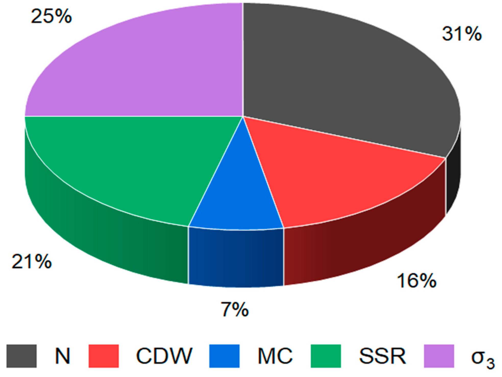
6. Sensitivity Analysis

Garson Algorithm

The sensitivity analysis method was applied to determine each input parameter’s contribution to the model. An increase in the quantity and complexity of input parameters enhances prediction accuracy [36,62]. However, the performance of prediction can be affected by irrelevant input values. As a result, sensitivity analysis was suggested for selecting appropriate input parameters based on relevance. The weights technique, developed by Garson (1991), is frequently employed to assess the relative significance of input parameters. This method partitions the hidden-output connection weights of each hidden neuron into components related to each input neuron. Garson’s algorithm uses the absolute values of the connection weights to compute the input contribution. Nevertheless, the structure of the ANN model influences this technique. For networks with multiple hidden layers, the contribution value of neurons in previous layers is impacted. Changes in the number of weights in each hidden layer will modify each neuron’s contribution. This study applied the extended version of Garson’s technique for multiple hidden layers, which computes and stores each hidden layer’s contribution values in a matrix after normalizing them all. The steps are summarized in Equations (14)–(17) below.

Normalization of the collected weight from successive layers:

$$\mathrm{w}=\left[\begin{array}{ccc}\frac{\left|w_{11}\right|}{{\displaystyle {\sum }_{i=1}^n\left|w_{i1}\right|}}& \cdots & \frac{\left|w_{1m}\right|}{{\displaystyle {\sum }_{i=1}^n\left|w_{im}\right|}}\\ ⋮& \ddots & ⋮\\ \frac{\left|w_{n1}\right|}{{\displaystyle {\sum }_{i=1}^n\left|w_{i1}\right|}}& \cdots & \frac{\left|w_{nm}\right|}{{\displaystyle {\sum }_{i=1}^n\left|w_{im}\right|}}\end{array}\right],$$

(14)

Multiplication of the normalized weight matrixes:

$$CW=w^1.w^2.w^3\dots w^L,$$

(15)

where w¹ represents the normalized weight matrix between the input layer and the output layer.

The multiplication is carried out till the final.

$$rc=\left[\begin{array}{c}{\displaystyle \sum _{j=1}^{n}C{W}_{1j}}\\ {\displaystyle \sum _{j=1}^{n}C{W}_{2j}}\\ ⋮\\ {\displaystyle \sum _{j=1}^{n}C{W}_{nj}}\end{array}\right],$$

(16)

The relative importance percentage can be obtained from the equation below.

$$rc=100\%\times \left[\begin{array}{c}\frac{r{c}_{11}}{{\displaystyle {\sum }_{i=1}^{n}r{c}_{i1}}}\\ \frac{r{c}_{21}}{{\displaystyle {\sum }_{i=1}^{n}r{c}_{i1}}}\\ ⋮\\ \frac{r{c}_{n1}}{{\displaystyle {\sum }_{i=1}^{n}r{c}_{i1}}}\end{array}\right],$$

(17)

It is generally believed that the weight value represents the degree of one neuron’s influence on another. The weight and bias values between the neurons in various layers of the optimal ANN model are shown in

Table 7. Weight and bias values in the first hidden layer of the ANN model.

No. of Neurons	${\mathit{w}}_{1\mathit{j}}^{1\mathit{h}}$	${\mathit{w}}_{2\mathit{j}}^{1\mathit{h}}$	${\mathit{w}}_{3\mathit{j}}^{1\mathit{h}}$	${\mathit{w}}_{4\mathit{j}}^{1\mathit{h}}$	${\mathit{w}}_{5\mathit{j}}^{1\mathit{h}}$	Bias
1	−0.1094	5.6973	−2.6239	−4.1142	−2.2875	−5.8412
2	−2.6531	−1.9948	−2.8745	−9.1333	−3.1458	7.2169
3	−0.6294	−1.6299	2.0106	3.6315	6.4585	2.3361
4	0.1171	0.5023	−0.0272	−2.4416	4.2335	−0.4899
5	0.3365	2.2900	4.2364	−5.0357	−3.2842	−5.2766
6	0.0737	1.0322	0.1258	0.0464	9.2983	9.7301
7	−0.3636	9.7478	−2.4388	14.0586	9.6219	3.9302
8	0.8907	2.1307	1.3836	7.1531	0.5404	−2.2487
9	0.4206	−8.8326	0.7155	−9.0036	−16.4121	12.2490
10	0.1758	−21.1393	−0.4254	0.5450	−1.1629	5.7882
11	0.5968	2.6394	0.1605	−1.1610	−2.2575	0.6746
12	0.2026	2.4468	3.5302	−8.1728	−4.4705	−1.2732
13	−0.1958	−12.5005	−8.0251	3.4476	−2.0155	0.9297
14	−0.2200	12.5328	−27.6076	−2.1199	−9.5615	−5.8104
15	0.1520	2.9182	−3.3135	−9.2082	0.7358	−5.6332
16	−0.6329	0.7560	−0.1534	−5.0035	0.9725	1.6679
17	4.2473	−0.0495	0.2003	−1.0546	−1.1639	6.2983
18	0.0824	−5.6410	−0.7707	−11.1252	13.6619	3.9059
19	−5.0133	3.6679	−0.6048	9.6750	1.8379	−12.1019
20	−0.0327	11.2124	−5.7675	−1.7260	10.8888	−7.9320
21	0.3489	−6.3274	1.1552	−5.0078	−19.4570	18.2258
22	27.8994	−1.3200	−0.7075	−3.6271	0.7454	30.8751
23	−17.6869	0.3266	0.8284	4.1171	0.2390	−22.2180
24	−73.0825	−0.1119	0.5436	0.9321	1.0957	−76.1978

,

Table 8. Weight and bias of the second hidden layer of the ANN model.

Number of Neurons	${\mathit{w}}_{1\mathit{k}}^{2\mathit{h}}$	${\mathit{w}}_{2\mathit{k}}^{2\mathit{h}}$	${\mathit{w}}_{3\mathit{k}}^{2\mathit{h}}$	${\mathit{w}}_{4\mathit{k}}^{2\mathit{h}}$	${\mathit{w}}_{5\mathit{k}}^{2\mathit{h}}$	${\mathit{w}}_{6\mathit{k}}^{2\mathit{h}}$	${\mathit{w}}_{7\mathit{k}}^{2\mathit{h}}$	${\mathit{w}}_{8\mathit{k}}^{2\mathit{h}}$	${\mathit{w}}_{9\mathit{k}}^{2\mathit{h}}$	${\mathit{w}}_{10\mathit{k}}^{2\mathit{h}}$	${\mathit{w}}_{11\mathit{k}}^{2\mathit{h}}$	${\mathit{w}}_{12\mathit{k}}^{2\mathit{h}}$	${\mathit{w}}_{13\mathit{k}}^{2\mathit{h}}$	${\mathit{w}}_{14\mathit{k}}^{2\mathit{h}}$	${\mathit{w}}_{15\mathit{k}}^{2\mathit{h}}$
1.	0.7146	−0.3988	2.4250	6.6116	0.6890	−6.9594	1.7063	−1.2343	−5.2970	−0.6711	3.0982	0.0161	4.2159	−1.1533	−0.5488
2.	−16.4659	2.2190	0.7273	6.7797	4.0228	−7.5493	0.9441	−15.6412	3.8110	−14.0547	−5.8514	−5.2285	−9.8674	1.9195	11.1362
3.	1.8968	−1.5852	1.8603	1.9031	2.4132	13.2439	2.0927	3.3924	−4.3266	−4.1764	0.4465	1.1636	−1.2214	−2.1732	−0.1646
4.	−2.7318	−0.2603	−1.1354	−0.2528	0.0820	−7.5951	1.4863	−0.2839	−3.3794	0.2096	−0.6990	−1.2705	0.1842	−1.1036	1.5444
5.	−0.5293	−3.8654	2.2891	10.5591	−9.9651	18.1215	−12.1999	1.7446	−1.7580	−2.7056	2.5688	−1.0575	−5.9527	6.1044	−5.4290
6.	2.6677	−3.0737	2.0298	6.9112	3.4642	−11.3896	3.7019	−6.1639	14.5756	2.4095	1.7059	1.0439	−4.5989	2.8452	0.1966
7.	0.5566	−5.5456	−2.8597	11.5208	2.0721	2.8176	1.2168	8.0306	−2.9587	−3.7244	2.1402	2.8904	−1.3286	1.0611	−5.0067
8.	−3.2716	1.5978	−1.6496	0.8116	−5.7029	−0.4009	−0.8204	−0.5505	4.5118	−1.3713	−3.8134	3.9949	−4.9466	1.7123	0.9079
9.	−4.7425	−3.0986	−7.1215	−12.1448	−0.3192	−14.2148	1.4936	2.0335	7.2961	2.3999	−2.0665	−1.4892	0.0024	4.1281	2.5828
10.	−1.6457	0.8667	−0.9029	−7.0424	−2.0925	1.0502	−2.9149	0.8246	3.7235	−3.6903	1.8387	1.0353	10.1864	−0.3438	−0.4639
11.	−4.0954	−0.6293	11.3081	−3.0892	2.3912	−10.0275	−7.3025	7.9210	2.4526	−8.9789	−1.8385	4.7274	12.4830	−2.8821	0.2723
12.	3.3456	−0.1275	0.6344	4.2034	4.5033	−4.8560	3.1607	−1.7153	2.0473	8.8093	6.8159	−5.3400	−5.6144	2.4990	−34.1919

and

Table 9. Weight and bias values in the second hidden layer of the ANN Model (continued).

Number of Neurons	${\mathit{w}}_{16\mathit{k}}^{2\mathit{h}}$	${\mathit{w}}_{17\mathit{k}}^{2\mathit{h}}$	${\mathit{w}}_{18\mathit{k}}^{2\mathit{h}}$	${\mathit{w}}_{19\mathit{k}}^{2\mathit{h}}$	${\mathit{w}}_{20\mathit{k}}^{2\mathit{h}}$	${\mathit{w}}_{21\mathit{k}}^{2\mathit{h}}$	${\mathit{w}}_{22\mathit{k}}^{2\mathit{h}}$	${\mathit{w}}_{23\mathit{k}}^{2\mathit{h}}$	${\mathit{w}}_{24\mathit{k}}^{2\mathit{h}}$	${\mathit{w}}_{25\mathit{k}}^{2\mathit{h}}$
1.	−0.6536	−0.4666	−1.6391	0.8160	−1.7547	5.8938	−0.8661	−7.3072	2.1186	6.8634
2.	−7.1168	4.2295	−6.3028	−4.7430	−4.0240	−5.8181	2.9287	−4.2561	−2.9766	24.5150
3.	6.0359	0.3560	−2.1268	2.4940	−3.2969	3.4366	−2.0608	−12.7921	−1.5496	−15.0832
4.	−1.8965	0.1715	−1.2868	−0.6701	0.4239	3.2045	0.0236	−2.8066	−0.1310	11.0606
5.	8.4488	3.2800	−7.7378	−6.8762	9.1786	2.8125	1.4265	−5.9075	−11.6221	−19.0318
6.	−5.4748	−0.8150	−0.4198	2.0685	−1.8596	−15.2934	0.0932	−7.4596	2.5995	6.5697
7.	−8.1357	12.6468	3.6756	−4.3331	−0.9245	6.7587	26.3563	26.0665	−60.2009	−24.0241
8.	3.3867	−2.0912	0.9286	−1.8435	−0.5058	−2.0781	−0.7201	−2.3558	2.4062	3.5620
9.	5.5772	−2.9913	6.6608	−2.5804	4.0340	−4.3462	0.2886	19.7329	7.1202	6.1357
10.	3.2732	0.7859	7.6699	−1.0107	−0.3832	−4.0689	−0.2181	−2.7736	−2.3277	−4.8548
11.	−0.1646	7.6401	−10.1064	3.2279	1.0123	−12.8508	1.2497	3.9537	−4.1822	−0.8310
12.	−2.8282	1.8739	−0.4615	3.6850	−2.3380	−5.9040	−0.1491	−3.9433	0.0691	−2.2141

, which can be accessed by readers to use and further improve the developed ANN. The relative significance of the input variables to the predicted permanent deformation can be deduced from these values using Equations (14)–(17). Figure 13 displays the influence of input parameters on the model for permanent deformation prediction. The results indicate that all the input parameters are crucial for predicting permanent deformation. The number of loading cycles with a 31% influence strongly impacts the output variable, followed by confining pressure and the SSR with 25% and 21% influence, respectively. The impact of the construction and demolition waste content was more substantial than the moisture content. The findings indicate that testing conditions and materials play a significant role in deformation, guiding policymakers and practitioners in regulating the use of these materials and ensuring proper pavement maintenance.

7. Conclusions

This study focuses on developing an ANN-based model to predict the permanent deformation behavior of blended CDW. Experimental data from laboratory repeated load triaxial tests are employed to train further and validate the ANN model. The conclusions drawn from the obtained results can be summarized as follows:

• The repeated load triaxial tests indicated that the newly developed matrix of blended aggregates could serve adequately as base or subbase materials under traffic loading. The SSR and deviator stress significantly influence the deformation behavior of the CDW materials. The effects of deviator stress, confining pressure, and moisture content are more noticeable at a high SSR (e.g., SSR = 0.7) compared to a lower SSR (e.g., SSR = 0.5). The blended materials showed sensitivity to moisture variation, with moisture content above the optimum producing considerable permanent strain.
• The ANN model was proposed to predict the permanent deformation of blended CDW and VA. Due to the material’s complexity and the dataset’s enormous size, the optimum neural network determined in this study was a four-layered network with two hidden layers. The complexity associated with the CDW was fully incorporated into the model. The ANN model demonstrated a high degree of accuracy, with an average coefficient of determination of 0.99.
• The performance criteria of the developed ANN model indicate its capability to predict the permanent deformation of the blended proportions with high precision and accuracy. Additional performance criteria were utilized to determine the model’s applicability to predict its performance when applied to an external dataset. The results confirmed the model’s adequacy in predicting the permanent deformation of external data.
• The comparison between the ANN-based and regression-based models revealed that the ANN model outperforms conventional regression-based models. The ANN model, accommodating various combinations of input parameters at any given loading application, can predict the accumulative permanent strain more efficiently than the regression model, with improved computation time. Most regression-based models rely on specified equations that involve tedious linear and nonlinear calculations.
• The ANN model surpasses the regression-based model by determining each input parameter’s contribution through network weights via sensitivity analysis. The result indicated that all the selected input parameters influence the accuracy of the permanent deformation model.
• Sensitivity analysis revealed that all input parameters are essential for predicting permanent deformation. Testing parameters such as the number of loading cycles, confining pressure, and SSR significantly control the permanent deformation behavior of the materials. With a total sensitivity coefficient close to 80%, the loading condition greatly affects the permanent deformation behavior of the blended CDW. The content of construction and demolition waste and moisture content also play roles in determining the material’s response.

References

1. Li, X.P. Recycling and reuse of waste concrete in China Part I. Material behaviour of recycled aggregate concrete. Resour. Conserv. Recycl. 2008, 53, 36–44. [Google Scholar] [CrossRef]
2. Zheng, L.N.; Wu, H.Y.; Zhang, H.; Duan, H.; Wang, J.; Jiang, W.; Dong, B.; Liu, G.; Zuo, J.; Song, Q. Characterizing the generation and flows of construction and demolition waste in China. Constr. Build. Mater. 2017, 136, 405–413. [Google Scholar] [CrossRef]
3. Lee, J.C.; Edil, T.B.; Tinjum, J.M.; Benson, C.H. Quantitative assessment of environmental and economic benefits of recycled materials in highway construction. Transp. Res. Rec. 2010, 2158, 138–142. [Google Scholar] [CrossRef]
4. Mills-Beale, J.; You, Z.P. The mechanical properties of asphalt mixtures with Recycled Concrete Aggregates. Constr. Build. Mater. 2010, 24, 230–235. [Google Scholar] [CrossRef]
5. Arulrajah, A.; Ali, M.M.Y.; Piratheepan, J.; Bo, M.W. Geotechnical Properties of Waste Excavation Rock in Pavement Subbase Applications. J. Mater. Civ. Eng. 2012, 24, 924–932. [Google Scholar] [CrossRef]
6. Arulrajah, A.; Piratheepan, J.; Disfani, M.M. Reclaimed asphalt pavement and recycled concrete aggregate blends in pavement subbases: Laboratory and field evaluation. J. Mater. Civ. Eng. 2014, 26, 349–357. [Google Scholar] [CrossRef]
7. Cardoso, R.; Silva, R.V.; de Brito, J.; Dhir, R. Use of recycled aggregates from construction and demolition waste in geotechnical applications: A literature review. Waste Manag. 2016, 49, 131–145. [Google Scholar] [CrossRef]
8. Behiry, A.E.A.E.-M. Utilization of cement treated recycled concrete aggregates as base or subbase layer in Egypt. Ain Shams Eng. J. 2013, 4, 661–673. [Google Scholar] [CrossRef]
9. Gabr, A.R.; Cameron, D.A. Permanent Strain Modeling of Recycled Concrete Aggregate for Unbound Pavement Construction. J. Mater. Civ. Eng. 2013, 25, 1394–1402. [Google Scholar] [CrossRef]
10. Jiménez, J.R.; Ayuso, J.; Agrela, F.; López, M.; Galvín, A.P. Utilisation of unbound recycled aggregates from selected CDW in unpaved rural roads. Resour. Conserv. Recycl. 2012, 58, 88–97. [Google Scholar] [CrossRef]
11. Lim, S.; Zollinger, D.G. Estimation of the Compressive Strength and Modulus of Elasticity of Cement-Treated Aggregate Base Materials. In Proceedings of the 82nd Annual Meeting of the Transportation-Research-Board, Washington, DC, USA, 12–16 January 2003. [Google Scholar] [CrossRef]
12. Melbouci, B. Compaction and shearing behaviour study of recycled aggregates. Constr. Build. Mater. 2009, 23, 2723–2730. [Google Scholar] [CrossRef]
13. Vegas, I.; Ibañez, J.A.; Lisbona, A.; De Cortazar, A.S.; Frías, M. Pre-normative research on the use of mixed recycled aggregates in unbound road sections. Constr. Build. Mater. 2011, 25, 2674–2682. [Google Scholar] [CrossRef]
14. Arulrajah, A.; Piratheepan, J.; Disfani, M.M.; Bo, M.W. Geotechnical and Geoenvironmental Properties of Recycled Construction and Demolition Materials in Pavement Subbase Applications. J. Mater. Civ. Eng. 2013, 25, 1077–1088. [Google Scholar] [CrossRef]
15. Azam, A.M.; Cameron, D.A. Geotechnical Properties of Blends of Recycled Clay Masonry and Recycled Concrete Aggregates in Unbound Pavement Construction. J. Mater. Civ. Eng. 2013, 25, 788–798. [Google Scholar] [CrossRef]
16. Jayakody, S.; Gallage, C.; Ramanujam, J. Effects of reclaimed asphalt materials on geotechnical characteristics of recycled concrete aggregates as a pavement material. Road Mater. Pavement Des. 2019, 20, 754–772. [Google Scholar] [CrossRef]
17. Li, X.P. Recycling and reuse of waste concrete in China. Resour. Conserv. Recycl. 2009, 53, 107–112. [Google Scholar] [CrossRef]
18. Silva, R.V.; Brito, J.; Dhir, R.K. Properties and composition of recycled aggregates from construction and demolition waste suitable for concrete production. Constr. Build. Mater. 2014, 65, 201–217. [Google Scholar] [CrossRef]
19. Gomez-Meijide, B.; Pérez, I. Nonlinear elastic behavior of bitumen emulsion-stabilized materials with C&D waste aggregates. Constr. Build. Mater. 2015, 98, 853–863. [Google Scholar] [CrossRef]
20. Cerni, G.; Cardone, F.; Virgili, A.; Camilli, S. Characterisation of permanent deformation behaviour of unbound granular materials under repeated triaxial loading. Constr. Build. Mater. 2012, 8, 79–87. [Google Scholar] [CrossRef]
21. Ghorbani, B.; Arulrajah, A.; Narsilio, G.; Horpibulsuk, S.; Bo, M.W. Dynamic characterization of recycled glass-recycled concrete blends using experimental analysis and artificial neural network modeling. Soil Dyn. Earthq. Eng. 2021, 142, 106544. [Google Scholar] [CrossRef]
22. Li, Y.; Nie, R.; Yue, Z.; Leng, W.; Guo, Y. Dynamic behaviors of fine-grained subgrade soil under single-stage and multi-stage intermittent cyclic loading: Permanent deformation and its prediction model. Soil Dyn. Earthq. Eng. 2021, 142, 106548. [Google Scholar] [CrossRef]
23. Nie, R.; Mei, H.; Leng, W.; Ruan, B.; Li, Y.; Chen, X. Characterization of permanent deformation of fine-grained subgrade soil under intermittent loading. Soil Dynam. Earthq. Eng. 2020, 139, 106395. [Google Scholar] [CrossRef]
24. Orosa, P.; Medina, L.; Fernández-Ruiz, J.; Pérez, I.; Pasandín, A.R. Numerical simulation of the stiffness evolution with curing of pavement sections rehabilitated using cold in-place recycling technology. Constr. Build. Mater. 2022, 335, 127487. [Google Scholar] [CrossRef]
25. Sakhare, A.; Farooq, H.; Nimbalkar, S.; Dodagoudar, G.R. Dynamic Behavior of the Transition Zone of an Integral Abutment Bridge. Sustainability 2022, 14, 4118. [Google Scholar] [CrossRef]
26. Beale, M.H.; Hagan, M.T.; Demuth, H.B. Neural Network ToolboxTM User’s Guide; The MathWorks, Inc.: Natick, MA, USA, 2017. [Google Scholar]
27. Pazuki, G.R.; Nikookar, M.; Dehnavi, M.; Al-Anazi, B. The Prediction of Permeability Using an Artificial Neural Network System. Pet. Sci. Technol. 2012, 30, 2108–2113. [Google Scholar] [CrossRef]
28. Williams, C.G.; Ojuri, O.O. Predictive modelling of soils’ hydraulic conductivity using artificial neural network and multiple linear regression. SN Appl. Sci. 2021, 3, 152. [Google Scholar] [CrossRef]
29. Taha, O.M.E.; Majeed, Z.H.; Ahmed, S.M. Artificial Neural Network Prediction Models for Maximum Dry Density and Optimum Moisture Content of Stabilized Soils. Transp. Infrastruct. Geotechnol. 2018, 5, 146–168. [Google Scholar] [CrossRef]
30. Bahmed, I.T.; Harichane, K.; Ghrici, M.; Boukhatem, B.; Rebouh, R.; Gadouri, H. Prediction of geotechnical properties of clayey soils stabilized with lime using artificial neural networks (ANNs). Int. J. Geotech. Eng. 2019, 13, 191–203. [Google Scholar] [CrossRef]
31. Sinha, S.K.; Wang, M.C. Artificial Neural Network Prediction Models for Soil Compaction and Permeability. Geotech. Geol. Eng. 2008, 26, 47–64. [Google Scholar] [CrossRef]
32. Sivrikaya, O. Comparison of Artificial Neural Networks models with correlative works on undrained shear strength. Eurasian Soil Sci. 2009, 42, 1487–1496. [Google Scholar] [CrossRef]
33. Mollahasani, A.; Alavi, A.H.; Gandomi, A.H.; Rashed, A. Nonlinear neural-based modeling of soil cohesion intercept. KSCE J. Civ. Eng. 2011, 15, 831–840. [Google Scholar] [CrossRef]
34. Kim, S.-H.; Yang, J.; Beadles, S. Estimate of Resilient Modulus of Graded Aggregate Base in Flexible Pavement. In Proceedings of the T&DI Congress 2014, Planes, Trains, and Automobiles, Orlando, FL, USA, 8–11 June 2014; pp. 24–38. [Google Scholar] [CrossRef]
35. Farh, N.K.; Awed, A.M.; El-Badawy, S.M. Artificial Neural Network Model for Predicating Resilient Modulus of Silty Subgrade Soil. Am. J. Civ. Eng. Archit. 2020, 8, 52–55. [Google Scholar]
36. Kim, S.-H.; Yang, J.; Jeong, J.-H. Prediction of subgrade resilient modulus using artificial neural network. KSCE J. Civ. Eng. 2014, 18, 1372–1379. [Google Scholar] [CrossRef]
37. Park, H.I.; Kweon, G.C.; Lee, S.R. Prediction of Resilient Modulus of Granular Subgrade Soils and Subbase Materials using Artificial Neural Network. Road Mater. Pavement Des. 2009, 10, 647–665. [Google Scholar] [CrossRef]
38. Nazzal, M.D.; Tatari, O. Evaluating the use of neural networks and genetic algorithms for prediction of subgrade resilient modulus. Int. J. Pavement Eng. 2013, 14, 364–373. [Google Scholar] [CrossRef]
39. Ullah, S.; Tanyu, B.F.; Zainab, B. Development of an artificial neural network (ANN)-based model to predict permanent deformation of base course containing reclaimed asphalt pavement (RAP). Road Mater. Pavement Des. 2021, 22, 2552–2570. [Google Scholar] [CrossRef]
40. Ghorbani, B.; Arulrajah, A.; Narsilio, G.; Horpibulsuk, S. Experimental and ANN analysis of temperature effects on the permanent deformation properties of demolition wastes. Transp. Geotech. 2020, 24, 100365. [Google Scholar] [CrossRef]
41. Ghorbani, B.; Arulrajah, A.; Narsilio, G.; Horpibulsuk, S.; Bo, M.W. Shakedown analysis of PET blends with demolition waste as pavement base/subbase materials using experimental and neural network methods. Transp. Geotech. 2021, 27, 100481. [Google Scholar] [CrossRef]
42. JTG/T F20-2015; Technical Guidelines for Construction of Highway Roadbases. Ministry of Transport of the People’s Republic of China: Beijing, China, 2015.
43. JTG 3430-2020; Test Methods of Soils for Highway Engineering. Ministry of Transport of the People’s Republic of China: Beijing, China, 2020.
44. Kim, I.T. Permanent Deformation Behavior of Airport Flexible Pavement Base and Subbase Courses. Ph.D. Thesis, University of Illinois at Urbana, Champaign, IL, USA, 2005. [Google Scholar]
45. Hua, W.J.; Yu, Q.D.; Xiao, Y.J.; Li, W.; Wang, M.; Chen, Y.; Li, Z. Development of Artificial-Neural-Network-Based Permanent Deformation Prediction Model of Unbound Granular Materials Subjected to Moving Wheel Loading. Materials 2022, 15, 7303. [Google Scholar] [CrossRef]
46. Chow, L.C. Permanent Deformation Behavior of Unbound Granular Materials and Rutting Model Development. Master’s Thesis, University of Illinois at Urbana, Champaign, IL, USA, 2014. [Google Scholar]
47. Ren, J.L.; Li, D.; Wang, S. Combined Effect of Compaction Methods and Loading Conditions on the Deformation Behaviour of Unbound Granular Material. Adv. Civ. Eng. 2020, 2020, 2419102. [Google Scholar] [CrossRef]
48. Shahin, M.A.; Jaksa, M.B.; Maier, H.R. State of the Art of Artificial Neural Networks in Geotechnical Engineering. Electron. J. Geotech. Eng. 2008, 8, 1–26. [Google Scholar]
49. Wang, H.; Xie, P.; Ji, R.; Gagnon, J. Prediction of airfield pavement responses from surface deflections: Comparison between the traditional backcalculation approach and the ANN model. Road Mater. Pavement Des. 2021, 22, 1930–1945. [Google Scholar] [CrossRef]
50. Rahimi, M. An Artificial Neural Network Approach to Model and Predict Asphalt Deflections As a Complement to Experimental Measurements by Falling Weight Deflectometer. Ph.D. Thesis, Ruhr-Universität Bochum, Bochum, Germany, 2020. [Google Scholar] [CrossRef]
51. Kurt, H.; Maxwell, S.; Halbert, W. Multilayer feedforward networks are universal approximators. Neural Netw. 1989, 2, 359–366. [Google Scholar]
52. Hornik, K. Some new results on neural network approximation. Neural Netw. 1993, 6, 1069–1072. [Google Scholar] [CrossRef]
53. Ashtiani, R.S.; Little, D.N.; Rashidi, M. Neural network based model for estimation of the level of anisotropy of unbound aggregate systems. Transp. Geotech. 2018, 15, 4–12. [Google Scholar] [CrossRef]
54. Khademi, F.; Akbari, M.; Jamal, S.M. Prediction of compressive strength of concrete by data-driven models. Manag. J Civ. Eng. 2015, 5, 16–23. [Google Scholar] [CrossRef]
55. Liu, J.; Yan, K.; Liu, J.; Zhao, X. Using artificial neural networks to predict the dynamic modulus of asphalt mixtures containing recycled asphalt shingles. J. Mater. Civ. Eng. 2018, 30, 04018051. [Google Scholar] [CrossRef]
56. Nawari, N.O.; Liang, R.; Nusairat, J. Artificial intelligence techniques for the design and analysis of deep foundations. Electron. J. Geotech. Eng. 1999, 4, 1–21. [Google Scholar]
57. Frank, I.E.; Todeschini, R. The data analysis handbook. Data Sci. Technol. 1994, 14, 1–352. [Google Scholar] [CrossRef]
58. Das, S.K.; Basudhar, P.K. Undrained lateral load capacity of piles in clay using artificial neural network. Comput. Geotech. 2006, 33, 454–459. [Google Scholar] [CrossRef]
59. Gandomi, A.H.; Roke, D.A. Assessment of artificial neural network and genetic programming as predictive tools. Adv. Eng. Softw. 2015, 88, 63–72. [Google Scholar] [CrossRef]
60. Golbraikh, A.; Tropsha, A. Beware of q(2)! J. Mol. Graph. Model. 2002, 20, 269–276. [Google Scholar] [CrossRef]
61. Roy, P.P.; Roy, K. On Some Aspects of Variable Selection for Partial Least Squares Regression Models. QSAR Comb. Sci. 2008, 27, 302–313. [Google Scholar] [CrossRef]
62. Khademi, F.; Akbari, M.; Jamal, S.M.; Nikoo, M. Multiple linear regression, artificial neural network, and fuzzy logic prediction of 28 days compressive strength of concrete. Front. Struct. Civ. Eng. 2017, 11, 90–99. [Google Scholar] [CrossRef]
Figure 1. Construction and demolition waste aggregates.
Sustainability 15 14228 g001
Figure 2. Particle size distribution of the blended aggregates.
Sustainability 15 14228 g002
Figure 3. Mohr–Coulomb failure criterion.
Sustainability 15 14228 g003
Figure 4. The time-history curve of axial stress applied during repeated load triaxial test.
Sustainability 15 14228 g004
Figure 5. Axial cumulative plastic strain vs. number of loading cycles at 100 kPa confining pressure and different levels of SSR: (a) 100% CDW; (b) 85% CDW; (c) 65% CDW; (d) 0% CDW.
Sustainability 15 14228 g005
Figure 6. Cumulative axial strain (%) vs. number of loading cycles plotted at SSR = 0.7 and different confining pressures: (a) 100% CDW; (b) 85% CDW; (c) 65% CDW; (d) 0% CDW.
Sustainability 15 14228 g006
Figure 7. Cumulative axial strain vs. number of loading cycles at different moisture contents, and SSR = 0.7: (a) σ3 = 50 kPa; (b) σ3 = 100 kPa; (c) σ3 = 150 kPa.
Sustainability 15 14228 g007
Figure 8. Cumulative axial strain vs. number of loading cycles at different moisture contents, and SSR = 0.7: (a) σ3 = 50 kPa; (b) σ3 = 100 kPa; (c) σ3 = 150 kPa.
Sustainability 15 14228 g008
Figure 9. ANN model architecture.
Sustainability 15 14228 g009
Figure 10. ANN Model Performance.
Sustainability 15 14228 g010
Figure 11. Lab-measured permanent deformation vs. ANN-predicted permanent deformation.
Sustainability 15 14228 g011
Figure 12. Comparison between the predicted ANN model, the predicted UIUC model, and the experimental result: (a) 0% CDW, σ3 = 50 kPa; (b) 65% CDW, σ3 = 50 kPa; (c) 85% CDW, σ3 = 50 kPa; (d) 100% CDW, σ3 = 50 kPa.
Sustainability 15 14228 g012aSustainability 15 14228 g012b
Figure 13. Relative importance of the input parameters on the predicted permanent deformation.
Sustainability 15 14228 g013