
Impact of Climate Change on Crop Yields: Insights from the Abruzzo Region, Central Italy

 , , and
Abstract
:1. Introduction
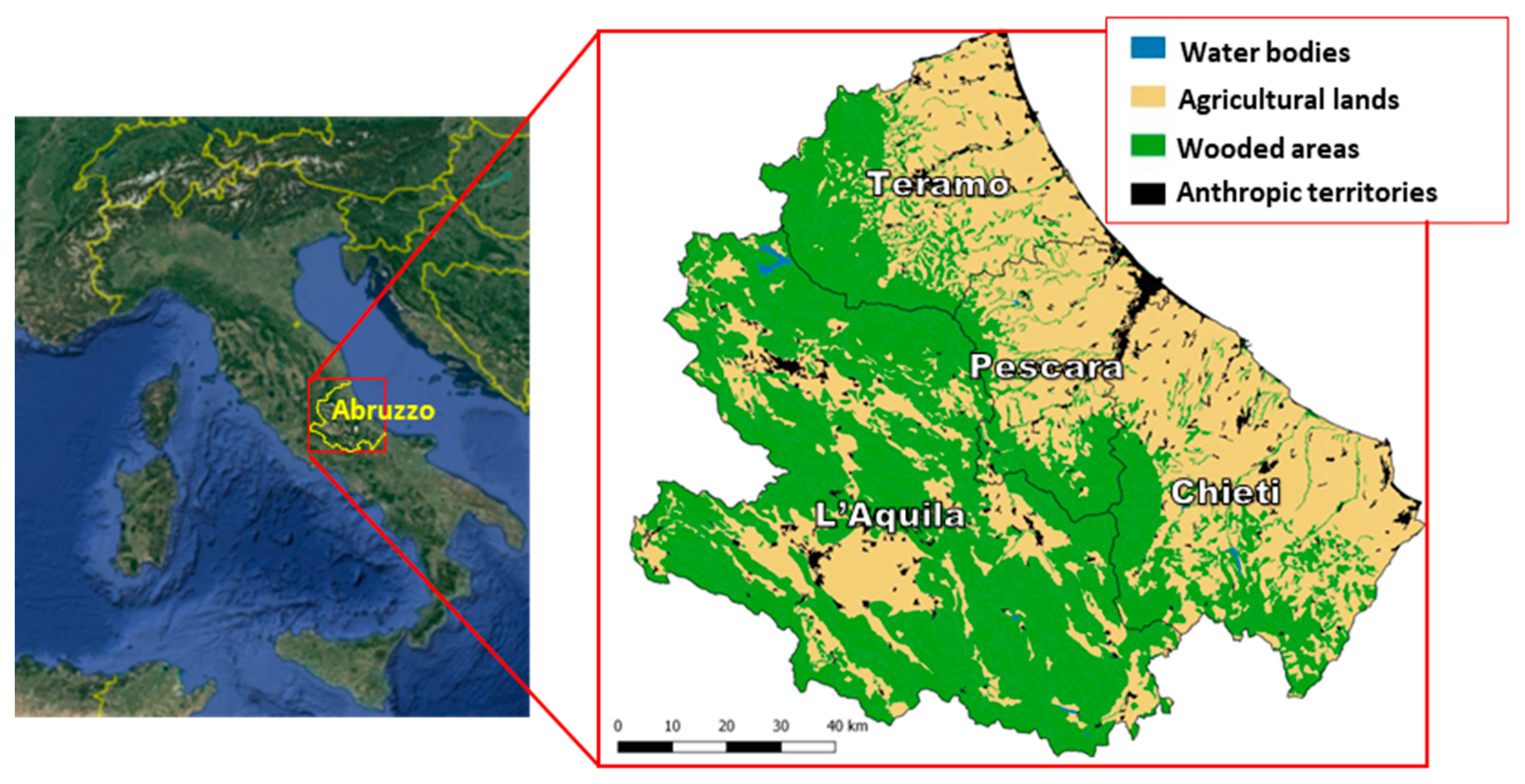
2. The Study Area
2.1. Main Geographic and Climatic Features
- The internal belt (mountainous) characterized by a complex orography and exhibiting extensive high-altitude areas, such as mountains, basins, and valleys. This zone experiences various microclimates, with a prevailing semi-continental climate, featuring hot summers and cold winters;
- The eastern belt (hilly and coastal) characterized by a more uniform and typically Mediterranean climate, with hot summers and mild winters.
2.2. Agricultural Activity in the Abruzzo Region
3. Data and Methods
3.1. Climatic Data
- The short-term SPI/SPEI (1 to 3 months) indicates immediate impacts on soil moisture, snow cover and flow rate in small streams;
- The medium-term SPI/SPEI (3 to 6 months) assesses reductions in river flows and the crop production yield;
- The long-term SPI/SPEI (6 to 12 months) reveals changes in reservoir capacities and river flows;
- The very long-term SPI/SPEI (over 12 months) assesses the reduced recharge of reservoirs and large water basins and the availability of water in aquifers.
3.2. Trend Analysis
3.3. Climatic Classifications
3.4. Agricultural Data
- (1)
- The harvested area and production (Figure 2) values for all crops in Abruzzo were sorted in descending order for the years 1952 and 2018;
- (2)
- Only crops that covered at least 75% of the total harvested area and accounted for at least the same percentage of the total production were considered;
- (3)
- Crops that were present in only one of the two reference years were excluded to avoid those crops that were cultivated only in the past or that have been introduced recently.
3.5. Correlation Analysis between Crop Yields and Drought Indices
4. Results
4.1. Climatic Analysis
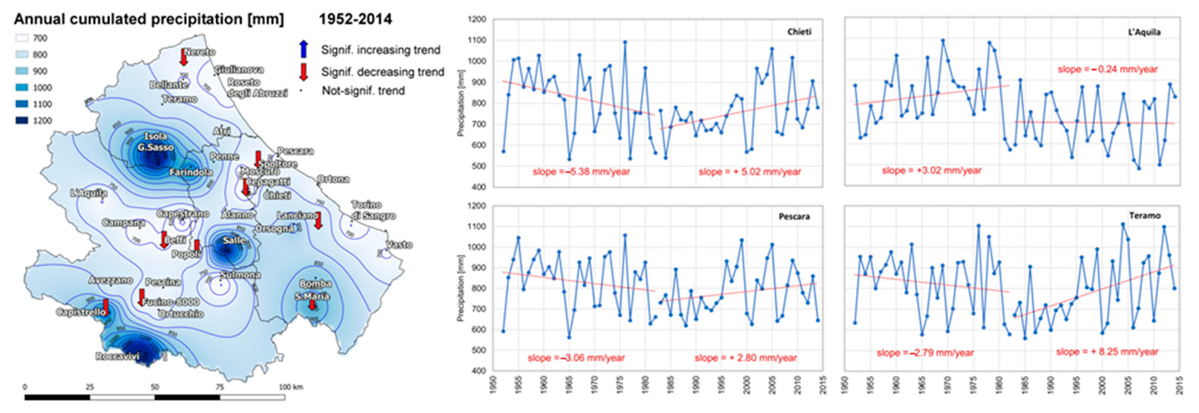
4.1.1. Precipitation Trend Analysis
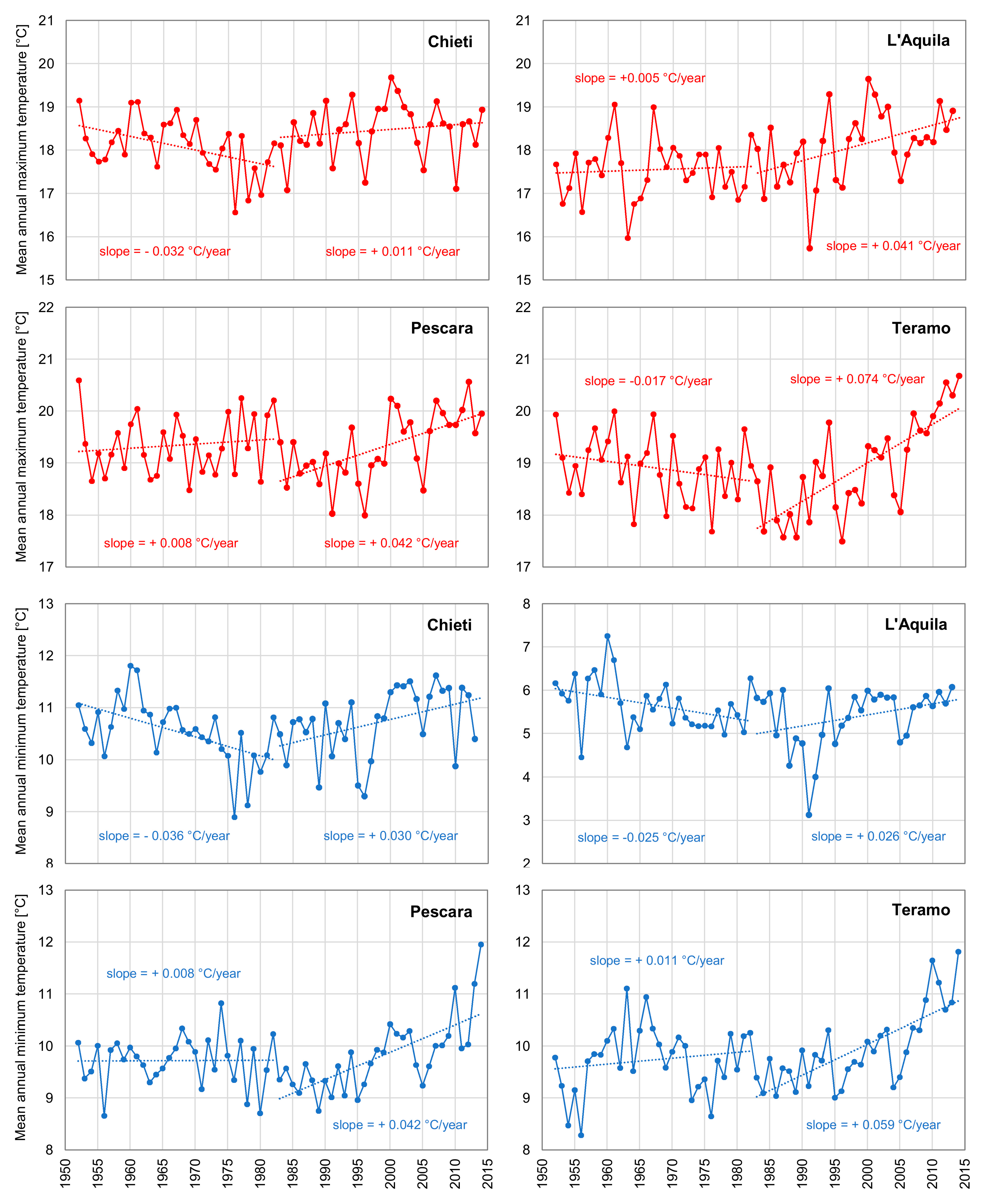
4.1.2. Temperature Trend Analysis
4.1.3. Climatic Classification
- In the province of Chieti, in July and August, it transitioned from having temperate or borderline conditions to arid during the second three decades. This shift resulted from elevated average temperatures coupled with decreased rainfall;
- In the province of L’Aquila, in July and August, it shifted to arid conditions in the later three decades due to increased temperatures. Conversely, in February and November, with stable average temperatures, the region experienced diminished precipitation, leading to a more temperate climate. A substantial reduction in rainfall exceeding 30 mm is evident in January and December during the latter period.
- In the province of Pescara, the overall climograph remained relatively consistent, except for July and August, during which it shifted from warm to dry due to decreased precipitation.
- In the province of Teramo, July and August persisted as warm months, while January transitioned to the temperate category due to increased temperatures and reduced rainfall.
4.1.4. Drought Indices
4.2. Agricultural Yield Data
4.3. Correlation Analysis of Crop Yields and Drought Indices
- Correlation sign: positive correlations are represented by blue (dark or light) filled squares, while negative correlations are denoted by red squares.
- Correlation significance: the statistical significance of the correlation was checked using the two-tailed Student’s t-test at the 10% and 1% significance levels, which are associated with the threshold correlation values (see the legend in Figure 10).
5. Discussion
6. Perspective for Future Research
7. Conclusions
- Over the two considered time periods, the region’s climatic classification has undergone a transformation, with a shift towards more temperate conditions in the winter months and a transition to warmer and more arid climate during the summer season;
- SPI and SPEI drought indices point out an increase in drought intensity and persistence, starting from the 1980s;
- In contrast to 1952–1982, the period 1983–2014 exhibited a distinct rise in the correlation magnitude between the crop yields and climatic drought indices. Despite the progressive improvements in the agricultural production system, this shift should be interpreted as a sign of its increasing sensitivity to climate stresses.
Author Contributions
Funding
Institutional Review Board Statement
Informed Consent Statement
Data Availability Statement
Acknowledgments
Conflicts of Interest
References
- IPCC. Summary for Policymakers. In Climate Change 2021: The Physical Science Basis; Contribution of Working Group I to the Sixth Assessment Report of the Intergovernmental Panel on Climate Change; Masson-Delmotte, V., Zhai, P., Pirani, A., Connors, S.L., Péan, C., Berger, S., Caud, N., Chen, Y., Goldfarb, L., Gomis, M.I., et al., Eds.; Cambridge University Press: Cambridge, UK, 2021. [Google Scholar]
- Abbass, K.; Qasim, M.Z.; Song, H.; Murshed, M.; Mahmood, H.; Younis, I. A review of the global climate change impacts, adaptation, and sustainable mitigation measures. Environ. Sci. Pollut. Res. 2022, 29, 42539–42559. [Google Scholar] [CrossRef] [PubMed]
- Nguyen, P.; Thorstensen, A.; Sorooshian, S.; Hsu, K.; Ashouri, H.; Tran, H.; Braithwaite, D.; AghaKouchak, A. Global Precipitation Trends across Spatial Scales Using Satellite Observations. Bull. Am. Meteorol. Soc. 2018, 99, 689–697. [Google Scholar] [CrossRef]
- Giorgi, F.; Lionello, P. Climate change projections for the Mediterranean region. Glob. Planet. Change 2008, 63, 90–104. [Google Scholar] [CrossRef]
- Michaelides, S.; Karacostas, T.; Sánchez, J.L.; Retalis, A.; Pytharoulis, I.; Homar, V.; Romero, R.; Zanis, P.; Giannakopoulos, C.; Bühl, J.; et al. Reviews and perspectives of high impact atmospheric processes in the Mediterranean. Atmos. Res. 2018, 208, 4–44. [Google Scholar] [CrossRef]
- Tuel, A.; Eltahir, E.A. Why is the Mediterranean a climate change hot spot? J. Clim. 2020, 33, 5829–5843. [Google Scholar] [CrossRef]
- Fioravanti, G.; Piervitali, E.; Desiato, F. A new homogenized daily data set for temperature variability assessment in Italy. Int. J. Clim. 2019, 39, 5635–5654. [Google Scholar] [CrossRef]
- Scorzini, A.R.; Leopardi, M. Precipitation and temperature trends over central Italy (Abruzzo Region): 1951–2012. Theor. Appl. Clim. 2018, 135, 959–977. [Google Scholar] [CrossRef]
- Caporali, E.; Lompi, M.; Pacetti, T.; Chiarello, V.; Fatichi, S. A review of studies on observed precipitation trends in Italy. Int. J. Climatol. 2021, 41, E1–E25. [Google Scholar] [CrossRef]
- Curci, G.; Guijarro, J.A.; Di Antonio, L.; Di Bacco, M.; Di Lena, B.; Scorzini, A.R. Building a local climate reference dataset: Application to the Abruzzo region (Central Italy), 1930–2019. Int. J. Clim. 2021, 41, 4414–4436. [Google Scholar] [CrossRef]
- Aruffo, E.; Di Carlo, P. Homogenization of instrumental time series of air temperature in Central Italy (1930-2015). Clim. Res. 2019, 77, 193–204. [Google Scholar] [CrossRef]
- Spinoni, J.; Vogt, J.V.; Naumann, G.; Barbosa, P.; Dosio, A. Will drought events become more frequent and severe in Europe? Int. J. Climatol. 2018, 38, 1718–1736. [Google Scholar] [CrossRef]
- McKee, T.B.; Doesken, N.J.; Kleist, J. The relationship of drought frequency and duration to time scales. In Proceedings of the 8th Conference on Applied Climatology, Anaheim, CA, USA, 17–22 January 1993; Volume 17, No. 22. pp. 179–183. [Google Scholar]
- Vicente-Serrano, S.M.; Beguería, S.; López-Moreno, J.I. A Multiscalar Drought Index Sensitive to Global Warming: The Standardized Precipitation Evapotranspiration Index. J. Clim. 2010, 23, 1696–1718. [Google Scholar] [CrossRef]
- Palmer, W.C. Meteorological Drought; US Department of Commerce, Weather Bureau: Washington, DC, USA, 1965; Volume 30.
- Narasimhan, B.; Srinivasan, R. Development and evaluation of Soil Moisture Deficit Index (SMDI) and Evapotranspiration Deficit Index (ETDI) for agricultural drought monitoring. Agric. For. Meteorol. 2005, 133, 69–88. [Google Scholar] [CrossRef]
- World Meteorological Organization (WMO); Global Water Partnership (GWP). Handbook of Drought Indicators and Indices; Svoboda, M., Fuchs, B.A., Eds.; Integrated Drought Management Programme (IDMP), Integrated Drought Management Tools and Guidelines Series 2; World Meteorological Organization (WMO) and Global Water Partnership (GWP): Geneva, Switzerland, 2016; ISBN 978-92-63-11173-9. [Google Scholar]
- Potopová, V.; Boroneanţ, C.; Boincean, B.; Soukup, J. Impact of agricultural drought on main crop yields in the Republic of Moldova. Int. J. Clim. 2016, 36, 2063–2082. [Google Scholar] [CrossRef]
- Bezdan, J.; Bezdan, A.; Blagojević, B.; Mesaroš, M.; Pejić, B.; Vranešević, M.; Pavić, D.; Nikolić-Đorić, E. SPEI-Based Approach to Agricultural Drought Monitoring in Vojvodina Region. Water 2019, 11, 1481. [Google Scholar] [CrossRef]
- Gunst, L.; Rego, F.M.C.C.; Dias, S.M.A.; Bifulco, C.; Stagge, J.H.; Rocha, M.S.; Van Lanen, H.A.J. Links between Meteorological Drought Indices and Yields (1979–2009) of the Main European Crops; Technical Report No. 36; DROUGHT-R&SPI Project: Wageningen, The Netherlands, 2015. [Google Scholar]
- Peña-Gallardo, M.; Vicente-Serrano, S.M.; Domínguez-Castro, F.; Beguería, S. The impact of drought on the productivity of two rainfed crops in Spain. Nat. Hazards Earth Syst. Sci. 2019, 19, 1215–1234. [Google Scholar] [CrossRef]
- Peña-Gallardo, M.; Vicente-Serrano, S.M.; Domínguez-Castro, F.; Quiring, S.; Svoboda, M.; Beguería, S.; Hannaford, J. Effectiveness of drought indices in identifying impacts on major crops across the USA. Clim. Res. 2018, 75, 221–240. [Google Scholar] [CrossRef]
- Blauhut, V.; Gudmundsson, L.; Stahl, K. Towards pan-European drought risk maps: Quantifying the link between drought indices and reported drought impacts. Environ. Res. Lett. 2015, 10, 014008. [Google Scholar] [CrossRef]
- Bachmair, S.; Tanguy, M.; Hannaford, J.; Stahl, K. How well do meteorological indicators represent agricultural and forest drought across Europe? Environ. Res. Lett. 2018, 13, 034042. [Google Scholar] [CrossRef]
- Labudová, L.; Labuda, M.; Takáč, J. Comparison of SPI and SPEI applicability for drought impact assessment on crop production in the Danubian Lowland and the East Slovakian Lowland. Theor. Appl. Climatol. 2017, 128, 491–506. [Google Scholar] [CrossRef]
- Martinez, C.J.; Baigorria, G.A.; Jones, J.W. Use of climate indices to predict corn yields in southeast USA. Int. J. Clim. 2009, 29, 1680–1691. [Google Scholar] [CrossRef]
- Parsons, D.J.; Rey, D.; Tanguy, M.; Holman, I.P. Regional variations in the link between drought indices and reported agricultural impacts of drought. Agric. Syst. 2019, 173, 119–129. [Google Scholar] [CrossRef]
- Chen, T.; Xia, G.; Liu, T.; Chen, W.; Chi, D. Assessment of Drought Impact on Main Cereal Crops Using a Standardized Precipitation Evapotranspiration Index in Liaoning Province, China. Sustainability 2016, 8, 1069. [Google Scholar] [CrossRef]
- Tian, L.; Yuan, S.; Quiring, S.M. Evaluation of six indices for monitoring agricultural drought in the south-central United States. Agric. For. Meteorol. 2018, 249, 107–119. [Google Scholar] [CrossRef]
- Di Lena, B.; Farinelli, D.; Palliotti, A.; Poni, S.; DeJong, T.M.; Tombesi, S. Impact of climate change on the possible expansion of almond cultivation area pole-ward: A case study of Abruzzo, Italy. J. Hortic. Sci. Biotechnol. 2018, 93, 209–215. [Google Scholar] [CrossRef]
- Di Lena, B.; Curci, G.; Vergni, L.; Farinelli, D. Climatic Suitability of Different Areas in Abruzzo, Central Italy, for the Cultivation of Hazelnut. Horticulturae 2022, 8, 580. [Google Scholar] [CrossRef]
- Di Carlo, P.; Aruffo, E.; Brune, W.H. Precipitation intensity under a warming climate is threatening some Italian premium wines. Sci. Total Environ. 2019, 685, 508–513. [Google Scholar] [CrossRef]
- Giraudi, C.; Magny, M.; Zanchetta, G. Drysdale the Holocene climatic evolution of Mediterranean Italy: A review of the continental geological data. Holocene 2011, 21, 105–115. [Google Scholar] [CrossRef]
- Cosentino, D.; Cipollari, P.; Marsili, P.; Scrocca, D. Geology of the central Apennines: A regional review. In The Geology of Italy: Tectonics and Life along Plate Margins; Beltrando, M., Peccerillo, A., Mattei, M., Conticelli, S., Doglioni, C., Eds.; Journal of the Virtual Explorer, Electronic Edition; 2010; Volume 36, p. 11. ISSN 1441-8142. [Google Scholar] [CrossRef]
- Cosentino, D.; Asti, R.; Nocentini, M.; Gliozzi, E.; Kotsakis, T.; Mattei, M.; Esu, D.; Spadi, M.; Tallini, M.; Cifelli, F.; et al. New insights into the onset and evolution of the central Apennine extensional intermontane basins based on the tectonically active L’Aquila Basin (central Italy). Bull. Geol. Soc. Am. 2017, 129, 1314–1336. [Google Scholar] [CrossRef]
- Zucaro, R.; Pontrandolfi, A. Rapporto Sullo Stato dell’Irrigazione in Abruzzo; Istituto Nazionale di Economia Agraria INEA: Rome, Italy, 2008. Available online: https://sigrian.crea.gov.it/wp-content/uploads/2020/11/2008-Rapporto-sullo-stato-dellirrigazione-in-Abruzzo.pdf (accessed on 15 August 2023).
- Piacentini, T.; Buccolini, M.; Miccadei, E. The Terminillo, Gran Sasso and Majella Mountains: The ‘Old Guardians’ of the Tyrrhenian and Adriatic Seas. In Landscapes and Landforms of Italy. World Geomorphological Landscapes; Soldati, M., Marchetti, M., Eds.; Springer: Cham, Switzerland, 2017. [Google Scholar]
- Santo, A.; Ascione, A.; Di Crescenzo, G.; Miccadei, E.; Piacentini, T.; Valente, E. Tectonic-geomorphological map of the middle Aterno river valley (Abruzzo, Central Italy). J. Maps 2014, 10, 365–378. [Google Scholar] [CrossRef]
- Regione Abruzzo, 2014. Sviluppo Rurale in Abruzzo nel 2014–2020. Available online: https://rica.crea.gov.it/APP/PSR_2014_2020/download/04_AnalisiDiContesto.pdf (accessed on 10 July 2023).
- ISTAT, Biblioteca Digitale-Annuario di Statistica Agraria. Available online: https://ebiblio.istat.it/SebinaOpac/resource/annuario-di-statistica-agraria/IST0010796 (accessed on 15 August 2023).
- ISTAT, Dati-Agricoltura-Coltivazioni-Superfici e Produzione. Available online: http://dati.istat.it (accessed on 15 August 2023).
- Annali Idrologici della Regione Abruzzo, Ufficio Idrografico e Mareografico—Pescara. Available online: https://www.regione.abruzzo.it/content/annali-idrologici?page=2 (accessed on 15 August 2023).
- Annali Idrologici della Regione Campania, Centro Funzionale Multirischi della Protezione Civile Regione Campania, Annali Idrologici e Altre Pubblicazioni del Compartimento di Napoli del S.I.M.N. Available online: http://centrofunzionale.regione.campania.it/#/pages/documenti/annali (accessed on 15 August 2023).
- Scorzini, A.R.; Di Bacco, M.; Leopardi, M. Recent trends in daily temperature extremes over the central Adriatic region of Italy in a Mediterranean climatic context. Int. J. Clim. 2018, 38, e741–e757. [Google Scholar] [CrossRef]
- Thornthwaite, C.W. An Approach toward a Rational Classification of Climate. Geogr. Rev. 1948, 38, 55–94. [Google Scholar] [CrossRef]
- Beguería, S.; Vicente-Serrano, S.M.; Reig, F.; Latorre, B. Standardized precipitation evapotranspiration index (SPEI) revisited: Parameter fitting, evapotranspiration models, tools, datasets and drought monitoring. Int. J. Climatol. 2014, 34, 3001–3023. [Google Scholar] [CrossRef]
- Mann, H.B. Non-Parametric Test against Trend. Econometrica 1945, 13, 245–259. [Google Scholar] [CrossRef]
- Kendall, M.G. Rank Correlation Methods, 4th ed.; Charles Griffin: London, UK, 1975. [Google Scholar]
- Sen, P.K. On a Further Robustness Property of the Test and Estimator Based on Wilcoxon’s Signed Rank Statistic. Ann. Math. Stat. 1968, 39, 282–285. [Google Scholar] [CrossRef]
- Di Lena, B.; Antenucci, F.; Mariani, L. Space and time evolution of the Abruzzo precipitation. Ital. J. Agrometeorol. 2012, 1, 5–20. [Google Scholar]
- Klein Tank, A.M.G.; Wijngaard, J.B.; Können, G.P.; Böhm, R.; Demarée, G.; Gocheva, A.; Mileta, M.; Pashiardis, S.; Hejkrlik, L.; Kern-Hansen, C.; et al. Daily dataset of 20th-century surface air temperature and precipitation series for the European Climate Assessment. Int. J. Climatol. 2002, 22, 1441–1453. [Google Scholar] [CrossRef]
- Jones, P.D.; Moberg, A. Hemispheric and Large-Scale Surface Air Temperature Variations: An Extensive Revision and an Update to 2001. J. Clim. 2003, 16, 206–223. [Google Scholar] [CrossRef]
- Péguy, C.P. Précis de Climatologie, 2nd ed.; Masson: Paris, France, 1970; 468p. [Google Scholar]
- Ding, J.; Huang, Z.; Zhu, M.; Li, C.; Zhu, X.; Guo, W. Does cyclic water stress damage wheat yield more than a single stress? PLoS ONE 2018, 13, e0195535. [Google Scholar] [CrossRef]
- Orlandi, F.; Rojo, J.; Picornell, A.; Oteros, J.; Pérez-Badia, R.; Fornaciari, M. Impact of Climate Change on Olive Crop Production in Italy. Atmosphere 2020, 11, 595. [Google Scholar] [CrossRef]
- Rojo, J.; Salido, P.; Pérez-Badia, R. Flower and pollen production in the ‘Cornicabra’olive (Olea europaea L.) cultivar and the influence of environmental factors. Trees 2015, 29, 1235–1245. [Google Scholar] [CrossRef]
- Teslić, N.; Zinzani, G.; Parpinello, G.P.; Versari, A. Climate change trends, grape production, and potential alcohol concentration in wine from the “Romagna Sangiovese” appellation area (Italy). Theor. Appl. Climatol. 2018, 131, 793–803. [Google Scholar] [CrossRef]


| SPEI | |||||
|---|---|---|---|---|---|
| 1952–1982 | 1983–2014 | ||||
| + | − | + | − | ||
| Min. temp. | + | 29 | 29 | 19 | 30 |
| − | 26 | 16 | 22 | 30 | |
Disclaimer/Publisher’s Note: The statements, opinions and data contained in all publications are solely those of the individual author(s) and contributor(s) and not of MDPI and/or the editor(s). MDPI and/or the editor(s) disclaim responsibility for any injury to people or property resulting from any ideas, methods, instructions or products referred to in the content. |
© 2023 by the authors. Licensee MDPI, Basel, Switzerland. This article is an open access article distributed under the terms and conditions of the Creative Commons Attribution (CC BY) license (https://creativecommons.org/licenses/by/4.0/).
Share and Cite
Guerriero, V.; Scorzini, A.R.; Di Lena, B.; Iulianella, S.; Di Bacco, M.; Tallini, M. Impact of Climate Change on Crop Yields: Insights from the Abruzzo Region, Central Italy. Sustainability 2023, 15, 14235. https://doi.org/10.3390/su151914235
Guerriero V, Scorzini AR, Di Lena B, Iulianella S, Di Bacco M, Tallini M. Impact of Climate Change on Crop Yields: Insights from the Abruzzo Region, Central Italy. Sustainability. 2023; 15(19):14235. https://doi.org/10.3390/su151914235
Chicago/Turabian StyleGuerriero, Vincenzo, Anna Rita Scorzini, Bruno Di Lena, Stefano Iulianella, Mario Di Bacco, and Marco Tallini. 2023. "Impact of Climate Change on Crop Yields: Insights from the Abruzzo Region, Central Italy" Sustainability 15, no. 19: 14235. https://doi.org/10.3390/su151914235