1. Introduction
In a general context, the term permeability is a characteristic given to a material indicating the ease of flow of a fluid through such material [
1]. In petroleum engineering, it is known as the ability of porous rocks to pass through oil and/or gas [
2,
3,
4,
5]. Notably, it is not always necessary for a porous rock to be permeable. For a rock to be permeable and for the oil and/or gas to penetrate through it, the pore spaces between the grains in the relevant rock must be connected. This implies that permeability is a measure of the ability of oil and/or gas to penetrate through a rock [
6]. In this regard, one of the most widely used classification systems for carbonate rock porosity by petroleum geologists was introduced by Choquette and Pray in 1970 [
7]. This classification nomenclature is available in numerous books published on carbonate classification, for instance, Tucker and Wright (1990) [
8]. It has been cited as a main system for classifying porosity in carbonates.
Permeability is an essential reservoir property and a basic element of reservoir characteristics and the simulation process. This input is generally used to determine hydrocarbon production, recovery estimates, optimal well location, pressure, fluid contact classification, and so forth. More accurate predictions of reservoir permeability surely improve the overall exploration and discovery processes in the concerned area. Studies in the literature reveal that a more accurate prediction of coreless reservoir penetration is still a challenge in the oil and gas industry and needs significant concentration [
3,
4,
5]. It is also known that an accurate estimation of the permeability rate of a target reservoir is essential for the probable oil and gas repository in that reservoir [
2,
3,
4,
5,
9]. It may help in assessing the realistically achievable percentage of oil and gas, flow rate, estimation of future exploration, and the appropriate and correct design of exploration equipment.
Though permeability seems easy to realize, there exist several variables that may affect it, for example, the dynamic viscosity of the fluid, applied pressure difference, and rock/reservoir properties, such as grain size, sorting, and the pore’s throats [
10,
11]. Permeability can be measured in many ways [
10,
11]. In the beginning, it was primarily measured involving numerous parameters, such as the gamma-ray, neutron porosity, bulk density, resistance, sonic waves, spontaneous potential, well size, and/or reservoir depth. However, a standard method for determining permeability is performed using conventional core analysis (CCA) and/or the porosity permeability-relationship (PPR) while determining a non-linear relationship between porosity and permeability [
11]. Though traditional well testing, core analysis, and well-log evaluation can predict the permeability of carbonate reservoirs, these conventional methods are not only costly but also time-consuming. This is because the relevant persons make multiple visits to the laboratory to test target samples and predict permeability [
12]. In addition, estimating permeability in heterogeneous carbonate reservoirs are also a great challenge, which must be handled carefully to guarantee precise prediction [
10,
11]. As stated earlier, the permeability of a material is its capacity to allow fluids to flow through it. It is measured in the Darcy/Square-meter (Darcy/m
2), which is defined as the volume of fluid passing through a surface in the unit time under the surface pressure gradient at the point where flow passes through it [
1].
ML has inevitably been used in permeability prediction and found quite promising. For instance, a study conducted in [
13] employed white-box ML approach to model permeability from heterogeneous carbonate reservoirs in Iran. The algorithms are k-nearest neighbors (kNN), genetic programming (GP), and modified group modeling data handling (GMDH). The proposed study outperformed zone-specific permeability, index-based empirical, or data-driven models already investigated in the literature with R
2 values of 0.99 and 0.95 against GMDH and GP, respectively [
13]. The study was organized motivated by a study by the same authors in [
14], where they employed a supervised machine learning algorithm known as Extreme Gradient Boosting (XGB) on heterogeneous reservoir data to predict permeability. The output of the algorithm is a modified formation zone index (FZIM*), based on which the permeability was estimated as R
2 values of 0.97. The study further investigated the k-mean clustering algorithm to classify/categorize petrophysical rock typing (PRT) to study their properties.
Machine learning is a subfield of computer science and artificial intelligence that focuses on the development of algorithms that enable computers to learn from and make decisions or predictions based on data [
15]. The main objective is to model the probable relationship between a set of observable quantities (inputs) and another set of variables related to them (outputs) [
16]. Usually, all ML algorithms require large amounts of data for training and learning. This implies that collecting many of the representative training examples and saving them in a format suitable for computational purposes is an essential step [
16]. In general, target data are not ready to use because they may contain irrelevant attributes, missing attributes, redundant attributes, attribute-value noise, and class-label noise. The observable quantities that are usually fed to ML algorithms are called “features”. During training, a target algorithm struggles to learn to associate these features with the desired output variables, thereby fitting the model’s parameters. This implies that features must be relevant to predict outcomes with precision [
16]. This implies that pre-processing target data is an indispensable task. In this regard, several preprocessing techniques have been developed in the literature to handle various types of data. These include images, audio, text, video, and their combination. Accordingly, various techniques have been utilized to eliminate noisy and unwanted data [
16]. For instance, handling missing values, normalization for numeric data and scaling, filtering, and denoising are commonly used in images [
16].
The current study aims to develop an ensemble machine learning model for permeability prediction based on a diverse real-life dataset collected from a renowned, Middle Eastern company. Contributions of the proposed work are, firstly, conducting a literature review in permeability detection in carbonate reservoirs using machine learning techniques and finding a potential research gap. Second, based on the literature review, it was evident that machine learning has been frequently utilized; however, ensemble learning methods have yet to be investigated for the said problem, which is the aim of the study. Third, various preprocessing techniques have been employed to the real-life dataset prior to fetching it to the model and finally evaluating the model based on the well-known metrics used in the literature and contrasting the findings.
The rest of this paper is organized as follows.
Section 2 is centered around the related work. It briefly describes the ML model’s enhancement techniques, e.g., feature selection and ensemble techniques.
Section 3 elaborates the ML algorithms used in this study.
Section 4 describes the target oil well dataset. In addition, it details the experimental setup and subsequent experimentations.
Section 5 discusses the experimental setup and
Section 6 provides results and discussion. Lastly,
Section 7 concludes this study and provides future recommendations.
5. Experimental Setup
In this study, the proposed algorithm was implemented, validated, and tested in Python 3.10.4 (Jupyter). Since the OWL dataset possesses large and small values in the same records, the OWL datasets were normalized to ensure all data fall within the same range. However, this act does not affect the model’s judgment. The target OWL datasets are divided into nonoverlapping training and testing sets in a ratio of 8:2, respectively. Moreover, the authors applied cross-validation using the k-fold technique with five folds for each OWL.
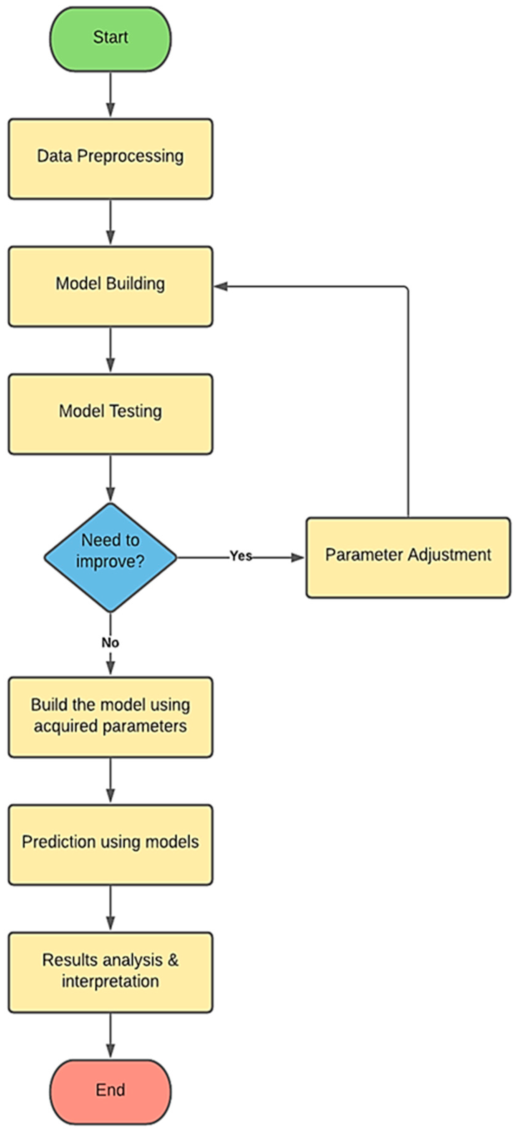
Furthermore, training data were used to create the models and test the models’ predictability. If a model still needed refinement after testing, the model’s hyperparameters were adjusted until optimum results were achieved. In this way, feature selection was conducted to improve performance [
34]. Finally, once satisfactory test results were obtained, the model was created using the obtained optimized hyperparameters. For instance, the parameters for the RF model (n_estimators = 100, random_state = 10); for AdaBoost (n_estemators = 30, Learning rate = 1, loss = ‘linear’, Random_state = 142) and for GB ((n_estemators = 100, Learning rate = 1, Random_state = 142) were used. After the model was validated, new data were used to make predictions. Predictions’ results were then analyzed and compared to identify the most effective model for RMSE value and other metrics.
Figure 1 shows the main phases of developing the machine learning prediction models.
5.1. Evaluation Criteria
This section elaborates the metrics utilized to measure the performance of the proposed scheme [
35,
36,
37,
38].
5.1.1. Root Mean-Squared Error (RMSE)
The
RMSE is a primary statistical measurement that is often used to assess a regression ML model while deciding its performance. It is calculated by taking the mean of the square of difference of the value predicted by the model and the actual value of the target sample. It is given in Equation (2).
where
n is the size of the dataset (number of instances).
5.1.2. Mean Absolute Error (MAE)
The MAE is also a statistical measurement used to assess a model’s performance. It shows the difference between every predicted value and its corresponding actual target value. In addition, a relative error is calculated as the ratio of mean of absolute values of error and mean value of predicted target value as given in Equation (3):
5.1.3. Coefficient of Determination (R2)
The
is a statistical measure in which an independent variable or variable(s) explains the variance of a dependent variable in a regression model.
explains how much variance in one variable explains variance in another, while correlation explains the strength of the relationship between one independent variable and another independent one, e.g., velocity (dependent) and time (independent). The formula for calculating the correlation coefficient is given in Equation (4) [
39,
40]:
The coefficient of determination is the square of the correlation coefficient.
6. Results and Discussion
All experiments were performed using the following:
Training models using the whole dataset obtained from exploration fields.
Training models after applying the pre-processing steps on the dataset.
Results of testing are presented rather than training, which is more realistic because the test data is distinct.
As stated earlier, all data samples were first normalized, and then outliers were removed using the standard deviation-based method. Relevant features were selected based on their correlation with the target attribute, i.e., permeability. The measure of performance was done by monitoring three major measurements: R
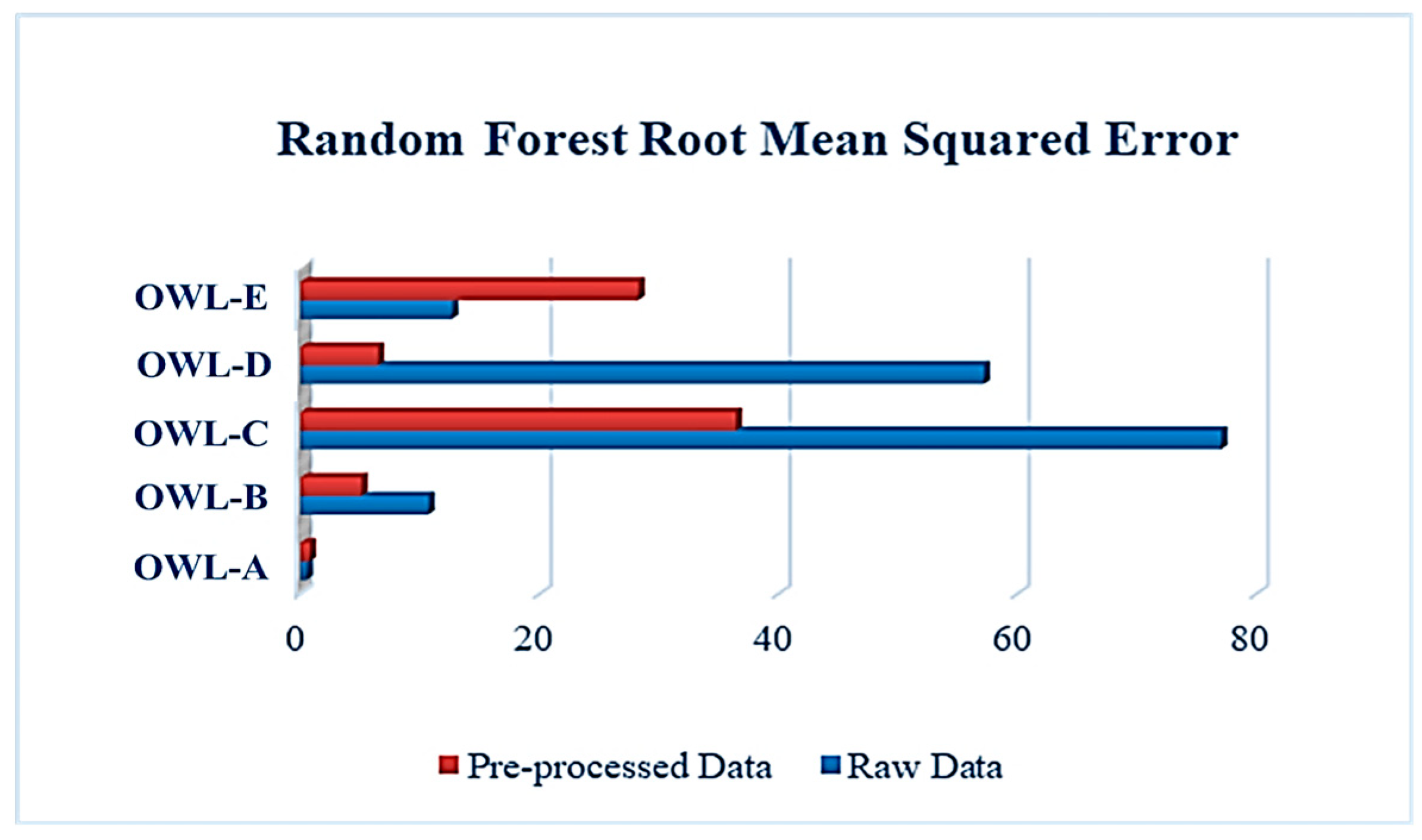
2, RMSE, and MAE. These metrics represent the coefficient of correlation, root mean squared error, and mean absolute error, respectively. As for the correlation coefficient, the higher its value, the better the model’s performance. This is the opposite for the RMSE and MAE, measuring the error of the model’s performance. Thus, the lower the value of RMSE and MAE, the better the model’s performance would be. From
Figure 2, it can be inferred that the RF model performed marginally better when used with the pre-processed data for most OWL, with the RMSE value decreasing from 57.195 to 6.468 in OWL-D alone in addition to OWL-C. The value dropped from 77.054 to 36.422 and OWL-B went down from 10.697 to 5.087. These facts show that this improvement in performance is proof that the used pre-processing techniques were more effective and had a great impact on the model’s learning capability.
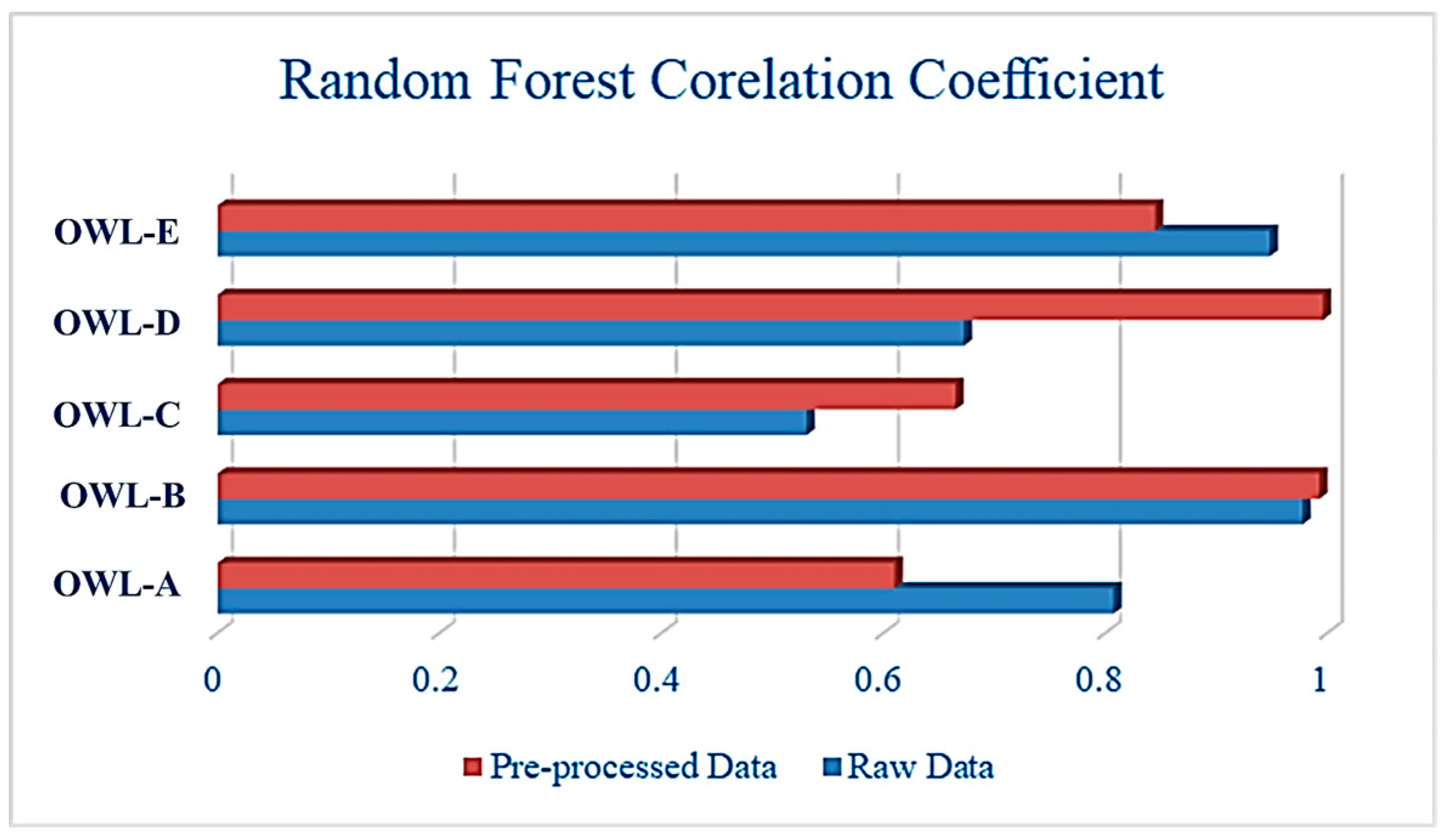
Figure 2 and
Figure 3 provide a comprehensive look into the performance of the raw and pre-processed data for the same model by means of RMSE and correlation coefficient.
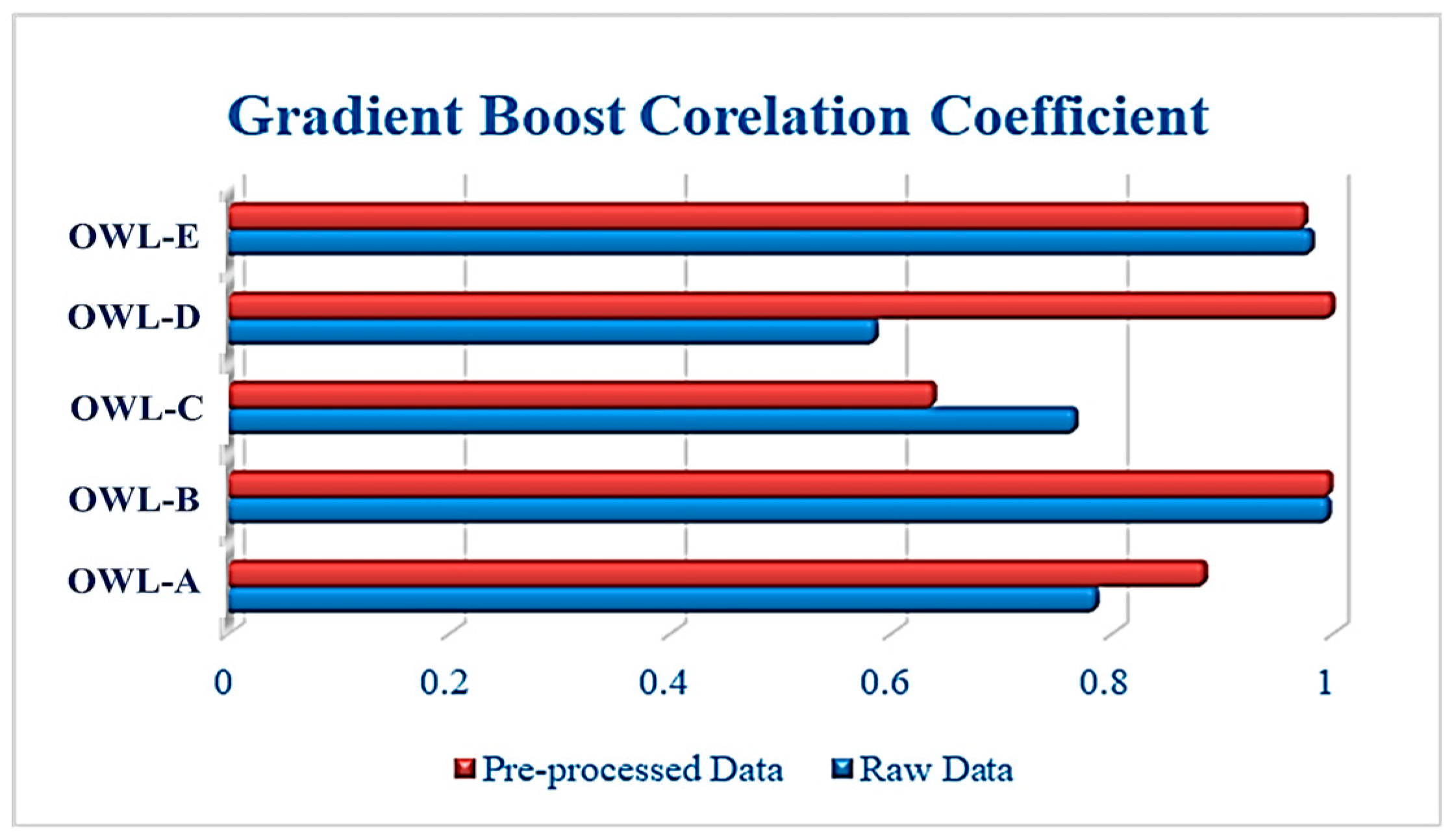
According to
Figure 4, the GB algorithm achieves the highest value of correlation coefficient at 99.8% for OWL-B for both raw and preprocessed data. This means that for this OWL, GB was robust against the raw data vulnerability. Similarly, it exhibited the same results for OWL-D but for preprocessed data only, while for its raw data counterpart its performance was below 60%. The main reason behind such differences is the nature of the data obtained from each well. For OWL-E again, the performance was remarkably good, as the value of correlation coefficients was 98.2% and 98% for raw and preprocessed data, respectively.
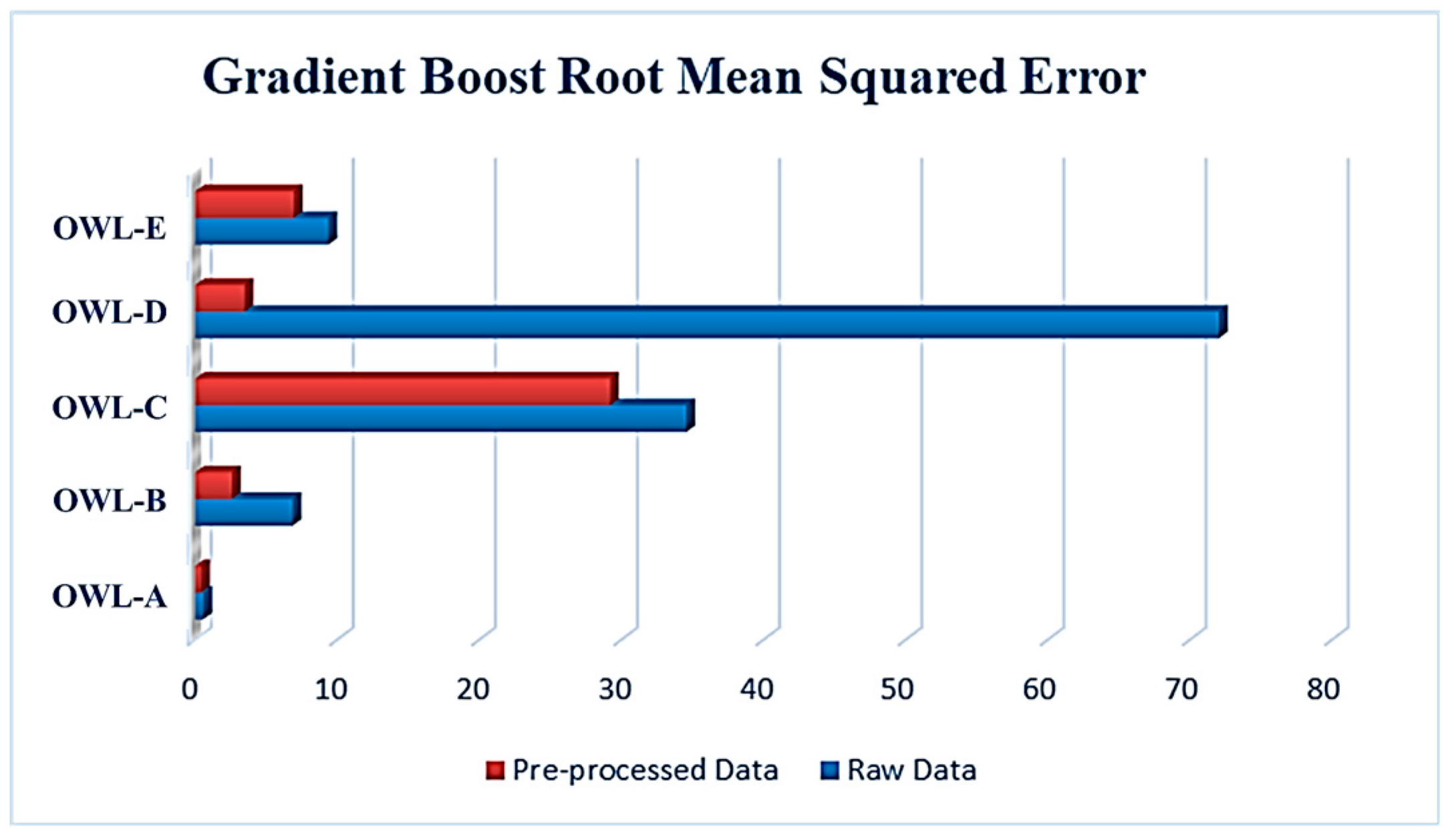
Figure 5 reports the RMSE analysis for the GB algorithm with and without preprocessed data. The results were quite interesting, as OWL-A with raw data significantly outperformed all other OWL with a negligible error, followed by OWL-B and OWL-E. Nonetheless, OWL-D with raw data exhibited an RMSE of 72. The effects of pre-processing techniques can be seen on all OWLs when using the gradient boost algorithm. The performance indicators clearly show this effect in
Figure 5. The value of the RMSE of OWL-D sharply decreased from 72.007 to 3.465. Furthermore, the RMSE values of OWL-C and OWL-E shrank from 34.55 and 9.367 to 29.177 and 6.931, respectively. For OWL-A, the RMSE decreased slightly from 0.57 to 0.398. This slight decrease in OWL-A’s value was expected because most of the models performed great with OWL-A in the first place.
Table 4 shows the RMSE values for each algorithm. It was concluded that the best performing algorithm was GB with an average RMSE value of 8.506, followed by RF with an average RMSE value of 15.399. In addition to the previously discussed algorithms (GB, RF), multiple algorithms were trained and tested on the same OWL dataset, preprocessing, and using the same experimental setup. These algorithms included AdaBoost, XGB, SVR, and LR. However, the results gained from these algorithms were not sufficient even after tuning their hyperparameters. These algorithms were excluded due to unsatisfying performance, supported by the fact that their performance measures showed fairly high RMSE and MAE values, as well as low values of correlation coefficient. Referring to
Table 4, it can be deduced that the average values of RMSE were between 16.965 and 97.6, which was a considerably high value compared to the performance of both GB and RF models. Though pre-processing techniques used in this project enhanced the performance of some ML models, a few models did not produce satisfying results, which may be caused by the nature of the data, or the nature of the algorithms being investigated.
6.1. Comparison with State-of-the-Art
The authors in [
10,
12] used the same OWL dataset to train, validate, and test their proposed models to predict permeability. They applied the SVM algorithm in [
10] and ANN in [
12]. When applied to the same OWL dataset, the proposed gradient boosting regressor scheme proved its superiority over the two algorithms mentioned above. It obtained a lower RMSE for all OWLs, except OWL-C.
Table 5 and
Table 6 offer a comparative analysis of these algorithms. Overall, the proposed scheme outperformed state-of-the-art techniques in the literature for the same dataset. One potential reason that GBR outperforms ANN is due to its nature that it is more suitable for the numeric datatype.
6.2. Limitations of the Study
As far as limitations of the study are concerned, firstly, there were five wells’ data with an unequal number of instances, and data were unbalanced. Some data balancing techniques, such as the synthetic minority oversampling technique (SMOTE), can be applied to balance the dataset prior to modeling. That can further fine-tune the results. Moreover, according to
Table 1, there is a slight difference in the number of attributes in each well.


 ,
, 


