Article

A Two-Stage Robust Optimization Microgrid Model Considering Carbon Trading and Demand Response

School of Economics and Management, Shanghai University of Electric Power, Shanghai 201306, China
*
Author to whom correspondence should be addressed.
Sustainability 2023, 15(19), 14592; https://doi.org/10.3390/su151914592
Submission received: 3 September 2023 / Revised: 28 September 2023 / Accepted: 7 October 2023 / Published: 8 October 2023

Abstract

:
To enhance the low-carbon level and economic performance of microgrid systems while considering the impact of renewable energy output uncertainty on system operation stability, this paper presents a robust optimization microgrid model based on carbon-trading mechanisms and demand–response mechanisms. Regarding the carbon-trading mechanism, the baseline allocation method is utilized to provide carbon emission quotas to the system at no cost, and a ladder carbon price model is implemented to construct a carbon transaction cost model. Regarding uncertainty set construction, the correlation of distributed generation in time and space is considered, and a new uncertainty set is constructed based on historical data to reduce the conservative type of robust optimization. Based on the column constraint generation algorithm, the model is solved. The findings indicate that upon considering the carbon-trading mechanism, the microgrid tends to increase the output of low-carbon units and renewable energy units, and the carbon emissions of the microgrid can be effectively reduced. However, due to the increase in power purchase from the distribution network and the increase in carbon transaction costs, the operating costs of the microgrid increase. Secondly, through the utilization of demand–response mechanisms, the microgrid can achieve load transfer between peaks and troughs. It is imperative to establish appropriate compensation costs for demand and response that balances both economic efficiency and system stability. At the same time, due to the time-of-use electricity price, the energy storage equipment can also play a load transfer effect and improve the system’s economy. Finally, sensitivity analysis was conducted on the adjustment parameters of distributed power sources and loads that have uncertain values. A comparison was made between the deterministic scheduling model and the two-stage robust optimization model proposed in this study. It was proved that this model has great advantages in coordinating the economy, stability and low carbon level of microgrid operations.

1. Introduction

As a signatory of the Paris Climate Agreement, the Chinese government has made significant strategic decisions tied to China’s sustainable development and the creation of a community with a shared future for mankind. The “dual-carbon goal” is a serious commitment made by China as a responsible global power to combat global climate change in line with China’s unique national circumstances [1]. It provides a solution with China’s unique features to facilitate the reform of the energy supply and consumption, upgrade traditional industries, and establish a low-carbon society [2]. Achieving the “double-carbon” goal will help solve recent extreme, bad weather problems and improve the quality of social life.
As the world’s second-largest economy, China has seen a consistent rise in its carbon emissions in recent years [3]. A significant proportion of these emissions, over 40%, can be attributed to the combustion of fossil fuels during power generation [4,5]. In recent years, carbon emission reduction targets have become more and more urgent. In order to control carbon emissions, it is essential to implement a carbon emissions trading (CET) system in the power sector. Day-ahead optimal scheduling is an integral part of decision-making for power system operations and is inevitably impacted by the carbon emission trading mechanism [6]. Consequently, there is significant theoretical and practical value in studying the day-ahead optimal scheduling method for power systems that incorporate carbon emission trading. Cui et al. [7] analyzed the effectiveness of the traditional CET mechanism and compared it to the stepped CET mechanism, highlighting the rationale behind incorporating the stepped carbon-trading mechanism into optimal power dispatching. Akulker et al. [8] explored the impact of the CET mechanism on the optimal equipment selection and size. Yan et al. [9] employed the baseline approach for assigning carbon emission allowances to the system in the absence of compensation, and optimized the scheduling plan.
To achieve the ‘double-carbon’ target, the energy structure needs to be optimized. Nevertheless, as the presence of renewable energy continues to increase, the uncertainty associated with its power generation may have significant implications for the secure and reliable operation of the electricity grid. Finding ways to enhance the integration of renewable energy while maintaining grid stability has become a pressing concern [10]. In this context, microgrids, as an autonomous unit integrating energy production, transmission, storage and consumption can provide a localized, community-based energy management method, which has attracted more and more attention [11,12]. Economic dispatch for microgrids is a salient topic in microgrid research. The optimization methods are divided into dynamic programming, mixed-integer programming, stochastic programming, nonlinear programming and integer programming [13]. For the uncertain factors in the microgrid, stochastic programming and scenario analysis are often used to model uncertain variables. Stochastic programming employs probabilistic variables to depict uncertain data and arrives at an optimal scheduling plan based on the least expected expenses. Based on the probability theory, the scenario analysis method describes the uncertain information of the research object in a scenario manner, and the obtained scheduling scheme needs to have good performance in different scenarios. Bahramara et al. [14] proposed a decision-making framework that guarantees the optimal scheduling of distributed energy resources while providing energy and reserves. The uncertainty is visualized by a risk-based stochastic method, and the risk in the decision-making of microgrid operators is controlled by the conditional risk value method. Hadayeghparast et al. [15] employed scenario-based modelling to account for uncertainties in wind speed, solar radiation, market prices, and power loads, ultimately implementing a two-stage stochastic program. Kong et al. [16] utilized chance constraint programming to address uncertainties in renewable energy and loads, optimizing the output of distributed generation with a focus on cost minimization. Furthermore, some scholars employ machine-learning techniques to optimize microgrids. Cao et al. [17] put forward an enhanced dual-archive multi-objective evolutionary algorithm to encourage coordination of microgrid economic stability. Jiang et al. [18] implemented the downlink risk constraint method to model multiple energy sources for energy hub risk. Zheng et al. [19] suggested the use of ant lion optimization to address power system stability issues. Deng et al. [20] introduced an adaptive power-sharing approach, utilizing neural networks, to decrease transmission loss and total power capacity.
Another solution to the uncertainties in the microgrid is to use a robust optimization algorithm. That algorithms only require the boundary of the uncertainty set, rather than an exact probability distribution, to ensure system reliability in worst-case scenarios. Dong et al. [21] utilized a clustering method to categorize historical small hydropower inflow scenarios into several typical scenarios. They then developed a two-stage stochastic robust optimization model to calculate final operating costs under worst-case wind power output scenarios. Naji et al. [22] proposed a new control algorithm and a flexible energy management system to optimize operating costs in hybrid microgrids. They established interrelationships among planning elements to achieve their goals. Lotfi et al. [23] proposed a robust model for microgrid planning, along with their strategy for modification. Wang et al. [24] considered the uncertainty of electricity price when constructing the uncertainty set, and reduced the conservatism of robust optimization results by adding budget parameters. Considering the influence of wind power fluctuation and frequency regulation ability, Li et al. [25] developed a two-stage robust optimization model utilizing fuzzy sets for wind power. In order to fully adapt to renewable energy and cope with the imbalance between supply and demand, previous studies have mainly focused on demand response (DR) or energy storage systems. The DR concept covers any intentional modification of the user’s use of electricity [26,27]. The DR can be achieved through load regulation and control, and is critical to improving performance and security [28]. Energy storage systems can promote renewable energy consumption and reduce total system costs [29]. Dashtdar et al. [30] solved the problem of optimal operation and demand side management of microgrids through a combination of genetic algorithms and artificial bee colony. AlDavood et al. [31] proposed a robust scheduling model for islanded microgrids considering demand response, which is solved using a hybrid method combining genetic algorithms and mixed-integer programming. Yu et al. [32] formulated an optimal scheduling model centred on DR, cooperative energy storage system operation, and relevant constraints.
The formulation of uncertainty sets has a direct impact on the degree of conservatism in robust optimization. Many prior investigations rely on the conventional box uncertainty set, which assumes independent distribution of uncertainties each time, omitting certain intricate features in the uncertain data. There is a correlation in time between successive moments of electrical power distribution. When the distributed power supplies are positioned closely, the output will also have a certain spatial correlation. Therefore, some literatures have proposed the spatial–temporal correlation of distributed generation [33,34]. In addition, all of the aforementioned papers concentrate on enhancing algorithmic problem-solving capabilities and establishing planning models to attain optimal solutions. However, in these papers, the boundaries of the set of uncertainties were not considered with regard to their effect on the adjustment of the optimal solution. Therefore, in this paper, to promote the integration of low carbon, economy, and stability within microgrids, a two-stage robust optimization model is proposed, considering both the CET and DR mechanisms. The uncertainty set boundary is determined based on the spatial–temporal correlation of distributed generation and the historical data of uncertain variables, so as to reduce the modelling error of robust optimization uncertainty set and innovatively reduce the operation cost of the microgrid. Compared with previous studies, this study is forward-looking in the following aspects:
(1)
The collaborative operation optimization framework of a distributed energy power system including gas turbines, photovoltaic power generation and energy storage equipment is constructed. Optimal scheduling aims to minimize the operational costs of the microgrid.
(2)
The CET mechanism is implemented to restrict the carbon emissions of the microgrid, encourage the production of renewable energy sources, and curtail the production of high-carbon emission sources. It aims to enhance carbon efficiency while maintaining economic viability.
(3)
By introducing DR management to reduce load fluctuations, electric vehicles are used as mobile energy storage units in the microgrid to provide reliable power and stability for the microgrid during peak hours.
(4)
Considering the inherent unpredictability of renewable energy sources and power demand, an uncertainty set is created based on the spatial and temporal correlation between past data and uncertain parameters. To mitigate the potential impact of inaccurate renewable energy forecasts on the power grid, a two-stage stochastic robust optimization approach is employed, ensuring the secure and sustainable operation of the system.
This study aims to expand existing research in the following ways. In the first part, we outline the primary goals of this research by introducing the research background, discuss the latest developments and trends in a more in-depth way through a comprehensive literature review, and analysing the shortcomings of existing research. In the second part, we propose a microgrid operation framework considering carbon-trading mechanism and demand response from the perspective of economy and low carbon. The objective function of the microgrid day-ahead scheduling model is clarified, and the carbon-trading mechanism, demand–response mechanism, distributed-power model and constraints are elaborated in detail. In the third section, based on the robust optimization theory, a two-stage robust optimization model is formulated. The uncertainty set is constructed by the spatial–temporal correlation of historical data and uncertain variables. In order to improve the solution speed, the column constraint generation algorithm is adopted. In Section 4, we combine IEEE 33 node with the real data of a certain area to simulate the proposed model, and analyze the best results. Section 5 summarizes the findings of this study and suggests future research possibilities.

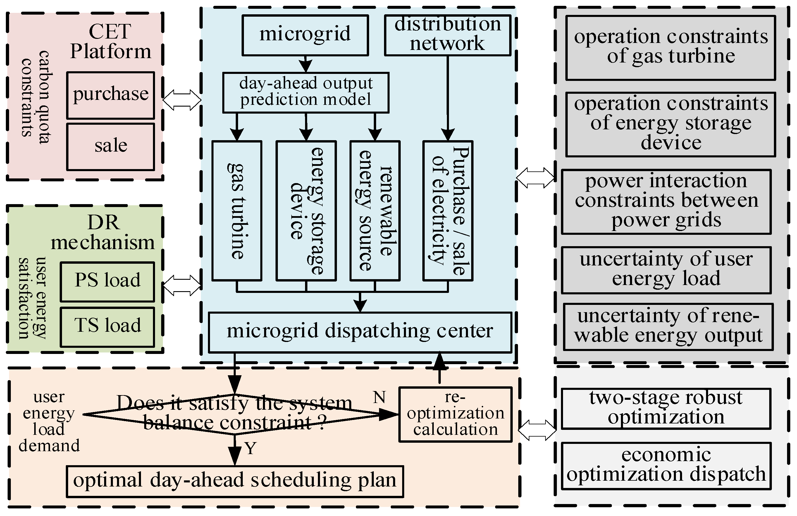
2. The Microgrid Operation Framework Considering Carbon-Trading Mechanism and Demand Response

2.1. System Operation Framework

This study explores the energy management system of a microgrid from both market and physical perspectives. On the physical side, it comprises of three types of producers: those who have renewable energy, gas turbine, and energy storage equipment installed. Moreover, there are microgrid transformers that combine the distributed loads of consumers and producers with power generation. Surplus electricity is given to the larger power grid, while those who need it can purchase from the primary power grid. On the market level, the microgrid dispatch center creates dispatch plans for electricity and equipment founded on the category of distributed energy installed by each consumer and the 24-h electricity price within the microgrid. The aim is to minimize electricity costs. The microgrid energy management system functions with the physical and market layers to achieve cost-effective operation and promote energy sharing between producers and consumers. In the carbon trading platform module, the microgrid dispatching center adjusts the output of the gas turbine according to the carbon quota and carbon price, and then decides whether to purchase the carbon quota. In the demand response mechanism module, the user adjusts the amount of electricity in the time of energy consumption based on changes in electricity prices to reduce costs. Aiming at the uncertainty of user energy load and distributed energy output, a two-stage optimization model incorporating robustness is utilized to achieve the objective of low-carbon economic dispatch. The microgrid optimization framework in this paper is shown in Figure 1.

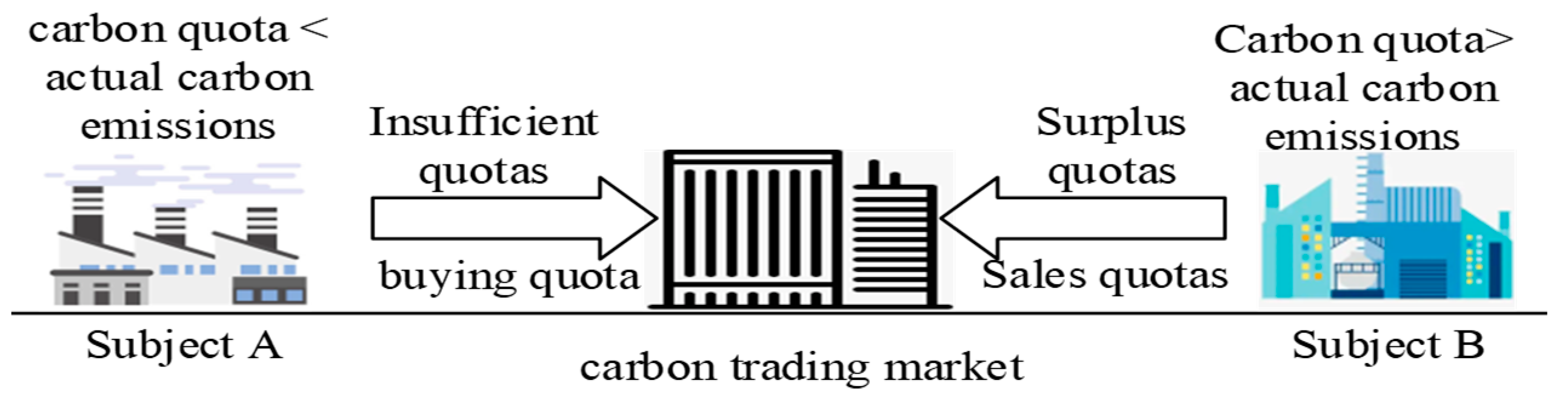
2.2. Carbon Emission Trading Mechanism

The Carbon Emission Trading (CET) mechanism is designed to regulate carbon dioxide emissions by establishing legal carbon emission rights and allowing these rights to be traded in the market. The aim of CET is to incentivize the assessed subject to reduce carbon emissions by imposing a cost. As shown in Figure 2, the assessment subject adjusts their production plan based on the carbon quota set by the regulatory authorities. The implementation of carbon trading will result in increased energy expenses and revenue for traditional power plants. As a result, this will impact the output ranking of distributed energy within the power system and enhance the efficiency of utilizing lower-emission power generation units.
The microgrid’s carbon emissions are based on the gas turbine’s output, and the carbon emissions of the system are represented in Equation (1).
E p = i = 1 N T t = 1 T b i P i , t
where E p is the system carbon emissions; N T is the number of gas turbine installed; T is the scheduling cycle; b i is the unit carbon emission coefficient ( t / ( k W h ) ) ; P i , t is the actual output produced by unit i in t period.
The baseline method is used to allocate the number of carbon quotas, and the allocation of carbon emission quotas is shown in Equation (2).
E q = i = 1 N T t = 1 T B i P i , t
where E q is the system carbon quota; B i is the reference value of power supply carbon emissions ( t / ( k W h ) ) .
Carbon trading mechanism in China is mainly divided into two forms: one is the traditional approach; the second is the ladder approach. The ladder approach involves the division of carbon dioxide emissions into various intervals. Different intervals have different carbon prices. The greater the amount of carbon dioxide emissions, the higher the cost per unit of emitted carbon dioxide from the system. The implementation of ladder carbon trading is better suited for the production of renewable energy and low-carbon units, and more conducive to reducing microgrid carbon emissions. For carbon emission control units, the ladder CET cost calculation model is shown in Equation (3).
C C E T = { C C O 2 ( Δ E ) Δ E l C C O 2 ( 1 + C O 2 ) ( Δ E l ) + C C O 2 l l < Δ E 2 l C C O 2 ( 1 + 2 C O 2 ) ( Δ E 2 l ) + C O 2 C C O 2 l + 2 C C O 2 l 2 l < Δ E 3 l C C O 2 ( 1 + 3 C O 2 ) ( Δ E 3 l ) + 3 C C O 2 C O 2 l + 3 C C O 2 l 3 l < Δ E
Δ E = E p E q
where C C E T represents the transaction cost for system participation in carbon emissions; C C O 2 is the price of the carbon market; l is the length of the interval for carbon emissions; C O 2 represents the rate of price growth; Δ E is the difference between the carbon emissions of the carbon emission control unit and the carbon quota. When it is negative, it indicates that the system’s carbon emissions are lower than the allocated amount. In this case, the excess quota can be sold at the initial carbon price.

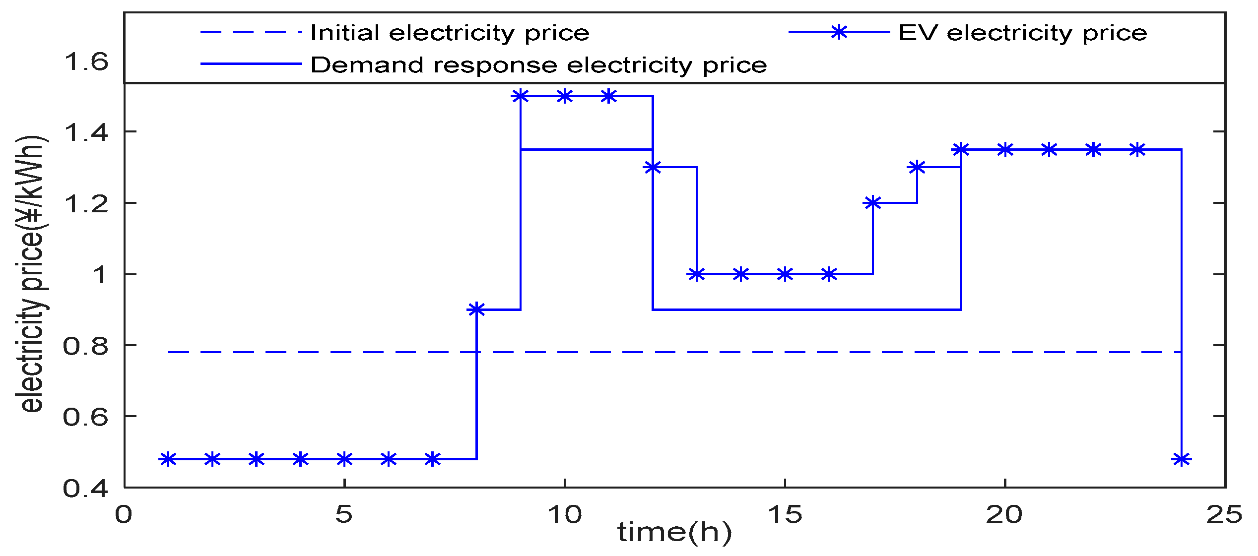
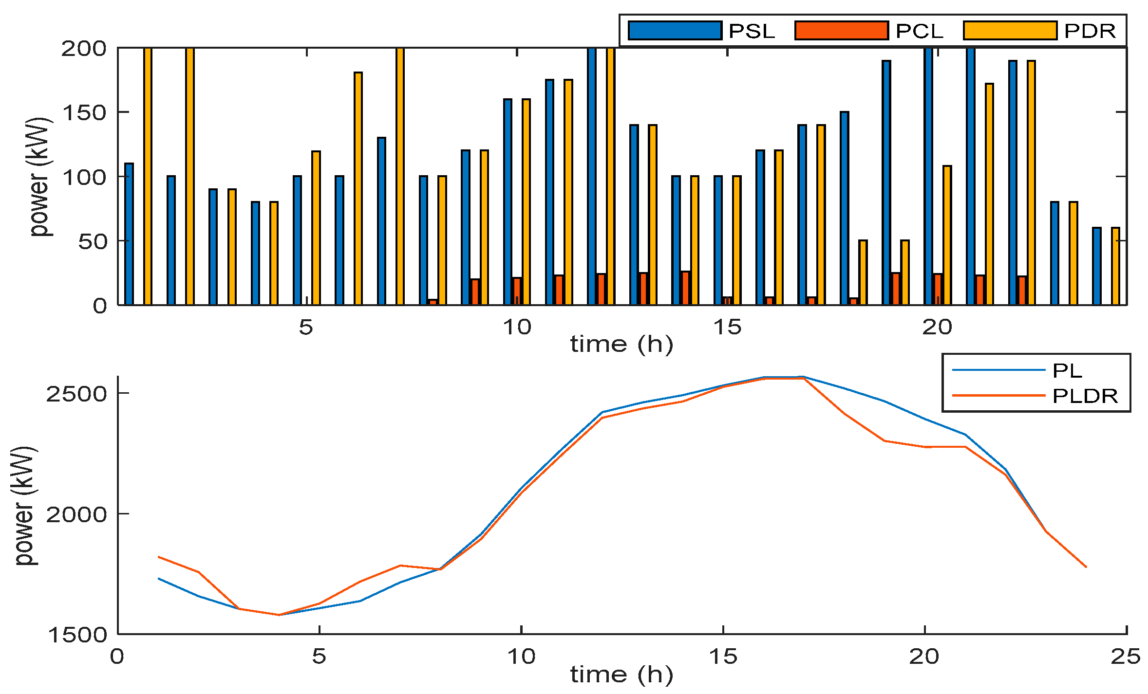
2.3. Demand Response Mechanism

The demand response (DR) mechanism refers to the user’s adjustment of energy consumption habits according to the electricity price or incentive mechanism to accomplish the goal of peak shaving and valley filling to enhance system stability. Based on varying load features, the DR types are price-sensitive and time-sensitive. For price-sensitive and time-sensitive types, their adjustable loads are defined as reducible loads and transferable loads, and they are modelled separately in this paper [35,36,37].
The elasticity matrix for prices and demand is utilized to depict the features of DR. The elasticity coefficient e i , j of the price at i period to the price at j period in the elasticity matrix E ( i , j ) is shown in Equation (5).
e i , j = Δ P L , t e / P L , t s t Δ ρ j / ρ j s t
where ρ j s t is the initial price at j period; P L , t s t is the initial load at t period; Δ ρ j is the change of electricity price at j period after participating in DR; and Δ P L , t e represents the load fluctuation participating in the DR.
The energy demand can be reduced by comparing the electricity price changes before and after the participation in the DR mechanism, thus deciding whether to decrease the energy load. The reducible loads P C L , t after participating in the demand response is shown in Equation (6).
P R L , t = P R L , t s t [ j = 1 24 E R L ( t , j ) ρ j ρ j s t ρ j s t ]
where P R L , t s t is the loads that can be reduced at t period; and E R L ( t , j ) is the matrix showing the elasticity of demand for price-reducible loads.
Transferable load refers to the difference in electricity prices that encourages consumers to adjust their energy consumption habits, helping shift peak loads to off-peak periods. The price–demand elasticity matrix is utilized to describe the DR dynamics, and the formula for transferable loads P T L , t is shown in Equation (7).
P T L , t = P T L , t s t [ j = 1 24 E T L ( t , j ) ρ j ρ j s t ρ j s t ]
where P S L , t s t  is the loads that can be transferable at t period; and E S L ( t , j ) is the matrix showing the elasticity of demand for transferable loads.
After the implementation of demand response, the total amount of transferable load in the scheduling cycle needs to remain unchanged, which is Equation (8). Due to the requirements of user comfort, the transfer load needs to meet Equation (9) in a period of time.
t = 1 T P D R , t = t = 1 T P T L , t
D D R min P D R , t D D R max
where P D R , t represents the true dispatching capability of the microgrid for meeting the DR load at t period and; D D R max and D D R min are the maximum/minimum electricity load of demand–response load in t period.
When consumers change their original electricity consumption habits, it will result in inconvenience, the degree of which will impact users’ willingness to engage in demand response. Therefore, the cost C D R of implementing the demand–response mechanism can be expressed as Equation (10), and the auxiliary variables P D R 1 , t and P D R 2 , t are introduced for convenient calculation as shown in Equations (11)–(13).
C D R = t = 1 T K D R ( | P D R , t P T L , t | + P R L , t )
P D R , t P T L , t + P D R 1 , t P D R 2 , t = 0
P D R 1 , t 0
P D R 2 , t 0
where K D R is the unit scheduling cost of reducible loads and transferable load.

2.4. Micro-Gas Turbine

The controllable power supply in the microgrid is mainly a gas turbine, and its cost of power generation is shown in Equation (14). The gas turbine must comply with power restrictions during operation, as shown in Equation (15).
C G = t = 1 T [ a P G , t + b ]
P G min P G , t P G max
where C G is the operating cost of the gas turbine; P G , t is the output power of gas turbine in t period; a , b are cost coefficients; and P G min and P G max are the maximum/minimum power in operation, respectively.

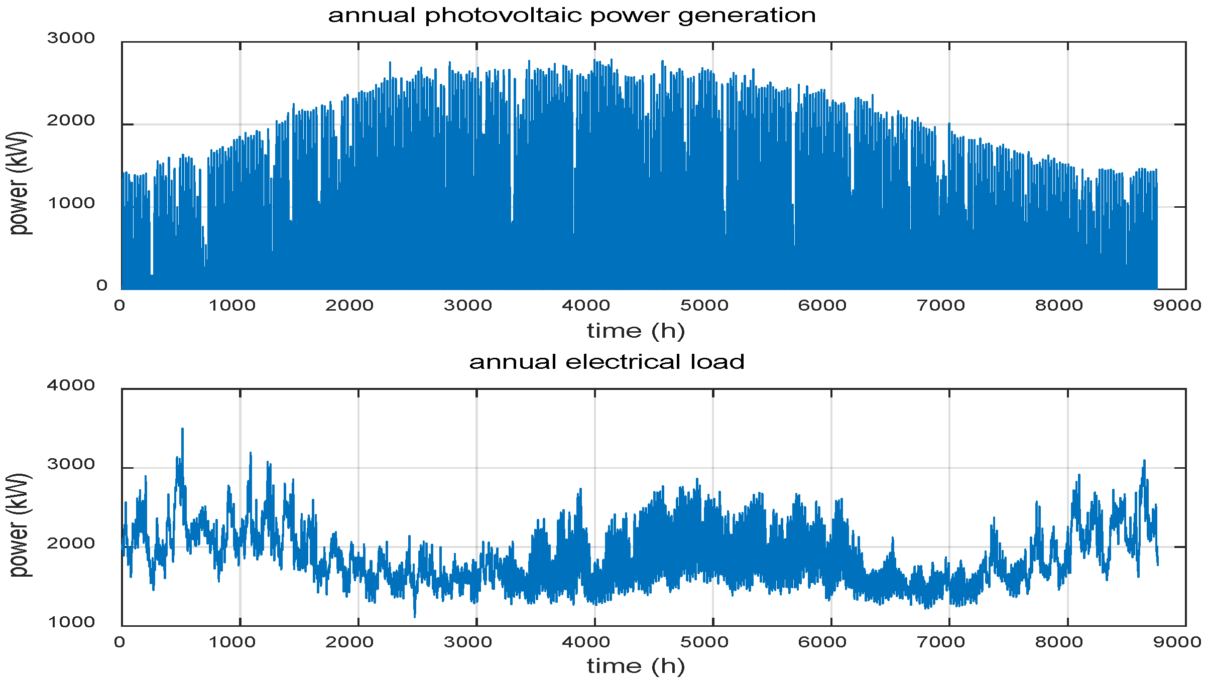
2.5. Renewable Energy Units

The maintenance cost of renewable energy units in the microgrid is shown in Equation (16), and the output of renewable units needs to meet the power constraints during operation, as shown in Equation (17).
C R = t = 1 T [ c P R , t + d ]
0 P R , t P R max
where C R  is the operating cost of renewable energy units; P R , t is the output of distributed energy at t period; c and d are the cost coefficient; and P R max is the maximum output of renewable energy prediction.

2.6. Energy Storage System

The fixed energy storage equipment has the characteristics of stabilizing power fluctuations and ensuring system stability during the operation of the microgrid. The operating cost C S includes the annualized value of the investment and the costs associated with operation and maintenance, as shown in Equation (18).
C S = t = 1 T K S [ P S , t d i s / η + P S , t c h η ] Δ t P S , t c h
where K S represents the cost of charging and discharging; P S , t c h and P S , t d i s are the charging/discharging power of the energy storage device during period t ; and η is the self-consumption rate of energy.
In the process of charging and discharging, the fixed energy storage equipment needs to meet the power constraints due to the capacity limitation of the grid-connected energy storage inverter device, as shown in Equations (19) and (20). Equation (21) shows that the energy storage device’s capacity should be equivalent at both the start and end of a full scheduling period. The battery’s state of charge during each period of the scheduling cycle must comply with the Equation (22) to effectively extend the longevity of the energy storage system.
0 P S , t d i s U S , t P S max
0 P S , t c h [ 1 U S , t ] P S max
η t = 1 T [ P S , t c h ] 1 η t = 1 T [ P S , t d i s ] = 0
E S min E S , t 1 + η t = 1 N T [ P S , t c h ] 1 η t = 1 N T [ P S , t d i s ] E S max
where P S max is the maximum charge/discharge power; U S , t is the charge/discharge state; E S max and E S min are the maximum/minimum residual capacity allowed by the battery state; and E S , t 1 is the state of charge of the battery at t 1 period.
Electric vehicles serve as mobile energy storage units and can be seamlessly integrated into the energy system, offering the same benefits as conventional energy storage devices. When there is excess power on the power supply side or the electricity price is low, electric vehicles can be charged. When the power is at its peak and the reliability of the power system is threatened, electric vehicles may discharge to the microgrid. In addition, to compensate the depreciation of electric vehicles, the electric vehicles discharge price is increased. Therefore, reasonable planning of electric vehicles not only provides flexibility in power system demand, but also offers benefits to electric vehicle owners. The operating cost of electric vehicles is shown in Equation (23) [38].
C E V = t = 1 T λ c ( t ) [ φ c λ c ( t ) P E V , t c h φ d λ d ( t ) P E V , t d i s ]
where P E V , t c h and P E V , t d i s are the quantity of electric vehicles charged/discharged t period; φ c and φ d  are the charging/discharging power of each electric vehicle; and λ c ( t ) and λ d ( t ) represent the prices for electric vehicle charging/discharging.
Considering the stability of the microgrid, the number of electric vehicles that can be used for charging or discharging within a unit scheduling time cannot exceed the maximum number of dispatches allowed by the microgrid, as shown in Equations (24) and (25). In addition, the total number of electric vehicles participating in microgrid scheduling in a scheduling cycle cannot exceed the actual number of available scheduling, as shown in Equations (26) and (27).
P E V , t c h P E V , t c h , max
P E V , t d i s P E V , t d i s , max
t = 1 T [ P E V , t c h ] P E V , max c h
t = 1 T [ P E V , t d i s ] P E V , max d i s
where P E V , t c h , max and P E V , t d i s , max are the maximum allowable number of electric vehicle charging/discharging at t period; and P E V , max c h and P E V , max d i s are the total number of electric vehicle charging/discharging in a scheduling cycle.

2.7. Grid Interactive System

The microgrid determines whether to procure or dispense electricity to the distribution network based on the internal load requirements and the power output of the power generation unit. The expenses C M associated with the collaboration between the distribution network and microgrid can be mathematically represented by the Equation (28). Due to the limitation of the capacity and number of transformers at the nodes, the interaction power between different networks needs to satisfy Equations (29) and (30).
C M = t = 1 T λ ( t ) [ P M , t b u y P M , t s e l l ]
0 P M , t b u y U M , t P M max
0 P M , t s e l l [ 1 U M , t ] P M max
where P M max is the maximum power of interaction with the distribution network; and U M , t is the state of purchase and sale; λ ( t ) is electricity price.
The microgrid needs to meet the balance between supply and demand of electric energy, and the energy balance constraint can be expressed as Equation (31).
P M , t b u y P M , t s e l l = P S , t c h + P D R , t + P L , t + φ c P E V , t c h P G , t P S , t d i s P R E , t φ d P E V , t d i s
where P M , t b u y and P M , t s e l l represent the electricity purchased and sold by the microgrid during the t period; P L , t and P R E , t are the user’s energy load power and the new energy output power in the microgrid.

3. Two-Stage Robust Optimization Model of Microgrid

3.1. Two-Stage Robust Optimization Model

In this paper, an optimal scheduling model is established with the aim of minimizing the comprehensive cost of microgrid operations during the scheduling period, as shown in Equation (32). The day-ahead scheduling plan includes the start–stop plan of gas turbines, energy storage equipment, photovoltaic units, unit output plan, carbon quota and electricity purchase and sale, and the load of demand–response adjustment.
{ min ( C C E T + C D R + C G + C R + C S + C E V + C M ) s . t .           E q u a t i o n s ( 11 ) ( 13 )           E q u a t i o n ( 15 )           E q u a t i o n ( 17 )           E q u a t i o n s ( 19 ) ( 22 )           E q u a t i o n s ( 24 ) ( 27 )           E q u a t i o n s ( 29 ) ( 31 )
where C C E T is Equation (3); C D R is Equation (10); C G is Equation (14); CR is Equation (16); C S is Equation (18); C E V is Equation (23); and C M is Equation (28).
The constraint condition D y d corresponds to Equations (9), (12), (13), (15), (17) and (24)–(27); K y = 0 corresponds to Equations (8), (11), (21) and (31); and F x + G y h corresponds to Equations (19), (20), (29) and (30).
{ min x , y   c T y s . t .     D y d     K y = 0     F x + G y h     I u y = u ^
{ x = [ U S , t , U M , t ] T y = [ P G , t , P R , t , P S , t c h , P S , t d i s , P D R , t P M , t b u y , P M , t s e l l , P E V , t c h , P E V , t d i s ] T u ^ = [ u ^ R E , t , u ^ L , t ] T t = ( 1 , 2 , , T )
where c represents the coefficient matrix of the objective function; D , K , F , G and I u represent the coefficients for the variables in their respective constraints; d and h are column vectors; u ^ R E , t and u ^ L , t , are the predicted values of renewable energy output and load.
Due to the uncertainty of distributed energy, deterministic optimization often cannot better adapt to the microgrid. Therefore, on the basis of Equation (33), this paper considers the fluctuation range of renewable energy output and user energy load, constructs the uncertainty set U as shown in Equation (35), and introduces the uncertainty adjustment parameters Γ R E and Γ L to regulate the conservatism. The increase of the value is to illustrate that the uncertainty set U changes towards a more adverse scenario. The classical polyhedron uncertainty set characterizes the uncertainty of photovoltaic output and load power consumption by scaling the upper and lower bounds of the interval, which often results in too conservative scheduling results. In this paper, the probability characteristic information of distributed energy to reduce the conservatism of decision results. In view of the uncertainty of distributed energy that can be represented as a normal distribution prediction error, this paper optimizes the interval [39,40].
U = { u R E , t = u ^ R E , t + B R E , t + Δ u R E , t max B R E , t Δ u R E , t max 0 B R E , t + + B R E , t 1 Δ u R E , t max = z α / 2 σ R E / n t = 1 N T ( B R E , t + + B R E , t ) Γ R E u L , t = u ^ L , t + B L , t + Δ u L , t max B L , t Δ u L , t max Δ u L , t max = z α / 2 σ L / n 0 B L , t + + B L , t 1 t = 1 N T ( B L , t + + B L , t ) Γ L 0 Γ R E , Γ L T u = [ u R E , t , u L , t ] T
where u R E , t and u L , t are uncertain variables of renewable energy output and user energy load; Δ u R E , t max and Δ u L , t max are the maximum permissible deviation of renewable energy output and load; B R E , t + , B R E , t , B L , t + and B L , t are 0–1 variables; σ R E and σ L are the standard deviation of the predicted value; n is the sample size; z α / 2 is the two-sided quantile of the standard normal distribution; and α is the significance level.
Renewable energy output often has a specific spatial–temporal correlation. By considering the correlation between space and time, it is possible to eliminate scenarios that have a low probability density, thus reducing excess caution. Therefore, based on the Pearson correlation coefficient, this paper constrains the auxiliary variables of the uncertainty adjustment parameters, as shown in Equation (36).
{ ζ R E , t u + B R E , t + B R E , t + 1 + ζ R E , t d + ζ R E , t u B R E , t B R E , t + 1 ζ R E , t d t = 1 N T ( ζ R E , t u + + ζ R E , t d + + ζ R E , t u + ζ R E , t d ) Γ t 0 ζ R E , t u + , ζ R E , t d + , ζ R E , t u , ζ R E , t d 1 ζ s [ B R E , t + Δ u R E , t max B R E , t Δ u R E , t max u R E , t                             B R E , t + Δ u R E , t max B R E , t Δ u R E , t max u R E , t ] ζ s
where ζ R E , t u + , ζ R E , t d + , ζ R E , t u and ζ R E , t d are the binary variables of renewable energy units in the time series; Γ t is the time correlation coefficient of uncertain adjustment parameters; and ζ s is the spatial correlation coefficient of uncertain adjustment parameters.
After defining the uncertainty set U, a two-stage robust optimization model is formulated as illustrated in Equation (37). The expressions of x and y  are shown in Equation (34). The outer layer min x {   } indicates the overall operating cost is the lowest, which is the first-stage problem. The inner layer max u U min y Ω ( x , u ) c T y is the second stage problem. Ω ( x , u ) is feasible region of y when ( x , u ) is known, as shown in Equation (38).
{ min x { b T x + max u U min y Ω ( x , u ) c T y } s . t .     D y d   γ     K y = 0   λ     F x + G y h   ν     I u y = u ^   π
Ω ( x , u ) = { D y d   K y = 0   F x + G y h   I u y = u ^
where γ , λ , ν and π are the dual variables in the dual model of Equation (37).

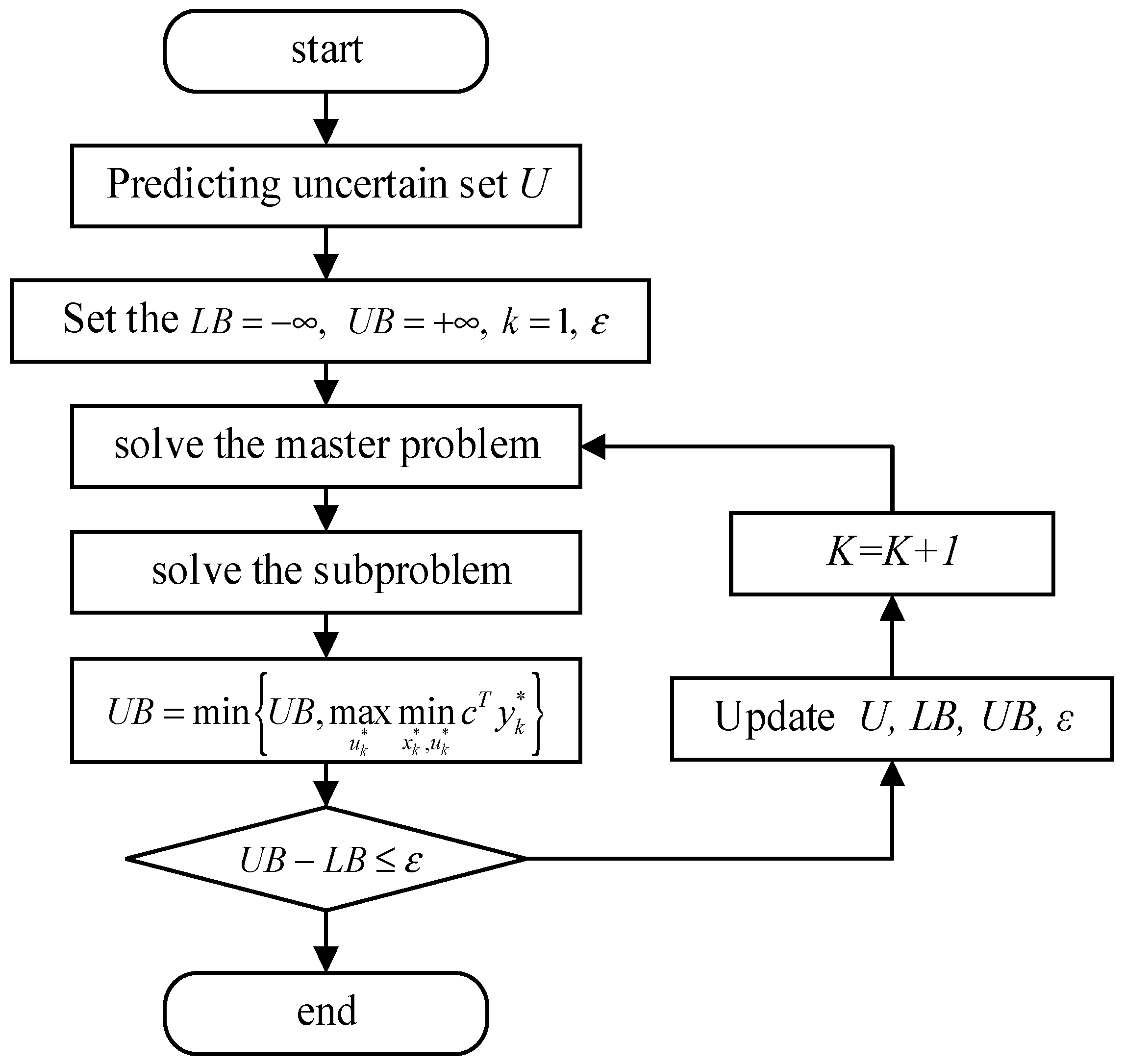
3.2. Column Constraint Generation Algorithm

This paper applies the column-and-constraint generation (C&CG) algorithm to divide the original problem into a primary problem and a subsidiary problem. The C&CG algorithm effectively enhances the speed of computation by continuously incorporating the optimal subproblem value while solving the main problem. The resulting two-stage robust optimization model is broken down into the main problem, which is presented as Equation (39).
{ min x , y   b T x + c T y s . t .     c T y c T y k 1     D y d     K y = 0     F x + G y h     I u y = u k 1 *
where k is the current number of iterations; β is the auxiliary variable; y k 1 is the optimal solution after the ( k 1 )th iteration; and u k 1 * is the value of the u after the ( k 1 )th iteration.
The decomposed subproblem max u U min y Ω ( x , u ) c T y is a linear problem under a given ( x , u ) . According to the dual theory, the inner min problem is converted into max problem, as shown in Equation (40).
{ max u U , γ , λ , ν , π d T γ + ( h F x T ) T ν + u T π s . t .     D T γ + K T λ + G T ν + I u T π c     γ 0 , ν 0 , π 0
The uncertainty set U is substituted into the Equation (32), and the variable product part is changed to obtain the modified subproblem Equation (41).
{ max B , B , γ , λ , ν , π d T γ + ( h F x T ) T ν + u ^ T π + Δ u T B s . t .     D T γ + K T λ + G T ν + π I u T c     γ 0 , ν 0 , π 0     0 B M B     π M ( 1 B ) B π     0 B R E , t + + B R E , t 1     0 B L , t + + B L , t 1     t = 1 N T ( B R E , t + + B R E , t ) Γ R E     t = 1 N T ( B L , t + + B L , t ) Γ L
where Δ u = [ Δ u P V ( t ) , Δ u L ( t ) ] T ; B = [ B R E , t + , B R E , t , B L , t + , B L , t ] T ; B = [ B R E , t + , B R E , t , B L , t + , B L , t ] T ; and M is a positive number of any size (not infinity).
Following the aforementioned conversion, the two-stage robust model is ultimately converted into a mixed-integer programming problem, including the main problem Equation (39) and the subproblem Equation (41). The algorithm flow is shown in Figure 3.
(1)
Prediction of renewable energy output and user energy load uncertainty set U.
(2)
Define the lower bound L B = , the upper bound U B = + , number of iterations k = 1 , convergence threshold ε .
(3)
Take the predicted value of the uncertainty set as the initial scenario u ^ and bring it into the main problem Equation (39).
(4)
The optimal solution ( x k * , y k * ) for the initial deterministic model has been attained, and the lower bound L B = c T y k * of the operating cost is updated.
(5)
Substituting x k * into the subproblem Equation (41), the objective function value A and the corresponding uncertain variable A of the subproblem are solved, and the upper bound is updated.
(6)
Judging U B L B ε , if it is established, the iteration is stopped and the optimal solution ( x k * , y k * ) is returned; otherwise, add the constraint c T y c T y k * to the main problem and run step 3 until the algorithm converges to the threshold ε .

4. Results and Discussion
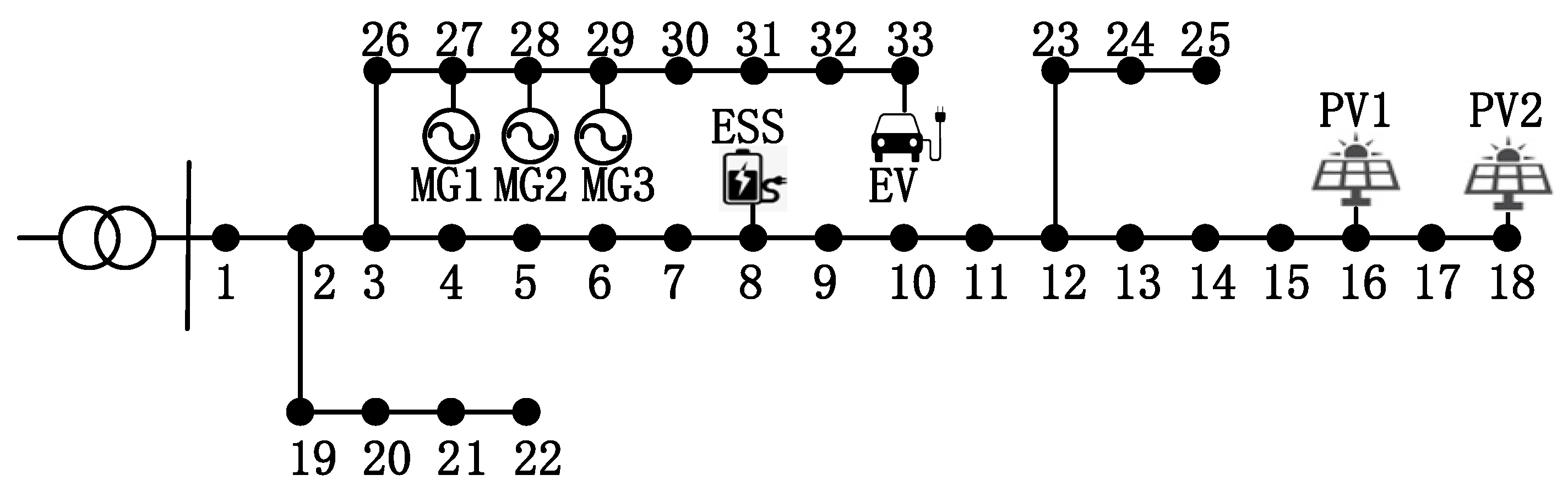
4.1. Parameters

To validate the practicality and efficiency of the proposed two-stage robust optimization strategy based on carbon trading and demand response, this section constructs a microgrid simulation model, including micro-gas turbines, photovoltaic units, energy storage equipment and electric vehicles, which is modified on the basis of IEEE-33 node. The system topology is shown in Figure 4. Using a scheduling cycle of 24 h, the unit scheduling interval is set at 1 h, and the unit parameters are outlined in Table 1. The battery parameters of electric vehicles refer to energy storage equipment. There are 15,000 electric vehicles within the microgrid coverage area. The electric vehicles’ average power of charging and discharging electric vehicles is 30 kW. Users begin to charge electric vehicles after returning home from work. The transaction price is shown in Figure 5. In the carbon-trading module, the CET price is set to 50 CNY/t, the length of the interval for CET is 500 t, and the rate of CET price increase is 25%. In the demand–response module, fixed, transferable, and reducible loads account for 70%, 20%, and 10% of the total load, respectively. The uncertainty of photovoltaic prediction and user energy load prediction are six and 12, respectively, and the remaining time prediction value is accurate.
The uncertainties considered in this paper include load forecasting and photovoltaic power generation forecasting errors. The forecasting errors of photovoltaic load power are subject to normal distribution. The photovoltaic units and loads in a region within one year are analyzed, as shown in Figure 5. The data were subjected to cluster analysis, with the results presented in Figure 6. Based on the probability of each typical scene, typical data five are selected as the experimental data. It can be seen that the large probability of photovoltaic unit output time appears at 6–18 o’clock, while the rest of the time there is no output. The output is the largest at 11–14 o’clock. The load data have a peak at 11–13 o’clock and a valley at 2–10 o’clock.

4.2. Analysis of Scheduling Results

In this paper, the maximum allowable fluctuation deviation of power load and photovoltaic output in a microgrid is determined based on the load deviation depicted in Figure 7, where different curves represent different scenarios of power. Figure 8 shows the predicted/actual load power curve and the maximum PV output curve. The scheduling optimization results are shown in Figure 9.
When the microgrid sells electricity to the distribution network, the value is negative, and the value is positive when purchasing. Due to varying electricity prices during peak and off-peak hours, the microgrid purchases power from the grid between 1–8 o’clock and 14–24 o’clock, while selling excess energy back to the grid between 9–13 o’clock. Due to the photovoltaic output, the microgrid purchases less power from the distribution network at 8 o’clock and 14–17 o’clock, and the microgrid sales reach the maximum at 10–13 o’clock when the photovoltaic output is the largest.
When both micro-gas turbines and photovoltaic units perform power, the value is positive. At 1–7 o’clock and 24 o’clock, the cost of purchasing electricity for a microgrid is lower than the cost of generating electricity using a micro-gas turbine. At this time, the output power of the micro-gas turbine in the microgrid is lower. The electricity purchase cost is higher at 8–23 o’clock, and the micro-gas turbine output reaches the maximum output to reduce the operation cost of the microgrid.
When the fixed energy storage equipment and the mobile energy storage equipment with electric vehicles as the main body are charged, the value is negative, and the value is positive when discharged. According to the time-of-use electricity price mechanism shown in Figure 5, as a result of varying electricity rates during peak, flat, and valley periods, utilizing energy storage to transport electricity from off-peak to on-peak periods can significantly minimize operating costs within microgrids. In the trough of electricity prices, electric vehicles are charged at 1–2 o’clock. When the photovoltaic output is stable, electric vehicle charging and fixed energy storage equipment charging take place at 7 o’clock. At the peak of electricity price, there is electric vehicle discharge at 9–11 o’clock, and there is fixed energy storage equipment discharge at 19 o’clock. It is evident that the output of the stationary energy storage apparatus is less than the installed stationary energy storage capacity in the microgrid. This is because the expense of the energy storage unit is greater compared to the cost of scheduling energy storage based on the time-of-use electricity pricing mechanism. It has been estimated that the efficiency of stationary energy storage systems can be greatly enhanced by a 10% reduction in the charging and discharging unit costs. Therefore, if there is no incentive policy for fixed energy storage equipment, it is not necessary to install fixed energy storage only considering the benefit of load peak shaving and valley filling. Mobile energy storage represented by electric vehicles can help with peak shaving and valley filling.

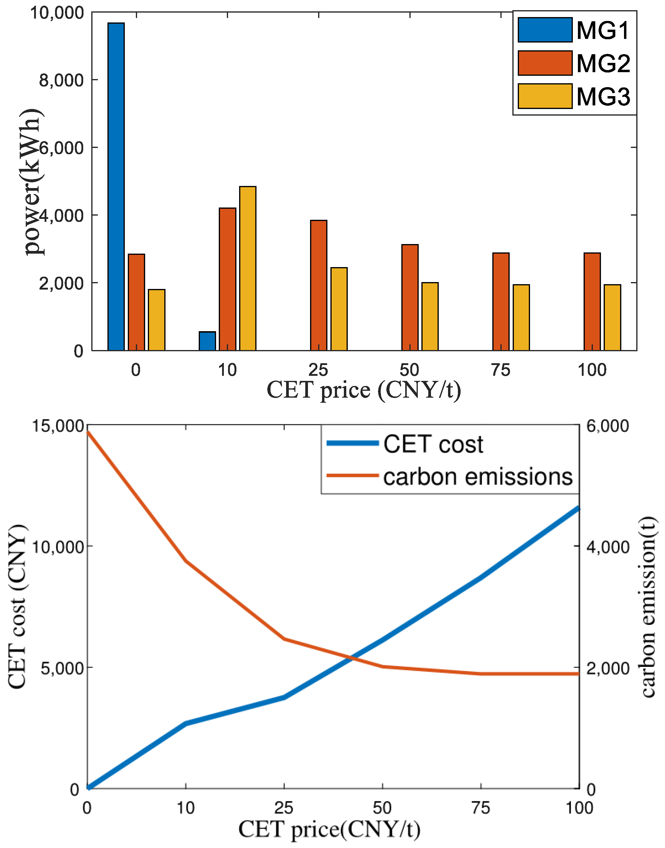
4.3. Analysis of Carbon Trading Mechanism

Figure 10 illustrates the correlation between the CET price and the operational expenses of the microgrid. As the CET price rises from 0 to 100 CNY/t, the associated costs escalate dramatically while the carbon footprint of the system reduces in proportion. Due to the higher CET price, the microgrid dispatch center limits the output of units with higher carbon emission levels, which in turn increases the output of low-carbon and renewable energy units. When the CET price is 0 CNY/t, there is no carbon market. Currently, the micro-gas turbine has a maximum output of 14,319 kW, and the carbon emission is 5885.06 t. In the process of CET price increasing from 75 CNY/t to 100 CNY/t, the output of the micro-gas turbine is gradually reduced. The output of the unit MG1 with the highest carbon emission coefficient decreases the fastest, and the output of the low-carbon units MG2 and MG3 increases slightly. With the increase in the CET price, carbon emissions decreased by 36.2%, 58.1%, 65.9%, 67.9% and 67.9%. At the same time, the cost of CET gradually increased by 2677.68 CNY, 1076.58 CNY, 2369.75 CNY, 2572.25 CNY and 2898.75 CNY. When the CET price is 100 CNY/t, due to the need to meet the system power balance, although the CET price increases at this time, the carbon emissions will not decrease. Therefore, carbon emissions can be effectively reduced within a certain range through the use of CET pricing. Setting the CET price too high, however, would only lead to increased operating costs for the microgrid without any corresponding decrease in carbon emissions.

4.4. Analysis of Demand Response Mechanism

As illustrated in Figure 11, guided by electricity prices, the demand–response mechanism shifts the movable load from high-price to low-price periods, thereby reducing transferable load. Peak-time loads (8–12 h and 17–21 h) decrease, while trough-time loads (1–7 h, 13–16 h, and 22–23 h) increase correspondingly, reducing the microgrid’s need to purchase power during peak-price periods. Therefore, the DR mechanism empowers transmittable loads to react to signals of electricity prices and efficiently enhance the efficiency of the microgrid. In addition, by increasing the compensation cost K D R for user participation in DR by 10%, the electricity consumption for user participation in DR will increase, and the effect of peak shaving and valley filling will be more significant, but it will lead to an increase in the operating cost of the microgrid. After reducing the compensation cost K D R for user participation in DR by 10%, the electricity consumption for user participation in DR is reduced, which limits its potential for peak shaving and valley filling. Therefore, it is necessary to reasonably set the compensation cost of demand response, taking into account the economy and stability.

4.5. Uncertainty Analysis

To assess the efficacy of the optimization approach outlined in enhancing system stability, five distinct configurations of uncertainty adjustment parameters are chosen for comparative simulation analysis. The relevant parameter setups and operational expenses are outlined in Table 2. A higher value of the uncertainty adjustment parameter corresponds to a longer duration, over which the load power attains the maximum value of the prediction interval and the photovoltaic output reaches the minimum value of the prediction interval. With the increase in the uncertainty adjustment parameters, the uncertainty faced by the microgrid in formulating the day-ahead scheduling strategy increases, the conservatism of the obtained scheme increases, and the corresponding operating cost increases. The rise in operational costs is primarily attributable to increased electricity procurement expenses and reduced electricity sales from the microgrid to the distribution network. When the uncertainty adjustment parameters are all zero, the optimization model is a deterministic optimization model, and the scheduling result is shown in Figure 12. Comparing the two-stage optimal scheduling results in Figure 9, it is evident that the microgrid is currently selling electricity to the distribution network at a higher rate than when the uncertain adjustment parameters are six and 12. As shown in Table 2, the operating cost of the scheduling scheme derived from the deterministic optimization approach is lower than that of the approach proposed in this paper. However, this does not necessarily imply that the deterministic approach is superior to the robust method. Comparing the optimal scheduling results of the two-stage process shown in Figure 9, it is apparent that the microgrid’s sale of electricity to the distribution network is currently higher than when the uncertain adjustment parameters are six and 12. The deterministic optimization method’s operation cost in Table 2 is lower than that of the robust optimization method, but it does not signify that the deterministic approach is superior to the robust one. This is due to the mismatch between the distributed power output and the actual output caused by the forecasting error, which leads to the need for the microgrid to purchase electricity in the real-time power market for compensation. Moreover, the current cost of purchasing electricity in real-time exceeds that of the day-ahead market, resulting in a higher overall transaction expense for the microgrid.

5. Conclusions

This paper explores carbon-trading mechanisms, demand–response mechanisms, and the uncertainty of distributed energy. A two-stage robust optimization model is designed for microgrids. By simulating dispatching results in different scenarios, the following conclusions can be drawn:
(1)
Considering the uncertainty of distributed generation, this paper flexibly adjusts the conservatism of microgrid optimization work through a two-stage robust optimization model. The approach results in a scheduling strategy that ensures the lowest system operation cost under unfavorable conditions, facilitating the rational allocation and utilization of resources and enhancing the economic and operational stability of the microgrid.
(2)
Based on the carbon-trading mechanism, this paper effectively coordinates the economy and low carbon of microgrid operations. By comparing the impact of CET price on the optimal operation results, it concludes that the system’s total operating expenses increase as the CET rate rises, while carbon emissions gradually decrease in response to changes in the carbon exchange price. Additionally, implementing a suitable carbon exchange pricing system can align low-carbon initiatives with economic goals.
(3)
This paper introduces an energy storage system and demand–response mechanism that can greatly reduce operating costs. When operating under a time-of-use electricity pricing mechanism, the microgrid scheduling plan of the microgrid relies on the peak–valley electricity price differential and the expenses associated with charging and discharging the energy storage unit. By implementing an energy storage system, both the cost of wasted electricity and the cost of purchased electricity can be reduced. By storing surplus photovoltaic power during periods of low demand and releasing it during peak periods, more advantages can be gained.
The scheduling strategy proposed in this paper adopts a conservative approach. With a focus on economic and low carbon principles, the stability of the power system can be enhanced when dealing with large-scale integration of intermittent and random renewable energy sources, thus avoiding the occurrence of wind and light abandonment. This model is beneficial for promoting sustainable development within the power system by enabling the large-scale integration of renewable energy sources. Regarding the operating characteristics of various devices in microgrids, nonlinear modelling poses a significant challenge for solving optimization models, and therefore, linear models are commonly used in papers to describe them. However, to comprehensively reflect the true operating characteristics of microgrids, further in-depth research is needed to explore nonlinear modeling and solving methods suitable for optimization and operation issues in microgrids.

Author Contributions

Conceptualization, Y.Z.; methodology, W.H.; software, T.L.; validation, T.L.; data curation, T.L.; writing—original draft, T.L. writing—review and editing, Y.Z.; supervision, W.H.; project administration, W.H. All authors have read and agreed to the published version of the manuscript.

Funding

This research was funded by the Project of the National Social Science Fund of China, grant number 19BGL003.

Institutional Review Board Statement

Not applicable.

Informed Consent Statement

Not applicable.

Data Availability Statement

Not applicable.

Conflicts of Interest

The authors declare no conflict of interest.

References

  1. Dong, L.; Miao, G.; Wen, W. China’s carbon neutrality policy: Objectives, impacts and paths. East Asian Policy 2021, 13, 5–18. [Google Scholar] [CrossRef]
  2. Hu, Y.; Chi, Y.; Zhou, W.; Wang, Z.; Yuan, Y.; Li, R. Research on energy structure optimization and carbon emission reduction path in Beijing under the Dual Carbon Target. Energies 2022, 15, 5954. [Google Scholar] [CrossRef]
  3. Ma, M.; Cai, W.; Cai, W. Carbon abatement in China’s commercial building sector: A bottom-up measurement model based on Kaya-LMDI methods. Energy 2018, 165, 350–368. [Google Scholar] [CrossRef]
  4. Zhang, X.P.; Cheng, X.M. Energy consumption, carbon emissions, and economic growth in China. Ecol. Econ. 2019, 68, 2706–2712. [Google Scholar] [CrossRef]
  5. Wang, Y.; Qiu, J.; Tao, Y.; Zhao, J. Carbon-oriented operational planning in coupled electricity and emission trading markets. IEEE Trans. Power Syst. 2020, 35, 3154–3157. [Google Scholar] [CrossRef]
  6. Li, J.; Mao, T.; Huang, G.; Zhao, W.; Wang, T. Research on Day-Ahead Optimal Scheduling Considering Carbon Emission Allowance and Carbon Trading. Sustainability 2023, 15, 6108. [Google Scholar] [CrossRef]
  7. Cui, Y.; Zeng, P.; Zhong, W.; Cui, W.; Zhao, Y. Low-carbon economie dispatch of electricity-gas-heat integrated energy system based on ladder-type carbon trading. Electr. Power Autom. Equip. 2021, 41, 10–17. [Google Scholar]
  8. Akulker, H.; Aydin, E. Optimal design and operation of a multi-energy microgrid using mixed-integer nonlinear programming: Impact of carbon cap and trade system and taxing on equipment selections. Appl. Energy 2023, 330, 120313. [Google Scholar] [CrossRef]
  9. Yan, L.; Zhao, Y.; Xue, T.; Ma, N.; Li, Z.; Yan, Z. Two-Layer Optimal Operation of AC–DC Hybrid Microgrid Considering Carbon Emissions Trading in Multiple Scenarios. Sustainability 2022, 14, 10524. [Google Scholar] [CrossRef]
  10. Zhou, Q.; Zhang, J.; Gao, P.; Zhang, R.; Liu, L.; Wang, S.; Cheng, L.; Wang, W.; Yang, S. Two-Stage Robust Optimization for Prosumers Considering Uncertainties from Sustainable Energy of Wind Power Generation and Load Demand Based on Nested C&CG Algorithm. Sustainability 2023, 15, 9769. [Google Scholar]
  11. Saeed, M.H.; Wang, F.Z.; Kalwar, B.A.; Iqbal, S. A Review on Microgrids’ Challenges & Perspectives. IEEE Access 2021, 9, 166502–166517. [Google Scholar]
  12. Yaqoob, M.; Lashab, A.; Vasquez, J.C.; Guerrero, J.M.; Orchard, M.E.; Bintoudi, A.D. A Comprehensive Review on Small Satellite Microgrids. IEEE Trans. Power Electron. 2022, 37, 12741–12762. [Google Scholar] [CrossRef]
  13. Khan, A.A.; Naeem, M.; Iqbal, M.; Qaisar, S.; Anpalagan, A. A compendium of optimization objectives, constraints, tools and algorithms for energy management in microgrids. Renew. Sustain. Energy Rev. 2016, 58, 1664–1683. [Google Scholar] [CrossRef]
  14. Bahramara, S.; Sheikhahmadi, P.; Golpîra, H. Co-optimization of energy and reserve in standalone micro-grid considering uncertainties. Energy 2019, 176, 792–804. [Google Scholar] [CrossRef]
  15. Hadayeghparast, S.; Farsangi, A.S.; Shayanfar, H. Day-ahead stochastic multi-objective economic/emission operational scheduling of a large scale virtual power plant. Energy 2019, 172, 630–646. [Google Scholar] [CrossRef]
  16. Kong, X.; Liu, D.; Wang, C.; Sun, F.; Li, S. Optimal operation strategy for interconnected microgrids in market environment considering uncertainty. Appl. Energy 2020, 275, 115336. [Google Scholar] [CrossRef]
  17. Cao, B.; Dong, W.; Lv, Z.; Gu, Y.; Singh, S.; Kumar, P. Hybrid Microgrid Many-Objective Sizing Optimization With Fuzzy Decision. IEEE Trans. Fuzzy Syst. 2020, 28, 2702–2710. [Google Scholar] [CrossRef]
  18. Jiang, J.; Zhang, L.; Wen, X.; Valipour, E.; Nojavan, S. Risk-based performance of power-to-gas storage technology integrated with energy hub system regarding downside risk constrained approach. Int. J. Hydrog. Energy 2022, 47, 39429–39442. [Google Scholar] [CrossRef]
  19. Zheng, S.; Shahzad, M.; Asif, H.M.; Gao, J.; Muqeet, H.A. Advanced optimizer for maximum power point tracking of photovoltaic systems in smart grid: A roadmap towards clean energy tech-nologies. Renew. Energy 2023, 206, 1326–1335. [Google Scholar] [CrossRef]
  20. Deng, W.; Zhang, Y.; Tang, Y.; Li, Q.; Yi, Y. A neural network-based adaptive pow-er-sharing strategy for hybrid frame inverters in a microgrid. Front. Energy Res. 2023, 10, 1082948. [Google Scholar] [CrossRef]
  21. Dong, J.; Yang, P.; Nie, S. Day-Ahead Scheduling Model of the Distributed Small Hydro-Wind-Energy Storage Power System Based on Two-Stage Stochastic Robust Optimization. Sustainability 2019, 11, 2829. [Google Scholar] [CrossRef]
  22. Naji Alhasnawi, B.; Jasim, B.H.; Esteban, M.D. A New Robust Energy Management and Control Strategy for a Hybrid Microgrid System Based on Green Energy. Sustainability 2020, 12, 5724. [Google Scholar] [CrossRef]
  23. Lotfi Akbarabadi, M.; Sirjani, R. Achieving Sustainability and Cost-Effectiveness in Power Generation: Multi-Objective Dispatch of Solar, Wind, and Hydro Units. Sustainability 2023, 15, 2407. [Google Scholar] [CrossRef]
  24. Wang, X.; Zhao, H.; Xie, G.; Lin, K.; Hong, J. Research on Industrial and Commercial User-Side Energy Storage Planning Considering Uncertainty and Multi-Market Joint Operation. Sustainability 2023, 15, 1828. [Google Scholar] [CrossRef]
  25. Li, Q.; Li, Q.; Wang, C. Unit Combination Scheduling Method Considering System Frequency Dynamic Constraints under High Wind Power Share. Sustainability 2023, 15, 11840. [Google Scholar] [CrossRef]
  26. Chen, T.; Gan, L.; Iqbal, S.; Jasiński, M.; El-Meligy, M.A.; Sharaf, M.; Ali, S.G. A Novel Evolving Framework for Energy Management in Combined Heat and Electricity Systems with Demand Response Programs. Sustainability 2023, 15, 10481. [Google Scholar] [CrossRef]
  27. de Souza Dutra, M.D.; da Conceição Júnior, G.; de Paula Ferreira, W.; Chaves, M.R. A customized transition towards smart homes: A fast framework for economic analyses. Appl. Energy 2020, 262, 114549. [Google Scholar] [CrossRef]
  28. Zhang, Y.; Ai, X.; Wen, J.; Fang, J.; He, H. Data-adaptive robust optimization method for the economic dispatch of active distribution networks. IEEE Trans. Smart Grid 2018, 10, 3791–3800. [Google Scholar] [CrossRef]
  29. Wu, J.; Tan, Z.; Wang, K.; Liang, Y.; Zhou, J. Research on Multi-Objective Optimization Model for Hybrid Energy System Considering Combination of Wind Power and Energy Storage. Sustainability 2021, 13, 3098. [Google Scholar] [CrossRef]
  30. Dashtdar, M.; Flah, A.; Hosseinimoghadam, S.M.S.; Kotb, H.; Jasińska, E.; Gono, R.; Leonowicz, Z.; Jasiński, M. Optimal Operation of Microgrids with Demand-Side Management Based on a Combination of Genetic Algorithm and Artificial Bee Colony. Sustainability 2022, 14, 6759. [Google Scholar] [CrossRef]
  31. AlDavood, M.S.; Mehbodniya, A.; Webber, J.L.; Ensaf, M.; Azimian, M. Robust Optimization-Based Optimal Operation of Islanded Microgrid Considering Demand Response. Sustainability 2022, 14, 14194. [Google Scholar] [CrossRef]
  32. Yu, J.; Liu, J.; Wen, Y.; Yu, X. Economic Optimal Coordinated Dispatch of Power for Community Users Considering Shared Energy Storage and Demand Response under Blockchain. Sustainability 2023, 15, 6620. [Google Scholar] [CrossRef]
  33. Qiu, H.; Long, H.; Gu, W.; Pan, G. Recourse-Cost Constrained Robust Optimization for Microgrid Dispatch With Correlated Uncertainties. IEEE Trans. Ind. Electron. 2021, 68, 2266–2278. [Google Scholar] [CrossRef]
  34. Zhong, J.; Cao, Y.; Li, Y.; Tan, Y.; Peng, Y.; Cao, L.; Zeng, Z. Distributed modeling considering uncertainties for robust operation of integrated energy system. Energy 2021, 224, 120179. [Google Scholar] [CrossRef]
  35. He, L.; Lu, Z.; Geng, L.; Zhang, J.; Li, X.; Guo, X. Environmental economic dispatch of integrated regional energy system considering integrated demand response. Int. J. Electr. Power Energy Syst. 2020, 116, 105525. [Google Scholar] [CrossRef]
  36. Fan, W.; Tan, Z.; Li, F.; Zhang, A.; Ju, L.; Wang, Y.; De, G. A two-stage optimal scheduling model of integrated energy system based on CVaR theory implementing integrated demand response. Energy 2023, 263, 125783. [Google Scholar] [CrossRef]
  37. Sun, W.; Gong, Y.; Luo, J. Energy Storage Configuration of Distribution Networks Considering Uncertainties of Generalized Demand-Side Resources and Renewable Energies. Sustainability 2023, 15, 1097. [Google Scholar] [CrossRef]
  38. He, L.; Yang, J.; Yan, J.; Tang, Y.; He, H. A bi-layer optimization based temporal and spatial scheduling for large-scale electric vehicles. Appl. Energy 2016, 168, 179–192. [Google Scholar] [CrossRef]
  39. Xu, H.; Meng, Z.; Wang, Y. Economic dispatching of microgrid considering renewable energy uncertainty and demand side response. Energy Rep. 2020, 6, 196–204. [Google Scholar] [CrossRef]
  40. Yin, M.; Li, K.; Yu, J. A data-driven approach for microgrid distributed generation planning under uncertainties. Appl. Energy 2022, 309, 118429. [Google Scholar] [CrossRef]
Figure 1. Day-ahead optimal scheduling framework of microgrid.
Sustainability 15 14592 g001
Figure 2. Schematic diagram of carbon trading principle.
Sustainability 15 14592 g002
Figure 3. Comparison of unit output in different scenarios.
Sustainability 15 14592 g003
Figure 4. System topology of microgrid.
Sustainability 15 14592 g004
Figure 5. Electricity price plan.
Sustainability 15 14592 g005
Figure 6. Statistics of photovoltaic units and loads during the year.
Sustainability 15 14592 g006
Figure 7. Cluster analysis result.
Sustainability 15 14592 g007
Figure 8. Predicted/actual load curve.
Sustainability 15 14592 g008
Figure 9. Comparison of unit output.
Sustainability 15 14592 g009
Figure 10. CET mechanism sensitivity.
Sustainability 15 14592 g010
Figure 11. Consequence of demand response.
Sustainability 15 14592 g011
Figure 12. Comparison of unit output.
Sustainability 15 14592 g012
Table 1. Operation parameter.
UnitParametersValue
MG1 P G max ( k W ) 500
P G min ( k W ) 80
a / b / ( ¥ / k W h ) 0.67/0
b i / B i 0.42/0.35
MG2 P G max ( kW ) 200
P G min ( kW ) 80
a / b / ( ¥ / kWh ) 0.67/0
b i / B i 0.4/0.38
MG3 P G max ( kW ) 400
P G min ( kW ) 80
a / b / ( ¥ / kWh ) 0.67/0
b i / B i 0.36/0.35
PV c / d / ( ¥ / kWh ) 0.3/0
ESS P S max ( kW ) 500
E G max ( kWh ) 1800
E G min ( kWh ) 400
E S ( 0 ) ( kWh ) 1000
K S ( ¥ / kWh ) 0.38
η 0.95
DR K D R ( C N Y / k W h ) 0.32
The power exchanged by the distribution network P M max ( k W ) 1500
Table 2. Cost of microgrid under different uncertain adjustment parameters.
PVLoadCost
81333,970.69
51233,452.06
41233,395.6
41032,811.31
0030,565.19
Disclaimer/Publisher’s Note: The statements, opinions and data contained in all publications are solely those of the individual author(s) and contributor(s) and not of MDPI and/or the editor(s). MDPI and/or the editor(s) disclaim responsibility for any injury to people or property resulting from any ideas, methods, instructions or products referred to in the content.

