Local Resistance Characteristics of T-Type Tee Based on Chamfering Treatment

Abstract

The T-type tee is a crucial part of liquid distribution systems and is widely used in irrigation, drainage, water delivery, and agricultural fertilizer injection, among other areas. Confluence angle, pipe diameter ratio, and flow rate ratio have been the main focus of previous research. Research on the hydraulic characteristics and resistance optimization brought about by the main-side pipe intersection’s chamfering treatment is, nevertheless, incredibly rare. Optimizing the structure of the T-type tee could improve its sustainability in many aspects, such as its energy consumption, durability, and production process. In order to fill this void in the literature, the current investigation concentrated on the resistance reduction and flow properties of T-type tees by means of chamfering treatment. Using a newly proposed coefficient called the integrated local resistance coefficient, the integral flow characteristics and resistance reduction effects of T-type tees were addressed. Through the use of the verified computational fluid dynamics (CFD) method, the crossed effects of five chamfer ratios (R = 0D, 0.5D, 1D, 2D, and 3D), nine flow rate ratios (0.1, 0.2, 0.3, 0.4, 0.5, 0.6, 0.7, 0.8, and 0.9), and two pipe diameter ratios were examined. When the Reynolds number exceeded 3 × 10⁵, the flow remained in the quadratic drag region, meaning that the local resistance coefficient of T-type tees was no longer dependent on the flow velocity. In both confluence and shunt conditions for equal tees, chamfering treatment was proven to be an efficient method for reducing local resistance under these conditions. For instance, following a 1D chamfering treatment on the T-type confluence tee, at a flow ratio of 0.5, the local resistance coefficients ζ₁ and ζ₂ dropped by 68% and 82%, respectively, in comparison to the 0D condition. The effects of resistance reduction were improved by a wider chamfer radius and a higher side pipe flow rate ratio. The highest overall performance was obtained by chamfering a T-type tee with a curvature radius of 1D, taking into account flow characteristics, sustainability, processing technology, economic cost, and promotion difficulties. The chamfering procedure produced a more noticeable reduction in resistance for unequal tees with comparable velocities in the main and side pipes when the pipe diameter ratio was greater than 0.5.

1. Introduction

The tee pipe is widely utilized in numerous fields, including irrigation, water supply and drainage, agricultural fertilizer injection, and drainage systems. It is one of the essential parts of liquid transmission and distribution systems [1,2,3]. In transmission and distribution systems, the overall hydraulic losses are mostly attributed to the local resistance of the tees. For example, local resistance losses in hot water heating systems may account for between 30% and 50% of the total resistance losses along the system’s course [4]. For distribution and transmission networks to be precisely designed and operate in an energy-efficient manner, tee local resistance must be accurately assessed.

Currently, engineering handbooks and standards [5,6] only provide relatively rough descriptions of tee resistance characteristics. According to Shi Xi’s research, when the flow rate ratio is 0.2, the local resistance coefficient results computed using handbook formulas can vary from experimental results by up to four times [7]. This disparity could lead to an improper network system design and endanger the accuracy of hydraulic calculations for liquid network systems. For this reason, a thorough investigation of tee resistance properties is crucial for engineering practice.

Academics have studied split pipelines in great detail. New experimental correlations were reported by Pérez-García et al. [8,9] to describe energy losses in adiabatic compressible flow at a 90-degree T-type tee. To ascertain the overall pressure loss coefficient in internal compressible flow inside T-type tees, a thorough technique was put forth. Previous studies have taken into account a wide range of impact parameters for the local resistance coefficient of tees. When Gong et al. [10] looked into how pipe diameter affected the local resistance coefficient of the tee, their findings showed that the bigger diameter T-type tee’s local resistance coefficient was much lower than that of the standard diameter tee. The local resistance coefficient of tees was examined by Chen et al. [11,12], taking certain pipe materials into consideration. The effect of the main-side pipe angle on the local resistance coefficient of tees was investigated by Shang et al. [13,14,15]. The findings indicated that a tee angle of 90° causes a considerable backflow impact of the water flow, which results in a significant loss of energy. The water flow inside the pipe becomes smoother and has less vortex motion as the angle drops because the velocity gradient becomes weaker. In practical situations, the tee’s angle should be as little as possible to reduce energy loss and increase flow capacity. The effects of the Reynolds number, flow rate ratio, and pipe diameter ratio on the local resistance coefficient of T-type tees were investigated by Qin et al. [16,17,18]. The impact of particular procedures or distinctive structural layouts on the local resistance coefficient of T-type tees was examined by Kalenik et al. [19,20,21]. Moreover, Costa et al.’s experimental research [22,23] showed that optimizing the structure at the tee pipe intersection is a useful strategy for lowering local resistance.

Prior research has mostly concentrated on variables such as flow rate ratio, pipe diameter ratio, and confluence angle. Nonetheless, there are surprisingly few studies focusing on the resistance optimization and hydraulic characteristics brought about by chamfering the main-side pipe intersection. Most of the scant research that has been done thus far is quite basic. More importantly, our research shows that the specific resistance reduction effect depends not only on the chamfer radius but also strongly on the flow conditions, including flow rate, and other structural elements, including pipe diameter ratio. Research on the crossed-effect study of chamfering factors and other variables on the resistance reduction and flow characteristics of tees is currently lacking, nevertheless. The crossed effect of nine flow rate ratios, two pipe diameter ratios, and five widely used chamfer radii on tee flow and resistance reduction under confluence and shunt situations were examined in order to bridge this gap.

Table 1. Comparison of the current study and previous studies.

		Previous Studies	The Current Study
Single factor	Reynolds number	○	○
	Angle	○	×
	Flow rate ratio	○	×
	Pipe diameter ratio	○	×
	Special technique	○	×
	Chamfer ratio	×	○
Double factors	Pipe diameter ratio and flow rate ratio	○	×
	Angle and pipe diameter ratio	○	×
	Flow rate ratio and pipe diameter ratio	○	×
	Chamfer ratio and flow rate ratio	×	○
	Chamfer ratio and pipe diameter ratio	×	○

Note: ○ means the factor is considered, × means the factor is not considered.

provides an overview of the prior research as well as the novel findings presented in this work.

For research purposes, this work used a verified CFD numerical simulation method based on experimental verification. It has benefits over conventional experimental techniques, including lower costs and quicker outcomes [24,25,26]. The results of this study can help develop a more sophisticated understanding of the local resistance characteristics of T-type tees and have positive effects on the design and functionality of liquid networks in a variety of applications, such as drainage, irrigation, building water supply, fertilization, and irrigation. Moreover, the application of these findings could improve the sustainability of fluid transportation systems.

2. Materials and Methods

2.1. CFD Model

PVC pipe with the common diameter of DN75 was used. According to earlier studies, in order to guarantee computational accuracy when using the CFD approach, the length of the input section and the length of the exit section should both be bigger than 12D [27,28]. Confluence and shunt circumstances were all taken into account, hence a model with 15D was used for the inlet and outlet portions. Given that the model’s overall length, measured from the inlet to the outlet, was 30D, it may be concluded that frictional resistance would contribute significantly to pressure loss. Because of this, the identifiability principle was applied in this work, and the local resistance coefficient was determined by numerically simulating the pressure loss resulting from frictional resistance for each pipe diameter condition.

The resistance reduction of chamfering treatment on T-type tees was examined through a discussion of five chamfer radii, namely R = 0D, 0.5D, 1D, 2D, and 3D (Figure 1). The conventional T-type tee without chamfering treatment is represented by R = 0D.

The mean velocity and total pressure for the T-type tee cross sections under confluence and shunt conditions are represented by V and P. As shown in Figure 2, the cross-sectional names of the main pipe inlet are 1-1, the side pipe cross-section is 2-2, and the main pipe outlet is 3-3.

The local resistance coefficient was derived from the energy conservation between the inlet and outlet using Bernoulli’s equation [4]. The following was used to express the energy conservation between the three cross sections:

$$\begin{array}{l}{P}_1+\frac{1}{2}{\alpha }_1\rho V_1{}^2=P_3+\frac{1}{2}{\alpha }_3\rho V_3{}^2\pm \\ ({\lambda }_1\frac{l_1}{d_1}\rho \frac{V_1{}^2}{2}+{\lambda }_3\frac{l_3}{d_3}\rho \frac{V_3{}^2}{2}+\left|\Delta P_{13}\right|)\end{array}$$

(1)

$$\begin{array}{l} P_2+\frac{1}{2}{\alpha }_2\rho V_2{}^2=P_3+\frac{1}{2}{\alpha }_3\rho V_3{}^2\pm \\ ({\lambda }_2\frac{l_2}{d_2}\rho \frac{V_2{}^2}{2}+{\lambda }_3\frac{l_3}{d_3}\rho \frac{V_3{}^2}{2}+\left|\Delta P_{23}\right|)\end{array}$$

(2)

where d is the pipe diameter, l is the length of the straight pipeline, α is the kinetic energy correction coefficient, V is the averaged velocity, and λ is the friction factor. P is the averaged static pressure of each cross section. Between 1-1 and 3-3 cross sections, the local resistance loss is represented by ∆P₁₃, and between 2-2 and 3-3 cross sections, by ∆P₂₃. For the cross sections of 1-1, 2-2, and 3-3, the parameter values are denoted by the subscripts 1, 2, and 3, respectively. T-type tees’ local resistance coefficients are represented by ζ₁ and ζ₂. The local resistance coefficient for a straight segment ranging from 1 to 3 is denoted by ζ₁. The local resistance coefficient for the 2-2 to 3-3 branch section is represented by μ2. They can be obtained as follows:

$${\zeta }_1=\frac{\left|\Delta P_{13}\right|}{\frac{1}{2}\rho V_3{}^2}$$

(3)

$${\zeta }_2=\frac{\left|\Delta P_{23}\right|}{\frac{1}{2}\rho V_3{}^2}$$

(4)

The integrated local resistance coefficient ζ_ZH, which denotes the collective pressure-resistant effect of the entire T-type tee, is determined by the subsequent formula:

$${\zeta }_{ZH}=\frac{Q_1}{Q_3}\times {\zeta }_1+\frac{Q_2}{Q_3}\times {\zeta }_2$$

(5)

Q₁ denotes the mass flow rate of the main pipe inlet, Q₂ the mass flow rate of the side pipe, and Q₃ the mass flow rate of the main pipe outlet for a confluence condition. The mass flow rates of the main pipe exit, side pipe, and main pipe inlet are represented by the symbols Q₁, Q₂, and Q₃, respectively, for a shunt condition.

Furthermore, as we define the flow rate ratio in this study as the percentage of side pipe flow in the overall flow, the value of the flow rate ratio is represented by the ratio of Q₂ to Q₃ under both confluence and shunt situations.

It has been demonstrated that CFD simulation of pipe flow is an effective tool for precisely simulating the local resistance of pipeline components and offering the ability to conduct comparison analysis [29]. This article describes how to predict the flow field in T-type tees using the ANSYS Fluent 19.0 program.

2.2. Numerical Solution Methods and Boundary Conditions

Continuity Equation:

$$\frac{\partial \left(\rho u_i\right)}{\partial x_i}=0$$

(6)

Momentum Equation:

$$\frac{\partial }{\partial x_i}\left(\rho u_i{u}_j\right)=-\frac{\partial p}{\partial x_i}+\frac{\partial }{\partial x_j}\left[\mu \left(\frac{\partial u_i}{\partial x_j}+\frac{\partial u_j}{\partial x_i}\right)-\frac{2}{3}\mu {\delta }_{ij}\frac{\partial u_k}{\partial x_k}\right]+\frac{\partial }{\partial x_j}\left(-\rho \overline{{u^{\prime }}_i{u^{\prime }}_j}\right)$$

(7)

where $\rho$ is the fluid density, kg/m³; $u_i$, $u_j$ (i, j = 1, 2, 3) is the time-averaged velocity components, m/s; $p$ is the time-averaged pressure of the fluid, N/m²; $\mu$ is the dynamic viscosity of the fluid, N·s/m²; ${\delta }_{ij}$ is the Kronecker delta symbol; l is the length of straight pipeline; (when i = j, ${\delta }_{ij}$ = 1; when i ≠ j, ${\delta }_{ij}$ = 0); k represents turbulent kinetic energy; $\overline{{u^{\prime }}_i{u^{\prime }}_j}$ stands for unknown Reynolds stress component.

Applying the realizable RNG k-ε model with high accuracy for pressure distribution takes into account the swirling, turning, and separating flow that frequently occurs inside T-type tees [30,31].

$$\frac{\partial \left(\rho \kappa \right)}{\partial \mathrm{t}}+\frac{\partial \left(\rho \kappa u_i\right)}{\partial x_j}=\frac{\partial }{\partial x_j}\left[{\alpha }_{\kappa }{\mu }_{eff}\frac{\partial k}{\partial x_j}\right]+G_{\kappa }+\rho \epsilon$$

(8)

$$\frac{\partial \left(\rho \epsilon \right)}{\partial t}+\frac{\partial \left(\rho \epsilon u_i\right)}{\partial x_j}=\frac{\partial }{\partial x_j}\left[{\alpha }_{\epsilon }{\mu }_{eff}\frac{\partial \epsilon }{\partial x_j}\right]+\frac{C_{1\epsilon }^{\ast }}{\kappa }{G}_{\kappa }-C_{2\epsilon }\rho \frac{{\epsilon }^2}{\kappa }$$

(9)

where $\kappa$ is turbulent kinetic energy; $\epsilon$ is turbulent kinetic energy dissipation rate; ${\alpha }_{\kappa }$, ${\alpha }_{\epsilon }$ is the Prandtl numbers corresponding to turbulent kinetic energy and dissipation rate, respectively, with values of 1.39; t is time, s; $G_{\kappa }$ represents the production term of turbulent kinetic energy $\kappa$ due to the mean velocity gradient, $G_{\kappa }={\mu }_t\left(\frac{\partial u_i}{\partial u_j}+\frac{\partial u_j}{\partial u_i}\right)\frac{\partial u_i}{\partial u_j}$, where ${\mu }_t=\rho C_{\mu }\frac{{\kappa }^2}{\epsilon }$, $C_{\mu }=0.0845$; $C_{1\epsilon }^{\ast }$ is the correction coefficient, $C_{1\epsilon }^{\ast }=C_{1\epsilon }-\frac{\eta \left(1-\eta /{\eta }_0\right)}{1+\beta {\eta }^3}$, where ${\eta }_0=4.377$, $\beta =0.012$, $\eta ={\left(2E_{ij}\cdot E_{ij}\right)}^{1/2}\frac{\kappa }{\epsilon }$, $E_{ij}=1/2\left(\frac{\partial u_i}{\partial x_j}+\frac{\partial u_j}{\partial x_i}\right)$; $C_{2\epsilon }$ is the empirical coefficient, with a value of 1.68; ${\mu }_{eff}$ is the corrected turbulent viscosity, ${\mu }_{eff}=\mu +{\mu }_t$.

The pressure–velocity coupling follows the SIMPLEC scheme. The least squares cell-based method for the gradient, the standard method for the pressure, and bounded central differencing for the momentum were used in the spatial discretization of the momentum and energy equations [32,33].

The tee’s inlet part meets the following boundary requirements:

$$u=const, v=w=0, \frac{\partial p}{\partial x}=0$$

The outlet section of the tee satisfies the following boundary conditions:

$$\frac{\partial u}{\partial x}=\frac{\partial v}{\partial x}=\frac{\partial w}{\partial x}=0, p=const$$

The non-slip wall boundary was set up on the pipe surface. For the near-wall flow simulation, a standard wall function was used. Our prior experiment leads us to assume that the pipe’s surface roughness was 0.08 mm. Water at room temperature was used as the fluid, and its kinematic viscosity was fixed at v = 1.003 × 10⁻⁶ m²/s. The main pipe’s and side pipe’s axes were parallel to one another. Gravitational effects were therefore disregarded. The residual convergence approach, with a residual convergence value of 0.00001, was the convergence criterion used in this work.

The formula for calculating the Reynolds number $\mathrm{Re}$ is:

$$\mathrm{Re}=\frac{uD}{\nu }$$

(10)

where $D$ is the internal diameter of the pipe; $\nu$ is the dynamic viscosity of the water, with a value of 1.003 × 10⁻⁶ m²/s.

The flow reaches the quadratic drag region when it reaches a critical value [13]. In this work, the relationship between the local resistance coefficient and Re under confluence and shunt scenarios was simulated and analyzed when the T-type tee’s flow rate ratio was 0.5. Figure 3 displays the changing trends of the local resistance coefficients ζ₁ and ζ₂ with Re in both confluence and shunt circumstances. Under confluence and shunt conditions, the local resistance coefficients of the T-type tee tended to stabilize when Re surpasses 3 × 10⁵, suggesting that the flow was entering the quadratic drag region. This outcome is consistent with findings from related literature [34].

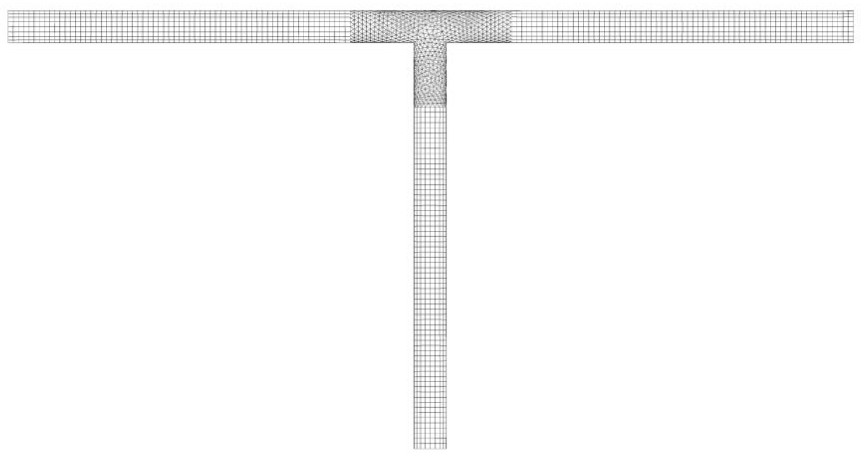
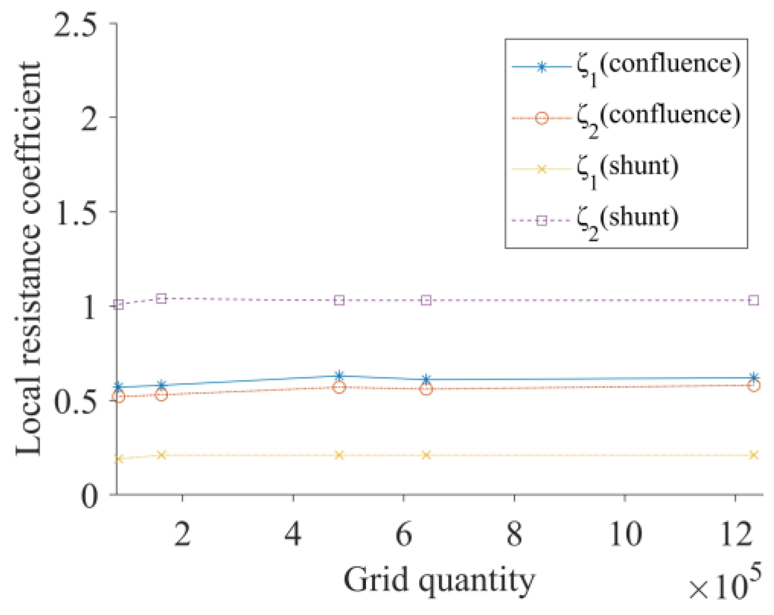
2.3. Grid Partitioning and Grid Independence Verification

The 3D grids were constructed with ANSYS ICEM. A hybrid grid system was employed, with hexahedral grids being used for the remaining portions and fine tetrahedral grids for the T-type part (Figure 4). Based on the traditional T-type tee model, the grid dependency was examined for the computational region shown in Figure 1a. Confluence and shunt conditions were tested for five structured grid schemes with the grid numbers 84,080, 161,622, 483,270, 640,675, and 1,233,451. Figure 5 displays the results of T-type tee local resistance coefficients ν1 and ζ₂, with a flow rate ratio of 0.5. It can be seen that the findings of both ζ₁ and ζ₂ became stable and essentially stayed unchanged if the grid number was higher than 483,270. For further simulation, a grid design with 483,270 cells was used. This system had a 0.1 mm first layer grid thickness, a 1.1 expansion ratio, and a y plus value between 60 and 270.

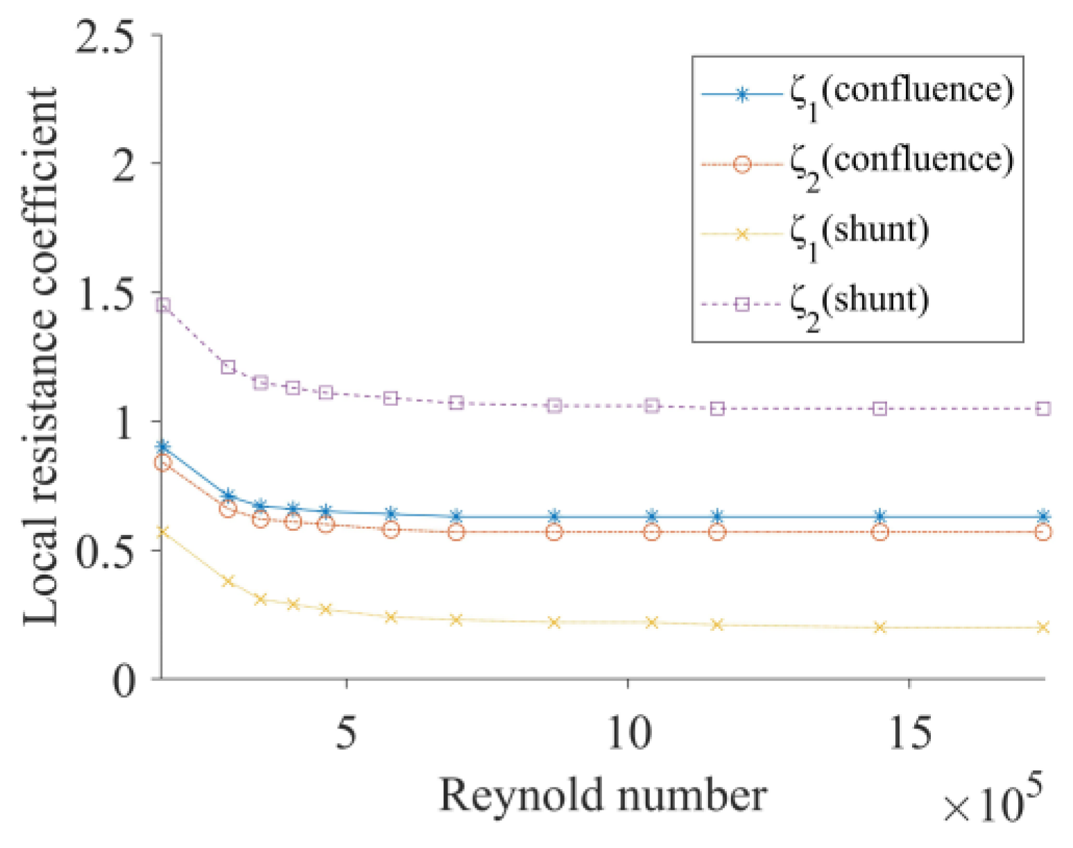
2.4. Model Validation

Model test validation was required to guarantee the accuracy of the numerical simulation results [35,36,37]. Northwest A&F University’s measurement data were used to validate the accuracy of the existing computer model [17]. Using a PVC confluence T-type tee as a base, the experiment measured the average pressure and flow rate of the cross sections for each branch. A frequency converter controlled the main pipe pressure, which ranged from 100 kPa to 300 kPa. It has been shown in prior studies that pipe flow validation results can be extended to a variety of diameter situations [18]. As a result, DN50 × 40 findings were used for validation. The measured data and the numerical results of the cross-sectional pressure were compared by applying the same computational domain and incoming flow circumstances. The average and maximum differences of P1 were 0.11% and 0.18%, respectively, as indicated in

Table 2. Comparison between numerical results and experimental data.

Boundary Condition			Numerical Results		Experimental Data		Error of P1/(%)	Error of P2/(%)
V1/(m·s−1)	V2/(m·s−1)	P3/Pa	P1/Pa	P2/Pa	P1 */Pa	P2 */Pa
0.30	1.65	119,345	121,013.9	120,833.6	121,203	121,106	0.16	0.22
0.37	1.71	140,768	142,685.8	142,472.3	142,920	142,920	0.16	0.31
0.44	1.73	163,855	165,975.8	165,739.6	166,105	166,202	0.08	0.28
0.51	1.75	185,865	188,164.8	187,912.4	188,408	188,506	0.13	0.31
0.57	1.80	207,386	209,943.0	209,662.1	210,027	210,125	0.04	0.22
0.65	1.83	233,114	235,926.6	235,622.6	236,342	236,440	0.18	0.35
0.75	1.72	249,646	252,473.5	252,202.4	252,483	251,896	0.01	0.12
0.83	1.78	270,091	273,252.8	272,955.9	273,613	273,026	0.13	0.03

Note: * means the experimental measured data.

. In contrast, P2 was 0.20% and 0.35%. These suggest that the existing numerical method for T-type tee local resistance prediction is adequately dependable.

3. Results and Discussion

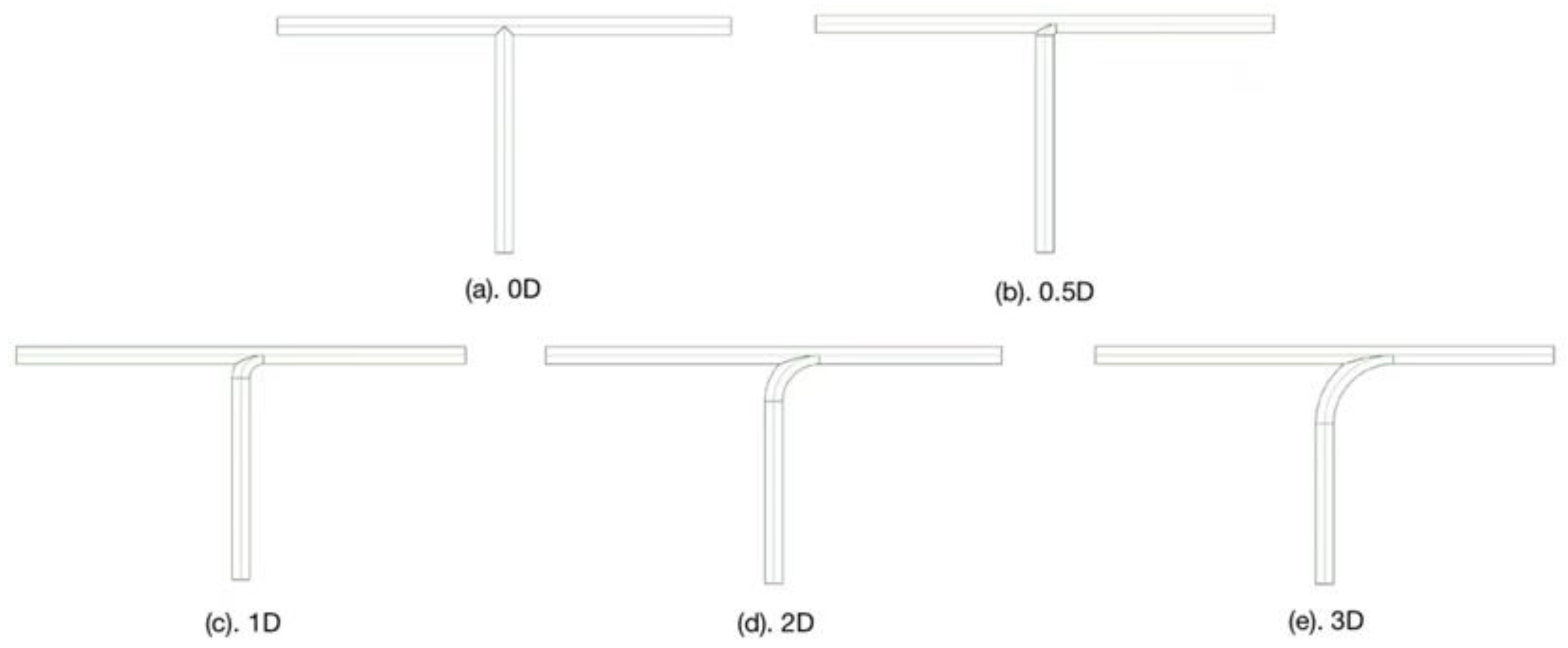
3.1. Effect of Chamfering Treatment on the T-Type Tee Flow Characteristics

3.1.1. Confluence

The most common case involves studying the flow characteristics of a T-type confluence tee using a flow rate ratio of 0.5 and five distinct chamfer radii (R = 0D, 0.5D, 1D, 2D, and 3D), all while maintaining the same main pipe diameter and side pipe. The Reynolds number for the numerical simulations was 868,648. In Figure 6, the streamline inside the tees is depicted, while Figure 7 presents a complete pressure contour at the axisymmetric plane of the T-type confluence tees with varying chamfer radii.

It is evident from Figure 6a that during the confluence process, the water flow in the side pipe will cause compression on the main pipe flow when the T-type tee’s chamfer radius is 0D. Consequently, there is an abrupt rise in flow velocity in the confluence area’s downstream section, particularly in the vicinity of the side pipe. This abrupt shift in flow velocity could be a major cause of energy loss. For T-type confluence tee performance, resistance optimization in the downstream region is therefore essential. When the streamline (Figure 6a) and total pressure (Figure 7a) are compared, it becomes clear that the classic T-type tee has a low-pressure backflow region downstream of the confluence area, particularly close to the side pipe, which causes a substantial amount of vortex flow. The decrease of flow resistance is made worse by this vortex flow.

After a thorough examination of Figure 6b–e and Figure 7b–e, it can be concluded that the flow pattern and pressure distribution inside the T-type confluence tee can be considerably changed by chamfering the tee. The side pipe flow’s influence on the main pipe flow diminishes with increasing chamfer radii. With time, the downstream velocity gradient at the main side pipe crossing becomes less pronounced. The process of wall detachment weakens as the low-pressure zone shrinks. Moreover, the vortex intensity decreases until it vanishes.

3.1.2. Shunt

The Reynolds number for the numerical simulations was 868,648. Figure 8 and Figure 9 show the streamline and total pressure distribution, respectively, of the axisymmetric plane of the T-type shunt tee with various chamfer radii. In traditional T-type shunt tees, a significant velocity and pressure gradient, as well as observable backflow and numerous vortices, can be seen downstream of the side pipe (Figure 8a). Vortices and wall separation are the main causes of flow energy loss.

A thorough examination of Figure 8b–e and Figure 9b–e shows that the fluid flow pattern and pressure distribution inside the T-type shunt tees can be significantly changed by chamfering the tees. The fluid in the main pipe can be redirected to the side pipe more readily and has less of an influence on the side pipe wall as the chamfer’s radius grows. Peak velocity drops as a result of a decrease in the velocity gradient in the side pipe’s downstream area. The phenomena of wall detachment weakens as the low-pressure region shrinks. Additionally, the numerous vortices subtly combine into a single vortex, and the vortex’s size and strength decreases.

3.2. Effect of Chamfering Treatment on Local Resistance Coefficient

3.2.1. Confluence

The Reynolds number for the numerical simulations was 868,648. Figure 10 displays the variation trend of the local resistance coefficients ζ₁ and ζ₂ under confluence conditions with various chamfer radii. Table 2 enumerates the particular values. Under confluence conditions, it was noted that the chamfering treatment efficiently reduces the local resistance loss of tees. The chamfer radius grows from 0D to 1D, which results in the greatest reduction in resistance. In contrast to the 0D situation, there is a 68% reduction in ζ₁ and an 82% reduction in ζ₂. The local resistance coefficients continue to fall as the chamfer radius increases, but the reduction rate also decreases. All of these findings suggest that the resistance reduction for confluence tees is not appreciably increased by chamfer radius increases beyond 1D. The best engineering practice for chamfering T-type confluence tees with a 1D radius of curvature may depend on relative elements including economic expenses, manufacturing processes, and application.

3.2.2. Shunt

The Reynolds number for the numerical simulations was 868,648. Figure 11 shows the variation trend of the local resistance coefficients ζ₁ and ζ₂ under shunt conditions with various chamfer radii. It is evident that, in shunt situations, the chamfering treatment also successfully lowered the local resistance loss of the tees. Compared to ζ₁, the chamfering procedure significantly reduced ζ₂. The reduction that happened most noticeably was when the chamfer radius went from 0D to 1D. In contrast to the 0D situation, there was a 24% and 54% reduction in ζ₁ and ζ₂, respectively. Both the reduction rate and the local resistance coefficients dropped as the chamfer radius increased. The optimal performance for practical uses was obtained by chamfering T-type shunt tees with a 1D radius of curvature, in line with the confluence results.

3.3. Crossed Effects of Chamfer Radius and Flow Rate Ratio

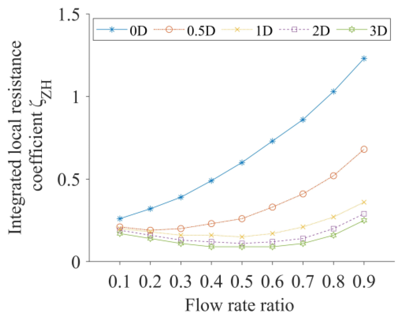
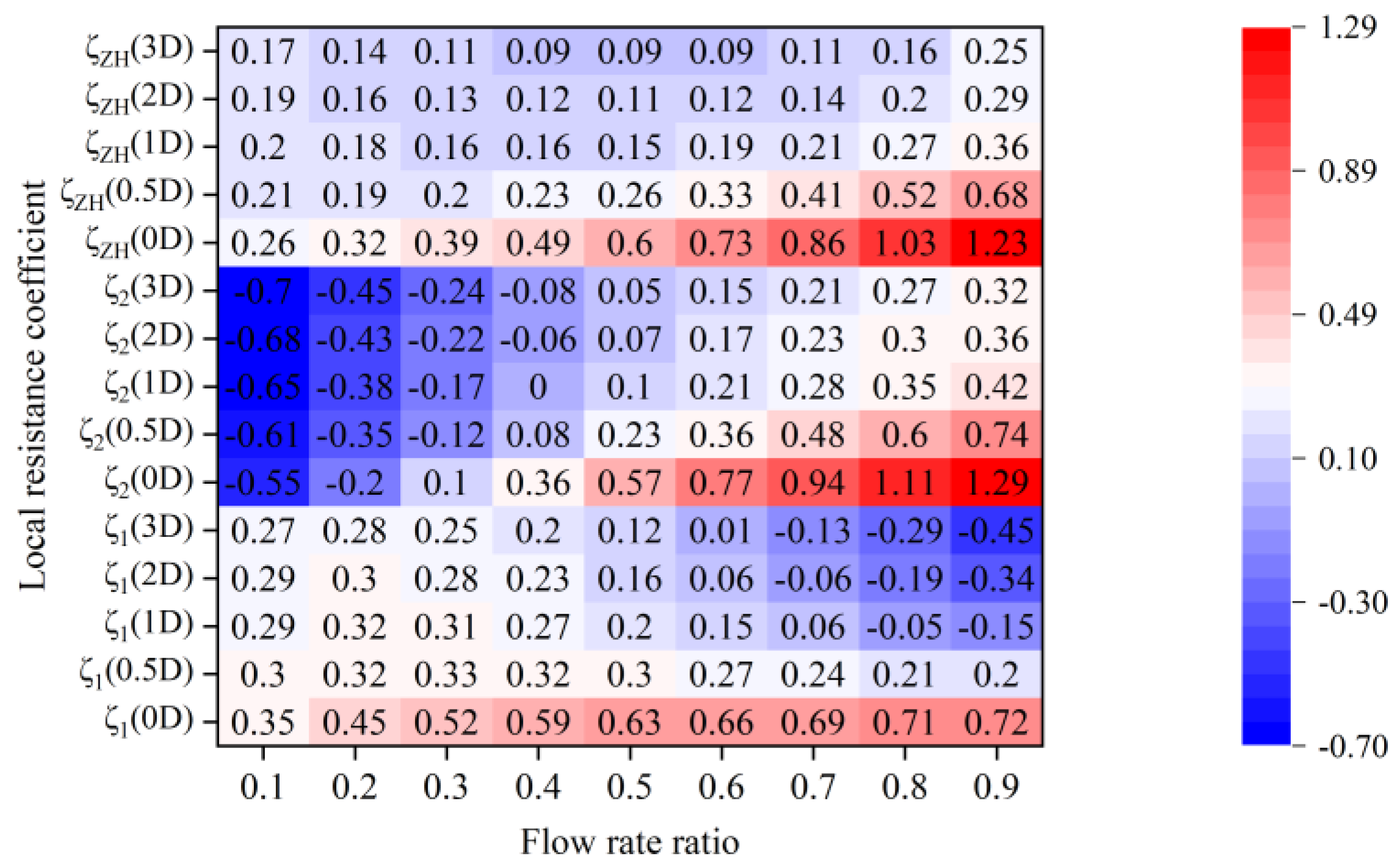
3.3.1. Confluence

The Reynolds number for the numerical simulations was 868,648. Under confluence conditions, Figure 12 shows the variation trend of the local resistance coefficients ζ₁ and ζ₂ with chamfer radius for various flow rate ratios (0.1, 0.2, 0.3, 0.4, 0.5, 0.6, 0.7, 0.8, and 0.9). It demonstrates that at most flow rate ratios, chamfering treatment can lower the local resistance loss under confluence conditions. Furthermore, a more noticeable decreasing impact is produced by a bigger chamfer radius and a higher flow rate ratio. The combined effects of energy loss from the collision at the main-side pipe intersection and energy exchanging due to the velocity difference between the two pipes determine the variation trend of the confluence tee local resistance coefficients ζ₁ and ζ₂ with the flow rate ratio.

The hydraulic characteristics were examined using the integrated local resistance coefficient ζZH in order to make a more straightforward comparison of the integral energy loss of T-type confluence tees with various flow rate ratios and chamfer radii possible. Figure 13 presents the results, and Figure 14 contains particular numerical data. A T-type confluence tee’s integrated local resistance coefficient can be successfully decreased in most cases by chamfering it. The resistance coefficient reduction becomes more significant as the flow rate ratio rises. Note that extending the chamfer radius further may not significantly boost the resistance reduction when the chamfer radius is more than 1D. The integrated local resistance coefficient under confluence shows a notable increase with the increasing flow rate ratio for chamfer radii of 0.5D and 0D, as can be seen from the fluctuation trend of the resistance coefficient with flow rate ratio. On the other hand, the integrated local resistance coefficient varies less with the flow rate ratio when the chamfer radius is greater than or equal to 1D. The findings show that, in addition to aiding in resistance reduction, chamfering a T-type tee with a chamfer radius equal to or more than 1D also helps pipe networks maintain resistance balance under variable flow conditions.

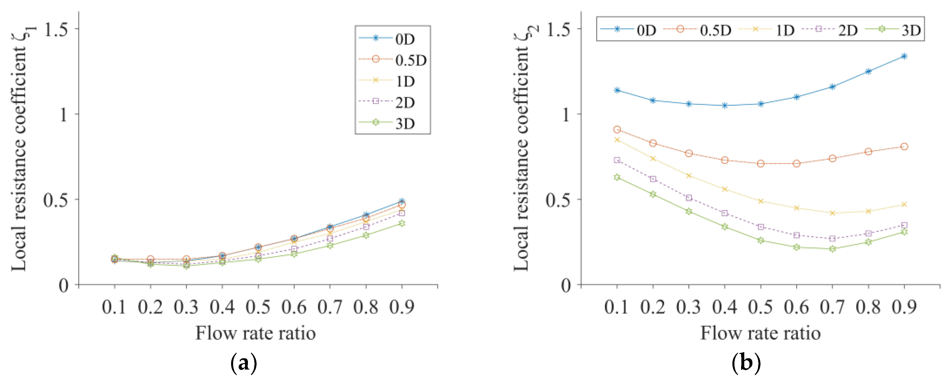
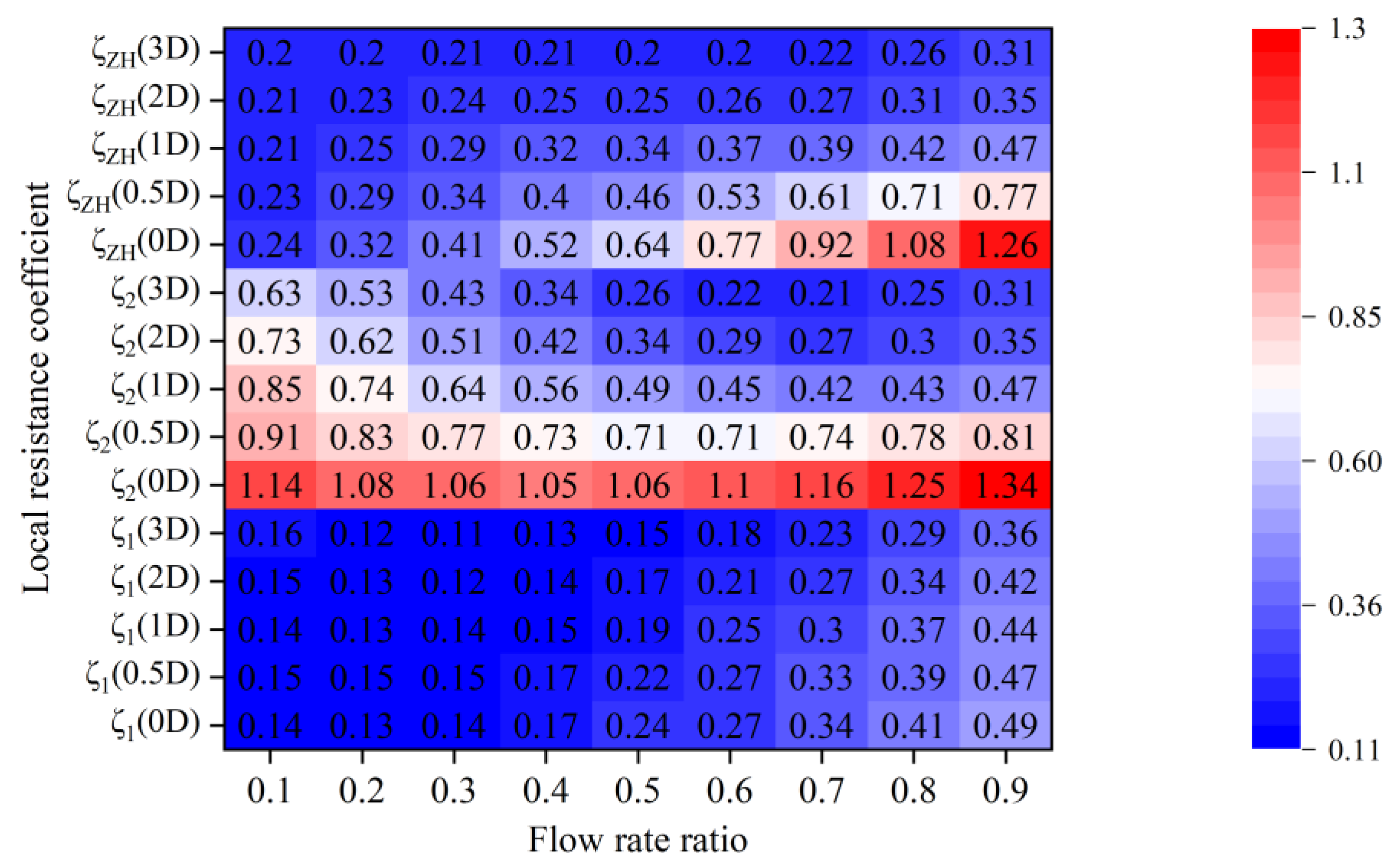
3.3.2. Shunt

The Reynolds number for the numerical simulations was 868,648. The trends of the local resistance coefficients ζ₁, ζ₂, and the integrated local resistance coefficient ζ_ZH with chamfer radius are shown in Figure 15 and Figure 16, respectively, and the specific values are shown in Figure 17; in the case of a shunt, under different flow rate ratios (0.1, 0.2, 0.3, 0.4, 0.5, 0.6, 0.7, 0.8, and 0.9). T-type shunt tees can benefit from chamfering treatment to minimize local resistance loss under most flow rate ratios, similar to confluence situations. A more pronounced reduction impact is achieved by increasing the chamfer radius and increasing the flow rate ratio.

3.4. Crossed Effects of Chamfer Radius and Pipe Diameter Ratio

According to the analysis above, chamfering treatment can successfully lower tees’ local resistance loss at the same diameter. To achieve comparable flow velocities in the main and side pipes, however, differing diameter tees are frequently utilized in practical applications of liquid transmission and distribution. It is necessary to perform a crossed-effect analysis of the chamfer radius and pipe diameter ratio in order to investigate the resistance reduction impact of chamfering treatment under various pipe diameter ratios.

A good resistance reduction has been demonstrated to be achievable with a chamfer radius of 1D. Thus, two groups of commonly used T-type tees with 1D chamfer radii and main pipe sizes of 110 mm and 160 mm are accepted in this paragraph. This is to look at how chamfering treatment affects resistance reduction when the pipe diameter ratio changes.

3.4.1. Confluence

The main side pipe’s input velocity was set to 2 m/s, with a Reynolds number of ≥386,066. The main side pipe’s flow rate ratio varied in tandem with changes in the pipe diameter ratio. Therefore, the total resistance effect of the tee is represented by the integrated local resistance coefficient. For the two groups of tees with main pipe diameters of 110 mm and 160 mm, Figure 18 shows the progression of the integrated local resistance coefficient ζ_ZH with the pipe diameter ratio. The strength of the chamfering treatment’s resistance reduction impact is indicated by the distance between the 0D and 1D lines.

It is noted that the resistance reduction effect of the chamfering treatment was weak when the pipe diameter ratio was less than 0.5. Nonetheless, the resistance reduction effect progressively became stronger as the pipe diameter ratio rose. The integrated local resistance coefficient decreased by more than 60% when the pipe diameter ratio approached 0.5, demonstrating a notable resistance reduction effect. The resistance decrease increased with the pipe diameter ratio for ratios larger than or equal to 0.7, although at a slower rate. Figure 19 displays the integrated local resistance coefficient values for various pipe diameter ratios and the chamfer radii during confluence conditions.

3.4.2. Shunt

The main side pipe’s input velocity was set to 2 m/s, with a Reynolds number of ≥386,066. For shunt instances, Figure 20 shows the trend of the integrated local resistance coefficient ζ_ZH with the pipe diameter ratio; Figure 21 provides the specific values. Comparable to the confluence situations, when the pipe diameter ratio was less than 0.5, the resistance reduction effect of the chamfering treatment under shunt conditions was less pronounced. Nonetheless, the resistance reduction effect progressively became stronger as the pipe diameter ratio rose. It is shown that the resistance reduction impact increased with pipe diameter ratio up to 0.5.

In conclusion, when the pipe diameter ratio was more than 0.5, chamfering treatment with a 1D radius of curvature significantly reduced resistance in actual applications when the main and side pipe entrance velocities were similar. Nonetheless, the chamfering treatment’s resistance-reduction effect was comparatively smaller when the pipe diameter ratio was less than 0.5.

4. Conclusions

Under confluence and shunt situations, the optimization and resistance reduction impacts of chamfering treatment on T-type tee flow characteristics were studied, taking into account the ratios of pipe diameter to flow rate. A numerical technique with experimental validation was used. The findings of this study can be summed up as follows:

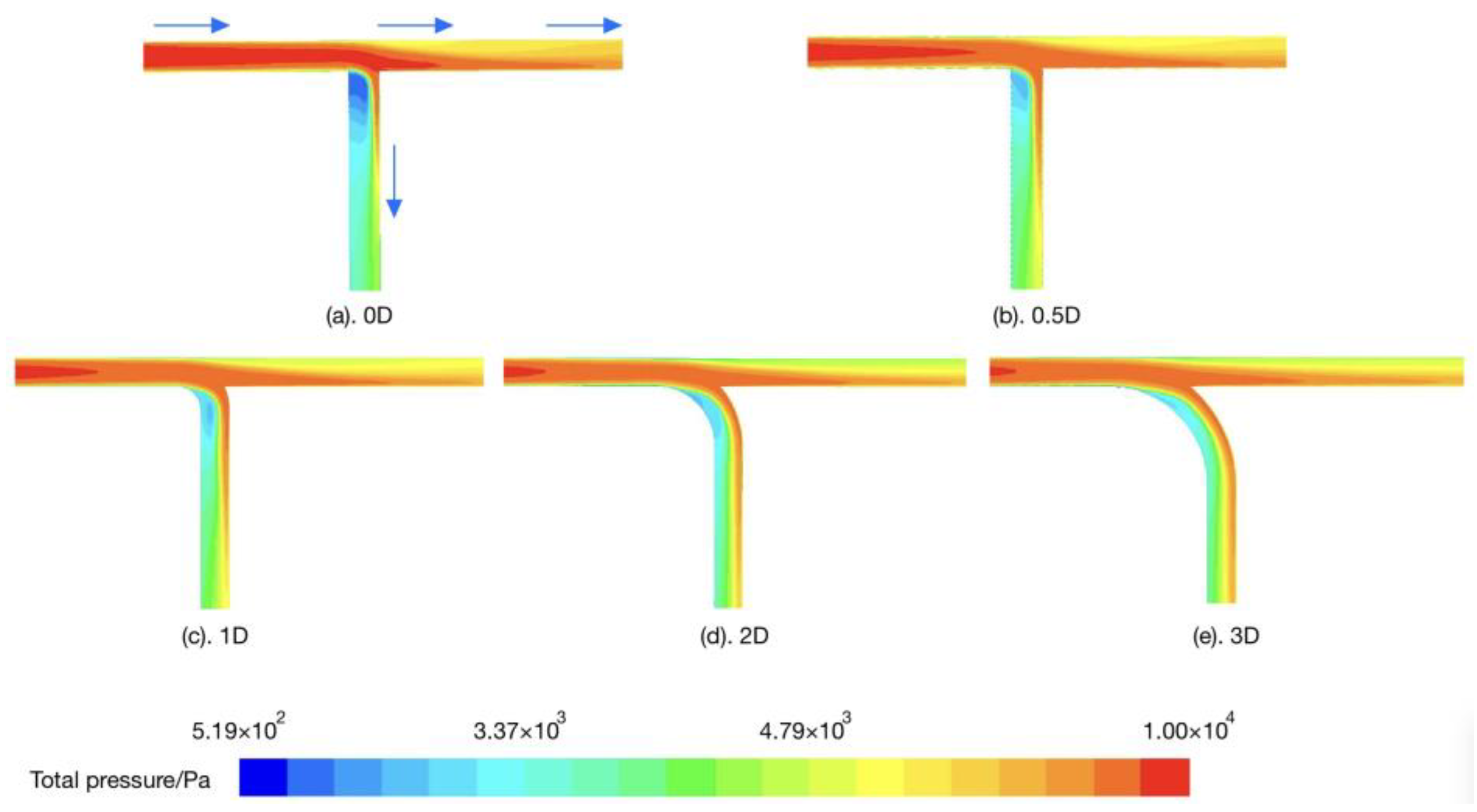
• For the confluence tees, the side pipe flow compressed the main pipe flow, which caused an abrupt increase in flow velocity in the downstream area and a large loss of energy. Vortices and wall detachment were the main causes of flow energy loss in the shunt tees. By decreasing velocity gradients, limiting velocity direction changes, and lessening vortex strength, chamfering the T-type tee can significantly improve the flow field under both confluence and shunt situations.
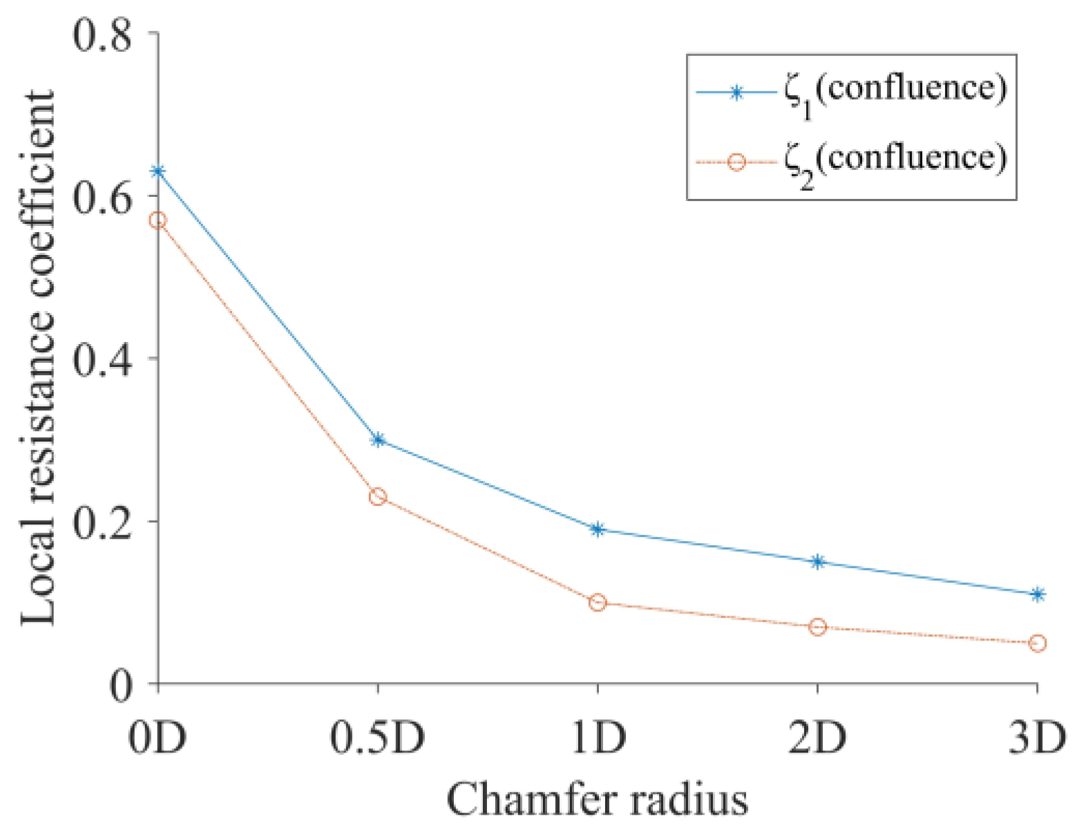
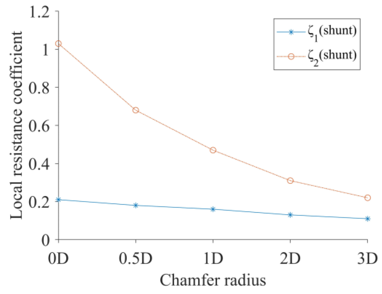
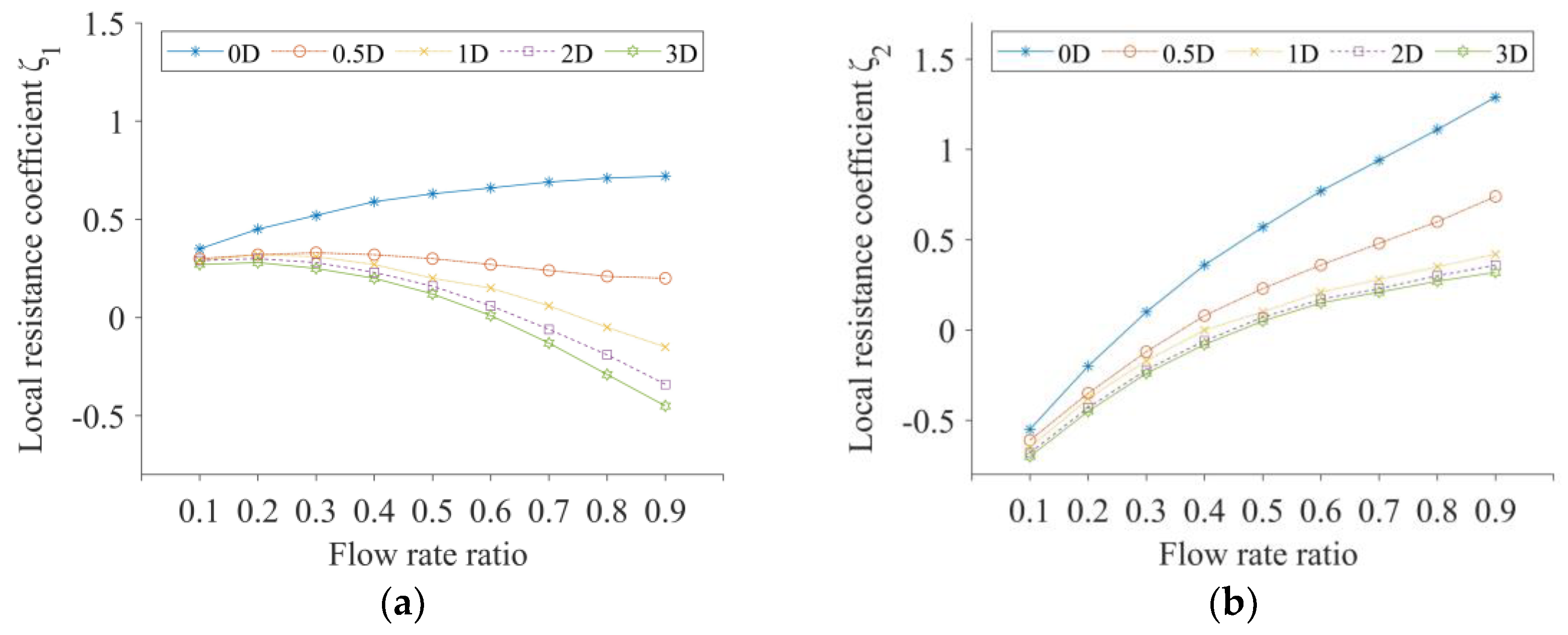
• As the flow rate ratio and chamfer radius increased, the resistance reduction impact of the chamfering treatment on the T-type tee became more noticeable.
• Chamfering T-type tees with chamfer radii equal to or larger than 1D helped maintain resistance balance for pipe networks under varying flow circumstances in addition to aiding in resistance reduction. Under practical engineering conditions, the chamfering treatment of a T-type confluence tee with a 1D radius of curvature may be the best option when taking into account related elements like manufacturing processes, economic expenses, and applicability.
• When the pipe diameter ratio was more than 0.5, the chamfering treatment resulted in a greater resistance reduction for unequal tees with equivalent velocities in the main and side pipes.

This paper provides reference data on the local resistance coefficients of the tee under various combinations of different chamfer radius, flow rate ratios, and pipe diameter ratios. It methodically researched the effects of chamfer radius on the local resistance characteristics of T-type tee under confluence and shunt conditions. Despite existing limitations, the novel insights unveiled in this investigation can enhance comprehension of the local resistance attributes of T-type tees in both confluence and shunt scenarios. In order to compensate for the existing dearth of reference data on the local resistance coefficients of T-type tees, it offers useful support data on the local resistance coefficients of the tee under various combinations of varied chamfer radii, flow rate ratios, and pipe diameter ratios. The design of liquid transmission and distribution systems may both benefit from these findings, which also have the potential to lower carbon emissions and save energy. The application of these findings could improve the sustainability of the manufacturing and operation processes.

References

- Yu, C.; Wang, Q.; He, J.; Li, H.; Lu, C.; Liu, Z. Development of spraying device for precise and deep application of liquid fertilizer in sowing period. Trans. Chin. Soc. Agric. Eng. 2019, 35, 50–59, (In Chinese with English Abstract). [Google Scholar] [CrossRef]
- Xue, X.; Zhang, B.; Zhang, Z.; Lin, D.; Song, S.; Li, Z.; Hong, T. Design and experiment of variable liquid fertilizer applicator for deep-fertilization based on ZigBee technology. J. Drain. Irrig. Mach. Eng. 2020, 38, 318–324, (In Chinese with English Abstract). [Google Scholar]
- Li, T.; Li, J.C.; Wu, J.L.; Zhang, B.B.; Lu, J.F. Design and Experiment of Bypass Fertilizer-type. Water and Fertilizer Integrated Automatic Fertilizer Applicator. Water Sav. Irrig. 2018, 98–102, 106, (In Chinese with English Abstract). [Google Scholar]
- Ozkahraman, H.T.; Bolatturk, A. The use of tuff stone cladding in buildings for energy conservation. Constr. Build. Mater. 2006, 20, 435–440. [Google Scholar] [CrossRef]
- Lu, H.; Pei, G.; Yang, L. Hydraulics; China Agriculture Press: Beijing, China, 2002. [Google Scholar]
- GB/T50485—2020; Technical Standard for Microirigation Engineerin. China Planning Press: Beijing, China, 2020.
- Shi, X.; Lü, H.; Zhu, D.; Sun, B.; Cao, B. Flow Resistance and Characteristics of PVC Tee Pipes. Trans. Chin. Soc. Agric. Mach. 2013, 44, 73–79, 89, (In Chinese with English Abstract). [Google Scholar] [CrossRef]
- Pérez-García, J.; Sanmiguel-Rojas, E.; Viedma, A. New experimental correlations to characterize compressible flow losses at 90- degreeT-unctions. Exp. Therm. Fluid Sci. 2009, 33, 261–266. [Google Scholar] [CrossRef]
- Pérez-García, J.; Sanmiguel-Rojas, E.; Hernández-Grau, J.; Viedma, A. Numerical and experimental investigations on internal comoressible flow at T-ypejunctions. Exp. Therm. Fluid Sci. 2006, 31, 61–74. [Google Scholar] [CrossRef]
- Gong, Q.; Yang, J.; Han, K.; Huang, T.; Li, J.; Zuo, P. Characteristic Analysis on the Flow and Local Resistance in Large Pipe Tees. J. Chin. Soc. Power Eng. 2020, 36, 753–764, (In Chinese with English Abstract). [Google Scholar] [CrossRef]
- Chen, W.; Lv, H.; Shi, X.; Zhou, J. Experimental Study on Local Loss Parameter of Diameter PVC Pipe Tee. J. Irrig. Drain. 2013, 32, 128–130, (In Chinese with English Abstract). [Google Scholar]
- Shi, X.; Tao, H.; Chai, Y.Y.; Wan, B.Q. Numerical Simulation of Resistance Loss and Flow Characteristics on UPVC Slope Tee Pipes. China Rural Water Hydropower 2018, 11, 170–174, (In Chinese with English Abstract). [Google Scholar] [CrossRef]
- Shang, X.; Ji, R. Visual analysis of resistance characteristics and flow field of manifold tee pipe based on CFD. Sci. Tech. Inf. Gansu 2021, 50, 25–28. (In Chinese) [Google Scholar]
- Xu, H.; Wu, W.; Wang, Z.; Wang, Q. Hydraulic characteristics analysis and flow field calculation of inclined tee pipes based on CFD. J. Drain. Irrig. Mach. Eng. 2020, 38, 1138–1144, (In Chinese with English Abstract). [Google Scholar]
- Zhou, G. Oblique tee in-pipe flow simulation. Energy Conserv. 2021, 12, 47–49, (In Chinese with English Abstract). [Google Scholar] [CrossRef]
- Zhang, Q.; Zhang, M.; Zhou, Z.; Wei, S. Numerical Calculation of the Tee Local Resistance Coefficient. Open Mech. Eng. J. 2015, 9, 876–881. [Google Scholar] [CrossRef]
- Zhu, J.; Bo, Y.; Zhu, D.; Li, J.; Zheng, C.; Gao, F. Numerical Simulation and Experimental Study on Hydraulic Characteristics of Fertilizer Injection Tee Pipe. J. Water Resour. Archit. Eng. 2021, 19, 134–138, (In Chinese with English Abstract). [Google Scholar] [CrossRef]
- Chen, J.; Lü, H.; Shi, X.; Zhu, D.; Wang, W. Numerical simulation and experimental study on hydrodynamics characteristics of T-type pipes. Trans. Chin. Soc. Agric. Eng. 2012, 28, 73–77, (In Chinese with English Abstract). [Google Scholar] [CrossRef]
- Kalenik, M.; Chalecki, M.; Wichowski, P. Real Values of Local Resistance Coefficients during Water Flow through Welded Polypropylene T-Junctions. Water 2020, 12, 895. [Google Scholar] [CrossRef]
- Sharp, Z.B.; Johnson, M.C.; Barfuss, S.L.; Rahmeyer, W.J. Energy losses in cross junctions. ASCE J. Hydraul. Eng. 2010, 136, 50–55. [Google Scholar] [CrossRef]
- Weitbrecht, V.; Lehmann, D.; Richter, A. Flow distribution in solar collectors with laminar flow conditions. Sola Energy 2003, 73, 433–441. [Google Scholar] [CrossRef]
- Gan, G.; Riffat, S.B. Numerical determination of energy losses at duct junctions. Appl. Energy 2000, 67, 331–340. [Google Scholar] [CrossRef]
- Costa, N.P.; Maia, R.; Proença, M.F.; Pinho, F.T. Edge effects on the flow characteristics in a 90 deg tee junction. ASME J. Fluids Eng. 2006, 128, 1204–1217. [Google Scholar] [CrossRef]
- Ammarullah, M.I.; Hartono, R.; Supriyono, T.; Santoso, G.; Sugiharto, S.; Permana, M.S. Polycrystalline Diamond as a Potential Material for the Hard-on-Hard Bearing of Total Hip Prosthesis: Von Mises Stress Analysis. Biomedicines 2023, 11, 951. [Google Scholar] [CrossRef]
- Salaha, Z.F.M.; Ammarullah, M.I.; Abdullah, N.N.A.A.; Aziz, A.U.A.; Gan, H.-S.; Abdullah, A.H.; Abdul Kadir, M.R.; Ramlee, M.H. Biomechanical Effects of the Porous Structure of Gyroid and Voronoi Hip Implants: A Finite Element Analysis Using an Experimentally Validated Model. Materials 2023, 16, 3298. [Google Scholar] [CrossRef]
- Lamura, M.D.P.; Hidayat, T.; Ammarullah, M.I.; Bayuseno, A.P.; Jamari, J. Study of contact mechanics between two brass solids in various diameter ratios and friction coefficient. Proc. Inst. Mech. Eng. Part J J. Eng. Tribol. 2023, 237, 14657503221144810. [Google Scholar] [CrossRef]
- Xu, Q. Resistance Characteristic Andreduction Analysis of T-Type Tee under Different Intersection Angles. Master’s Thesis, Shandong Jianzhu University, Jinan, China, 2022. (In Chinese with English Abstract). [Google Scholar]
- Sahin, A.Z.; Kalyon, M. Maintaining uniform surface temperature along pipes by insulation. Energy 2005, 30, 637–647. [Google Scholar] [CrossRef]
- Chen, X. Calculation model research of local resistance coefficient for spacer grids based on CFD methodology. At. Energy Sci. Technol. 2016, 50, 277–281, (In Chinese with English Abstract). [Google Scholar] [CrossRef]
- Wang, F. Computational Fluid Dynamics Analysis: Principles and Applications of CFD Software; Tsinghua University Press: Beijing, China, 2004. (In Chinese) [Google Scholar]
- Zhu, H.; Lin, Y.; Xie, L. FLUENT Fluid Analysis Engineering Case Introduction; Publishing House of Electronics Industry: Beijing, China, 2013. (In Chinese) [Google Scholar]
- Austin, R.G.; Waanders, B.v.B.; McKenna, S.; Choi, C.Y. Mixing at Cross Junctions in Water Distribution Systems. II: Experimental Study. J. Water Resour. Plan. Manag. 2008, 134, 295–302. [Google Scholar] [CrossRef]
- Renberg, U.R.; Westin, F.; Angstrom, H.-E.; Fuchs, L. Study of Junctions in 1-D & 3-D Simulation for Steady and Unsteady Flow. Sae Tech. Pap. 2010, 33, 261–266. [Google Scholar] [CrossRef]
- Hua, S.; Yang, X. Practical Fluid Resistance Manual; National Defense Industry Press: Beijing, China, 1985. (In Chinese) [Google Scholar]
- Lamura, M.D.P.; Ammarullah, M.I.; Hidayat, T.; Maula, M.I.; Jamari, J. Diameter ratio and friction coefficient effect on equivalent plastic strain (PEEQ) during contact between two brass solids. Cogent Eng. 2023, 10, 1. [Google Scholar] [CrossRef]
- Jamari, J.; Ammarullah, M.I.; Santoso, G.; Sugiharto, S.; Supriyono, T.; Permana, M.S.; Winarni, T.I.; van der Heide, E. Adopted walking condition for computational simulation approach on bearing of hip joint prosthesis: Review over the past 30 years. Heliyon 2022, 8, 1241. [Google Scholar] [CrossRef]
- Jamari, J.; Ammarullah, M.I.; Santoso, G.; Sugiharto, S.; Supriyono, T.; van der Heide, E. In Silico Contact Pressure of Metal-on-Metal Total Hip Implant with Different Materials Subjected to Gait Loading. Metals 2022, 12, 1241. [Google Scholar] [CrossRef]