What Are the Correlations between Human Disturbance, the Spatial Pattern of the Urban Landscape, and Eco-Environmental Quality?

Abstract

Human transformation of the landscape is reflected in its composition and spatial pattern. Therefore, exploring the response of the eco-environment to the composition and spatial pattern of the landscape is beneficial to providing a theoretical basis for urban planners. In this study, we take a typical oil city in China as an example and introduce the hemeroby index, landscape metrics, and a remote sensing-based ecological index (RSEI) to calculate and evaluate the urban landscape pattern, human disturbance, and eco-environmental quality, as well as exploring the relationships between them. The results demonstrate that the mean RSEI value of the study area was 0.4866, indicating that its eco-environmental quality was relatively moderate. The whole study area had a relatively high degree of human disturbance (hemeroby index = 7.4498), where the effect of human disturbance on the eco-environment was more intense in natural ecosystems, such as forest and grasslands, but less intense in artificial landscapes, such as built-up areas and farmlands. The urban landscape pattern was significantly correlated with eco-environmental quality, among which the proportion of green space and impervious surface had the strongest correlations with the mean RSEI, with correlation coefficients of 0.538 and −0.577, respectively. In addition, the correlation between the landscape pattern and the RSEI presented obvious spatial heterogeneity.

1. Introduction

Over the past decades, the natural landscape has been modified into agricultural, industrial or urban development and construction land all over the world [1,2,3]. To meet the increasing demand for natural resources, human activities have covered entire areas of the planet, transforming 30–50% of the earth’s ecological surface system through a great deal of different means [4,5,6,7]. Except for the natural succession of different land types, landscape compositions, landscape patterns, and abundant landscape management policies are not only the trace of human transformation of nature’s landscape, but comprise the most intuitive manifestation of human disturbances [8,9,10]. Therefore, research on the ecological effects of landscape composition and patterns has gradually become a hot topic of research in ecology, geography, environmental science, architecture, and other related disciplines, providing a theoretical basis for promoting the sustainable green development of the global ecological system [11,12,13,14].

The application of remote sensing technology has recently become a key scientific measure for the evaluation of regional eco-environmental quality; in this line, many studies have successfully combined various ecological indicators with the characteristics of landscape composition and pattern [15,16,17,18,19]. For instance, a variety of studies have explored the relationship between the landscape spatial pattern and the urban heat island (UHI) effect with the help of land surface temperature (LST) [20,21,22,23,24]; furthermore, some studies have explored the impact of land expansion on regional plant species diversity and hydrology [25,26]. However, most previous studies paid more attention to the effect of landscape structure on certain features of the ecological environment. Based on this, Xu [27] invented a new remote sensing-based ecological index (RSEI), which integrates the primary indicators of ecological environment features (i.e., land surface temperature, degree of dryness, green space coverage, and land surface moisture) in order to evaluate the urban ecological quality. Subsequently, the RSEI has been widely applied in various fields of environmental research. Wen et al. [28] and Qureshi et al. [29] provided general assessments of eco-environmental quality at the urban level through monitoring the changes in the RSEI. Yue et al. [30] and Zheng et al. [31] monitored and studied the dynamics of eco-environmental quality at a larger scale (e.g., China’s 35 major cities and coastal zones). Shan et al. [32] identified the spatiotemporal dynamic change in the RSEI in different periods of land consolidation in order to explore the effects of land development intensity on the eco-environmental quality. With a moving window-based RSEI, Zhu et al. [33] assessed the impacts of opencast mining on the eco-environmental quality. Ariken et al. [34] established a coupling coordination degree model to analyze the coupling degree between urbanization and eco-environmental quality. Gone et al. [35] used the RSEI to explore the spatiotemporal variations in the eco-environment quality and the effects of different influencing factors on the RSEI changes during 2000–2020 based on geo-detection. Yang et al. [36] adopted the RSEI to evaluate the ecological quality of Hangzhou Bay Area, China, and discussed the impact of LUCC on it. Zhang et al. [37] analyzed the eco-environmental quality in the Chang–Zhu–Tan metropolitan circle, central China, during 2000–2020 based on Google Earth Engine (GEE) and the RSEI, and explored the response of the RSEI to the direct and indirect effects of natural and anthropogenic factors. However, there have not been as many studies focused on the impact of the regional landscape spatial pattern on eco-environmental quality [10,38,39,40]; in particular, there have been relatively few studies using the RSEI to explore these effects. Hence, in this study, we pay more attention to the impact of landscape spatial pattern and composition on the eco-environmental quality, according to the RSEI.

The effect of human disturbance on the natural environment system is reflected in the landscape composition; as such, it is necessary to construct a human disturbance index that contains landscape composition-related information, in order to study its effect on the eco-environmental quality [41,42]. The German ecologist Sukopp [43] proposed the conception of “Hemeroby,” which was initially adopted to describe the effects of human disturbance on vegetation systems, as a measure to assess the naturalness of flora [44,45,46,47,48]. Later, it was applied to assess the degree of human disturbance on ecosystems and ecological environments [49,50,51]. In recent years, through assigning hemeroby weights to each landscape type, some studies have transformed different landscape types into synthetic values to represent the degree of human interference [52,53,54,55,56]. Compared with previous studies, which investigated socio-economic, political, and cultural factors to reflect human interference [57,58,59], these studies calculated the degree of human interference from the perspective of physical geography through the use of remote sensing techniques and other spatial analysis technology. Therefore, it is significantly important to explore the effect of human activities on the ecological environment by adopting the concept of hemeroby at a variety of scales, instead of simply using field investigation information and national statistic gazette documents [7,42,60,61]. For example, Zhao et al. [62] explored the heterogeneity of wetland landscapes and their relationships with anthropogenic disturbances and precipitation in a semi-arid region of China, based on the hemeroby index. Jasinaviciute and Veteikis [63] evaluated the landscape instability of Lithuanian LUCC based on the hemeroby index. However, previous studies have often used the hemeroby index to evaluate the intensity of human disturbance of landscape and its impact on landscape pattern, while lacking discussion on its relationship with eco-environmental quality.

For this study, we selected a city in northeastern China with perennial human intervention due to the exploitation of natural resources as an example, and introduced landscape metrics and two synthetic indicators (i.e., RSEI and hemeroby), in order to calculate the landscape pattern and the intensity of human disturbance, and evaluate the eco-environmental quality of the study area, as well as to conduct an innovative study on the relationships between these indicators and explore the effects of spatial differentiation on these relationships. On the basis of the above, we hope to solve the following research questions: (1) How can we use remote sensing data and other spatial statistic methods to quantify the eco-environmental quality and the degree of human interference at a regional scale? (2) What are the effects of different hemeroby levels on the eco-environmental quality in the study area? and (3) What is the relationship between the spatial landscape pattern of the study area and the eco-environmental quality? The results of this study are expected to enrich the theoretical basis regarding landscape configuration in regional landscape planning, as well as promoting the development of the ecological environment to a better condition by adjusting and controlling the urban landscape composition and spatial pattern.

2. Materials and Methods

2.1. Study Area

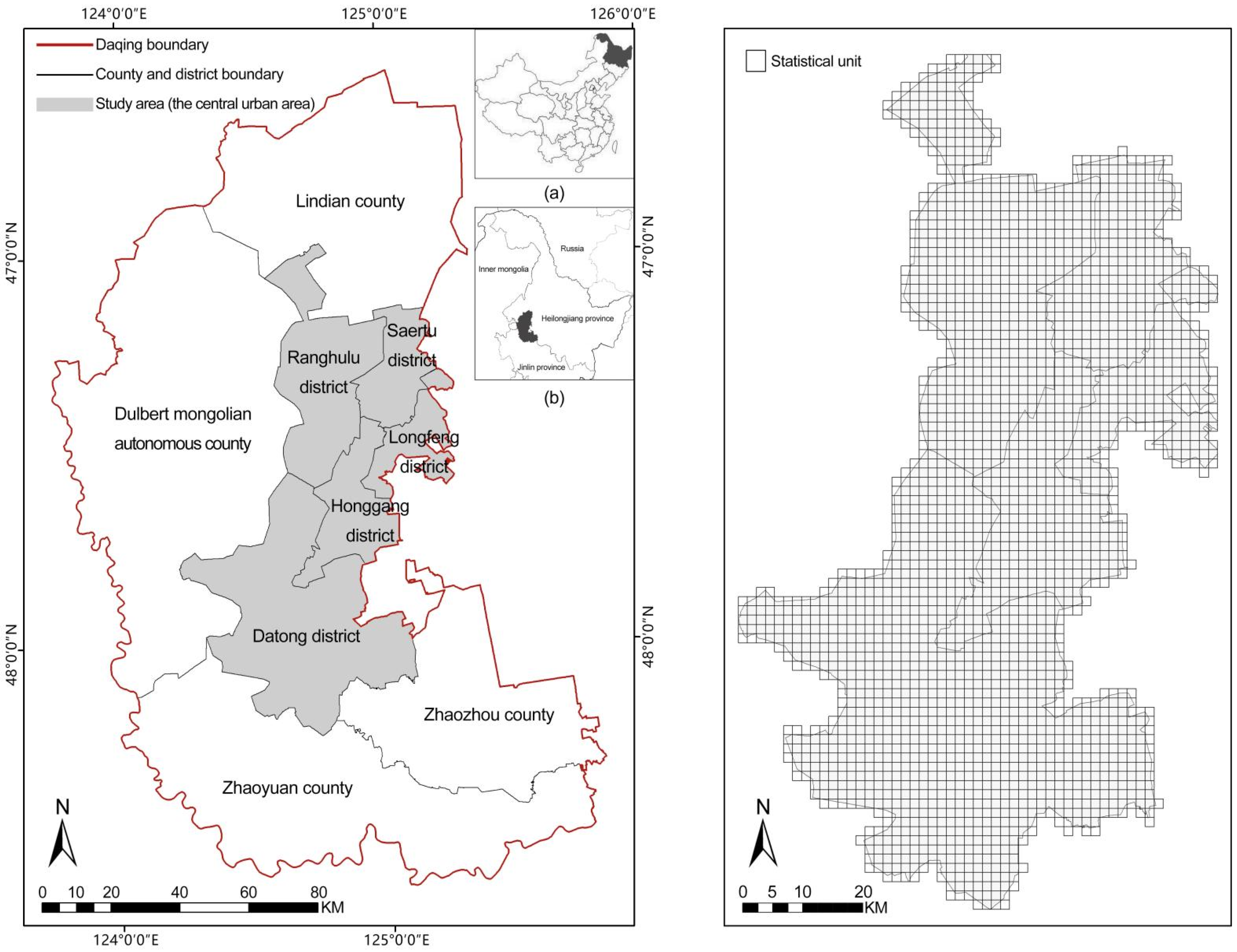
The study area is located in the center of Daqing City, Heilongjiang Province, China, which is a resource-based city, with petroleum exploitation and processing as its main industry (45°22ʹ–47°30ʹ N, 123°44ʹ–125°48 E; see Figure 1). With a flat terrain and four distinctive seasons, its annual mean temperature and rainfall are 4.2 ℃ and 427.5 mm, respectively. The study area is not only the largest oil field in China, but is also rich in cultivated land resources, natural wetlands, and meadows of different sizes. However, over the years, with the continuous depletion of resources and the growth of the population, the natural ecological land has been occupied to meet the growing social and economic needs and, so, the quality of the urban ecological environment has been declining [64].

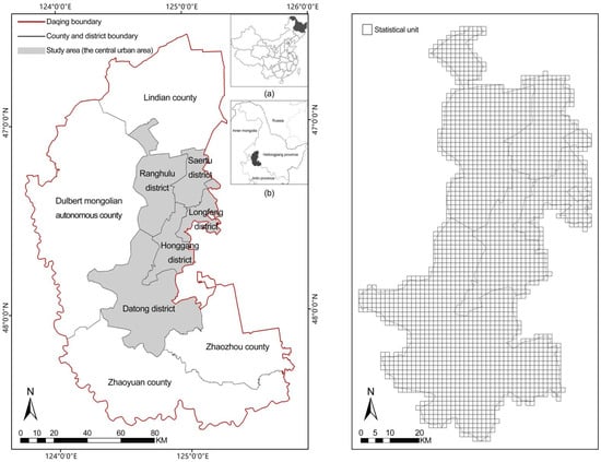
Figure 1. Location of the study area (left) and the distribution of statistical grids (right), and the size of statistical grid is 1.5 km × 1.5 km, with a total of 2481. (a) The location of the province where the study area is located in China; (b) the location of the city where the study area is located in the province.

According to previous studies, “the area of a statistical unit should be 2–5 times of the mean patch area. In this way, the landscape pattern of the statistical unit can be expressed more clearly”. [65] Through calculation, the mean patch area of the study area was 0.5962 km², based on the resolution of the remote sensing imagery and our research needs; thus, we divided the study area into 2481 statistical units, with each unit measuring 1.5 km × 1.5 km (Figure 1).

2.2. Image Processing

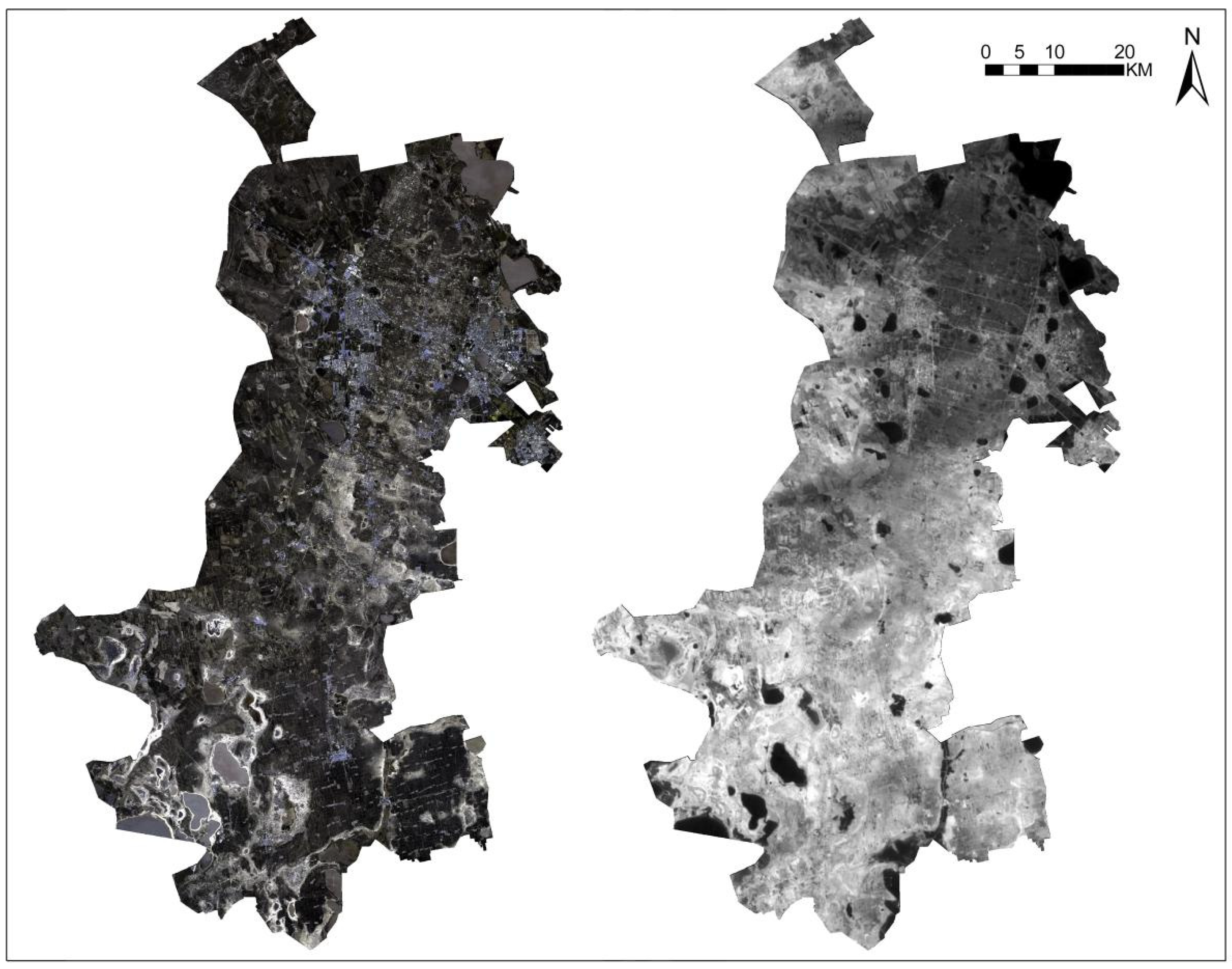
Since the study area has four distinct seasons, its eco-environmental quality has great differences in different seasons. The eco-environmental quality in this area is relatively good from June to September, as the vegetation growth is vigorous during this period. Therefore, we adopted Landsat-8 OLI and TIRS images, obtained on 6 September 2019, from the United States Geological Survey (USGS; https://glovis.usgs.gov/ (accessed on 5 June 2022)) to conduct research under the background of good eco-environmental quality in the study area. To fully cover the entire study area, two scenes of images with path/row numbers of 119/27 and 119/28 with a spatial resolution of 30_m were adopted. Figure 2 shows the remote sensing images after using the mask of the study area boundary. Meanwhile, two LULC classification methods (i.e., supervised classification and spectral index-based methods) were employed, in preparation for calculating the hemeroby and the effect of the landscape pattern on the RSEI.

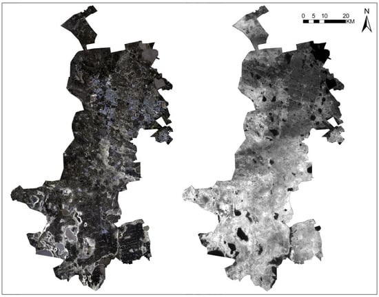
Figure 2. Original Landsat-8 images of the study area. The left one is OLI image and the right one is TIRS image.

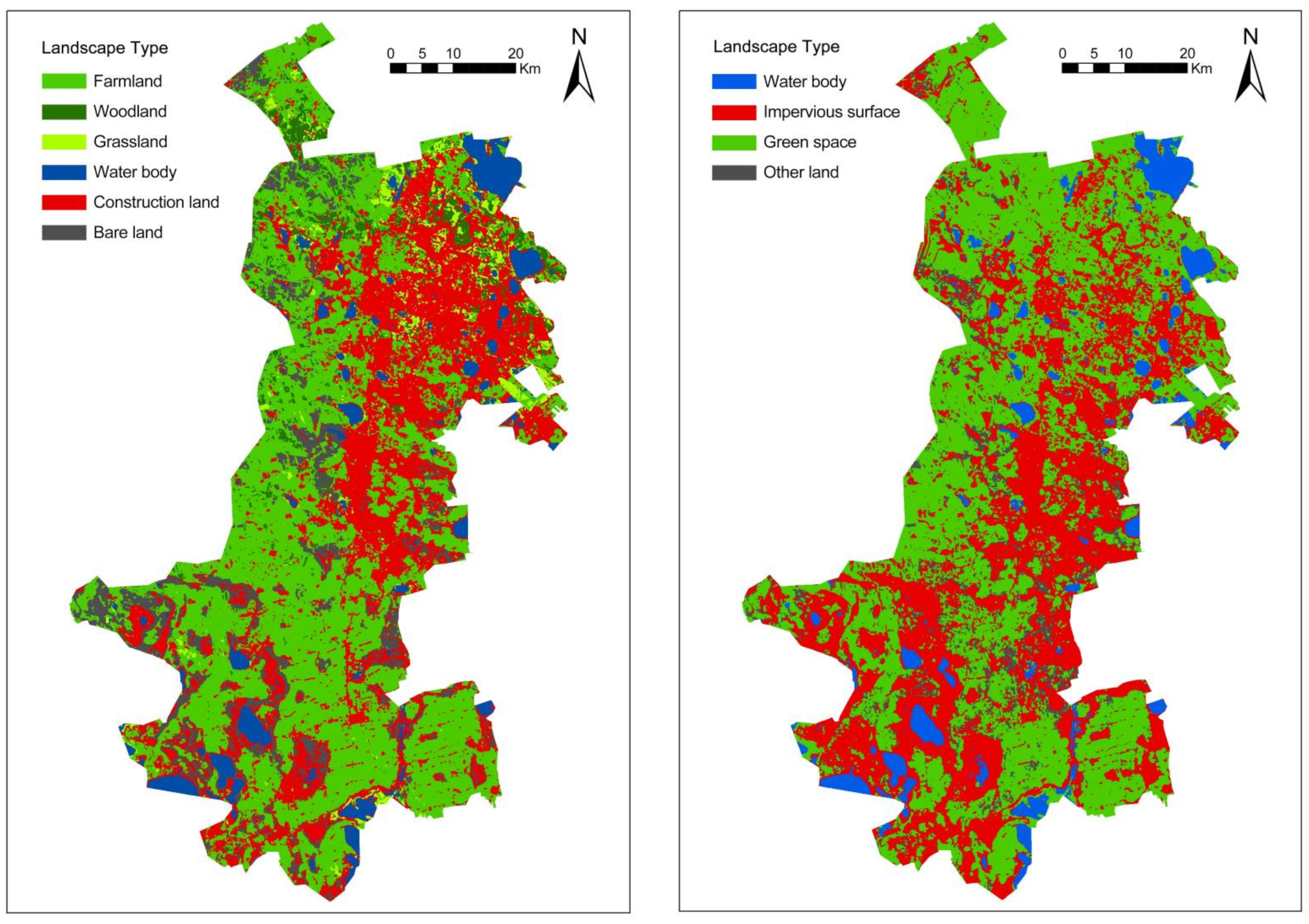
First, geometric correction was conducted on the images in the ENVI software, based on a topographic map (http://sgic.geodata.gov.cn/ (accessed on 5 June 2022)), followed by atmospheric correction for each image, using the fast line-of-sight atmospheric analysis of the spectral hypercubes (FLAASH) module, in order to eliminate atmosphere effects. Second, for the supervised classification method, the band combination was arranged according to bands 6, 5, and 4, in order to make the ground characteristics of the image clearly identifiable. Before classification, we carried out extensive field surveys in the study area, mainly by comparing the actual ground feature and remote sensing image texture at the location point, in order to determine the landscape type and training samples in the study area. Combined with the site survey results, the training and testing samples of landscape were delimited, and the resolution between samples was greater than 1.85. Then, supervised classification of the image was performed by the MLC (maximum likelihood classifier) [66]. For the spectral index-based method, the modified normalized difference water index (MNDWI) (Equation (1)), the visible red and NIR-based built-up index (VrNIR-BI) (Equation (2)), and the normalized differential vegetation index (NDVI) (Equation (3)) were adopted to extract impervious surfaces, green spaces, and water bodies, respectively [67,68,69,70]; see Table 1. Finally, the LULC of the image was classified into six types—construction land, woodland, grassland, farmland, water body, and bare land—as well as four types—green space, impervious surface, water body, and other land) (Figure 3). The overall accuracy of the supervised classification was 93.68% and the Kappa coefficient was 0.91, indicating the high accuracy of the generated image (Table 2).

$$\mathrm{MNDWI}=({\rho }_{green}-{\rho }_{swir1})/({\rho }_{green}+{\rho }_{swir1})$$

(1)

$$\mathrm{VrNIR}-\mathrm{BI}=({\rho }_{red}-{\rho }_{nir})/({\rho }_{red}+{\rho }_{nir})$$

(2)

$$\mathrm{NDVI}=({\rho }_{nir}-{\rho }_{red})/({\rho }_{nir}+{\rho }_{red})$$

(3)

where ${\rho }_{green}$, ${\rho }_{red}$, ${\rho }_{nir}$, and ${\rho }_{swir1}$ denote the reflectance of the corresponding bands in the image.

Table 1. LULC classification by the spectral index-based method.

Type	Description	Threshold Setting
Water body	Including lakes, rivers, ponds, and so on.	Otsu’s optimal binary thresholding [71]
Imperious surface	Including architectures, squares, roads, and some bare land (e.g., saline/alkali land).	VrNIR-BI ≥ −0.425, not including water body.
Green space	Including all high-coverage vegetation covers, such as forest, grass, and farmland.	NDVI ≥ 0.550, not including water body and impervious surface.
Other land	All landscape excluding the above three landscape types.	NDVI < 0.550, not including water body, impervious surface and green space.

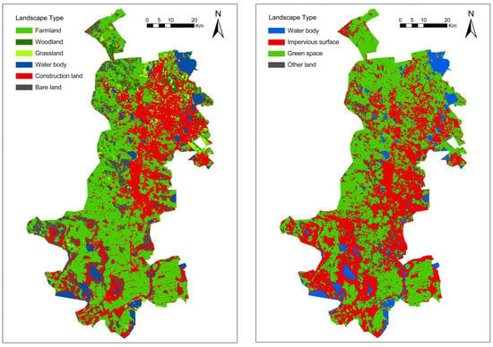
Figure 3. Landscape map classified by supervised classification method (left), and landscape map classified by spectral index-based method (right).

Table 2. The confusion matrix of supervised classification results.

	Water Body	Construction Land	Farm-Land	Bare Land	Grass-Land	Wood-Land	Total
Water body	9383	0	1		0	0	9384
Construction land	117	3767	165	463	0	0	4512
Farmland	0	54	10,589	63	37	33	10,776
Bare land	0	0	0	2535	0	0	2535
Grassland	0	2	348	0	827	0	1177
Woodland	0	9	558	0	0	315	882
Total	9500	3832	11,661	3061	864	348	29,266

2.3. Calculation of RSEI

In this paper, the RSEI is a function based on the pressure–state–response (PSR) framework, which is composed of four remote sensing indicators: Normalized differential vegetation index (NDVI), normalized differential build-up and bare soil index (NDBSI), land surface moisture (LSM), and land surface temperature (LST), reflecting the greenness, dryness, wetness, and heat of the regional environment, respectively [72,73,74]. In the PSR framework, NDBSI represents the strength of pressure on the environment generated from human disturbances, NDVI is adopted to describe the state of the environment, and LSM and LST are temperature and humidity indices indicating the response of the local climate to environmental changes. The calculation of the RSEI is detailed in the following.

2.3.1. Land Surface Moisture (LSM)

Three physical components of earth’s surface (wetness, greenness, and brightness) can be generated from the Tasseled Cap transformation (or Kauth–Thomas transformation) [75], which have been extensively applied to monitor the ecological environment [18,76]. Here, the land surface moisture parameter is represented by the wetness component, according to the following formula:

$$\mathrm{LSM}=0.1511{\rho }_{blue}+0.1972{\rho }_{green}+0.3283{\rho }_{red}+0.3407{\rho }_{nir}-0.7117{\rho }_{swir1}-0.4559{\rho }_{swir2}$$

(4)

where ${\rho }_{blue}$, ${\rho }_{green}$, ${\rho }_{red}$, ${\rho }_{nir}$, ${\rho }_{swir1}$, and ${\rho }_{swir2}$ denote the reflectance of the corresponding bands in the image.

2.3.2. Normalized Differential Vegetation Index (NDVI)

The NDVI has been extensively applied to assess vegetation growth and coverage status [74], and is expressed in Equation (3).

2.3.3. Normalized Differential Build-Up and Bare Soil Index (NDBSI)

In the previously interpreted landscape image (Figure 3), there was a large amount of construction land and bare (or thinly vegetated) land. Therefore, an index based on a combination of the build-up index (IBI) and a soil index (SI) can represent the dryness in the regional environment [18,77]. The specific formula is as follows:

$$\mathrm{NDBSI}=(\mathrm{IBI}+\mathrm{SI})/2$$

(5)

$$\mathrm{IBI}=\frac{\left\{2{\rho }_{swir1}/({\rho }_{swir1}+{\rho }_{nir})-\left[{\rho }_{nir}/({\rho }_{nir}+{\rho }_{red})+{\rho }_{green}/({\rho }_{green}+{\rho }_{swir1})\right]\right\}}{\left\{2{\rho }_{swir1}/({\rho }_{swir1}+{\rho }_{nir})+\left[{\rho }_{nir}/({\rho }_{nir}+{\rho }_{red})+{\rho }_{green}/({\rho }_{green}+{\rho }_{swir1})\right]\right\}}$$

(6)

$$\mathrm{SI}=\left[({\rho }_{swir1}+{\rho }_{red})-({\rho }_{nir}+{\rho }_{blue})\right]/\left[({\rho }_{swir1}+{\rho }_{red})+({\rho }_{nir}+{\rho }_{blue})\right]$$

(7)

where ${\rho }_{blue}$, ${\rho }_{green}$, ${\rho }_{red}$, ${\rho }_{nir}$, and ${\rho }_{swir1}$ denote the reflectance of the corresponding bands in the image.

2.3.4. Land Surface Temperature (LST)

In this study, a common method—the radiative transfer equation (RTE)—was employed to calculate the land surface temperature, as follows [27,70,78]:

$$L_{\lambda }=\tau \cdot ⎣\epsilon B(T_S)+(1-\epsilon )L\downarrow ⎦+L\uparrow$$

(8)

$$\epsilon =0.004\cdot P_V+0.986$$

(9)

$$P_V=\left\{\begin{array}{l}0,\mathrm{NDVI}<0.05\\ \left[\mathrm{NDVI}-{\mathrm{NDVI}}_{\mathrm{S}}\right]/\left[{\mathrm{NDVI}}_{\mathrm{V}}-{\mathrm{NDVI}}_{\mathrm{S}}\right] ,0.05\le \mathrm{NDVI}\le 0.7\\ 1,\mathrm{NDVI}>0.7\end{array}\right.$$

(10)

where L_λ is the at-satellite spectral radiance value; ε is the land surface emissivity of band 10 of TIRS (thermal infrared sensor); τ is the transmittance of the atmosphere of band 10 of TIRS (thermal infrared sensor); T_S is the land surface temperature; B(T_S) is the thermal radiation brightness of a black-body at T_S; and L↑ and L↓ are the upward and downward radiation light intensity of the atmosphere, respectively. Among them, τ, L↑, and L↓ can be obtained from the NASA official website (http://atmcorr.gsfc.nasa.gov/ (accessed on 21 June 2022)). Furthermore, P_V is the proportion of vegetation; NDVI_S is the vegetation index value in bare land (usually defined as 0.05) and, similarly, NDVI_V is the vegetation index value in pure vegetation land (usually defined as 0.7).

Through Equation (8), the formula for B(T_S) can be obtained as follows:

$$B\left(T_S\right)=⎣L_{\lambda }-L\uparrow -\tau \left(1-\epsilon \right)L\downarrow ⎦/\tau \epsilon$$

(11)

After obtaining B(T_S), T_S can be calculated by using the Planck formula, as follows:

$$T_S={\mathrm{K}}_2/\ln \left[{\mathrm{K}}_1/B\left(T_S\right)+1\right]$$

(12)

where K₁ and K₂ are the calibration coefficients of thermal sensor band. For TIRS, K₁ = 774.89 W/(m²·sr·μm) and K₂ = 1321.08 K.

2.3.5. RSEI Construction

Principal component analysis (PCA), as a multivariate statistical method, was adopted to integrate the above four indices. This method is a dimension reduction technique that can eliminate the effects of co-linearity among four indicators [27,74]. Significantly, according to the contribution of each factor to the principal components, the weight of all factors is automatically divided [18].

As the dimensions of the four indicators calculated above are not uniform, if each index is not normalized before conducting PCA, the weights of them will be unbalanced. Therefore, the following method was adopted to normalize the four indices to between 0 and 1 [20,32]:

$$N{I}_{\mathrm{i}}=\left(I_i-I_{\min }\right)/\left(I_{\max }-I_{\min }\right)$$

(13)

where NI_i is the normalized value of indicator i; I_i is the original value of indicator i; and I_min and I_max are the minimum and maximum values of indicator i, respectively.

After normalizing the four indicators, the RSEI was obtained using the calculation of PC1 (the first principal component) and calculated in the ENVI software, with a higher value representing better eco-environmental quality and a lower value representing poorer eco-environmental quality.

2.4. Landscape Pattern Analysis

It is of great significance to select the optimal landscape metrics when analyzing the landscape pattern. Landscape patterns can be differentiated according to the connection between components and configurations [79,80,81,82]. Based on previous studies, we defined some principles for the selection of landscape metrics: (1) The landscape metrics should represent and define the dimensions of the features of spatial patterns; (2) the landscape metrics should be easily calculated and not be complex or redundant; and (3) the landscape metrics should be those which have been previously adopted in relevant research [82,83].

Finally, according to the characteristics, effectiveness, diversity, and universality of landscape metrics in the study area, five landscape metrics were adopted: Mean Patch Size (MPS), Percentage of Landscape (PLAND), Aggregation Index (AI), Patch Density (PD), and Landscape Shape Index (LSI). The concepts and formulas for these landscape pattern metrics are presented in Table 3.

Table 3. Detailed descriptions of the selected landscape pattern metrics.

Metric (Class-Level)	Description
Mean Patch Size (MPS)	The MPS is a metric of patch area or size, which is the quotient of the patch area of a landscape type divided by the patch number in the sample unit. $\mathrm{MPS}\left(\mathrm{ha}\right)=100\times A_i/n$
Proportion of Landscape (PLAND)	The density of a landscape type in the sample unit. $\mathrm{PLAND} (\%)=100\times A_i/A$
Aggregation Index (AI)	The AI is the number of relevant patch types with similar adjacency, divided by the maximal possible number of relevant patch types with similar adjacency (0% ≤ AI ≤ 100%). The larger the value, the more aggregated the landscape. $\mathrm{AI} (\%)=100\times g_i/(\max \to g_i)$
Patch Density (PD)	Number of a landscape type patches per square kilometer in the sample unit. $\mathrm{PD}(n{/\mathrm{km}}^2)=n/A$
Landscape Shape Index (LSI)	The LSI is one of the most straightforward measures of shape complexity. LSI ≥ 1, and the closer it is to 1, the closer the shape of a patch is to a square. $\mathrm{LSI} =0.25\times P_i/\sqrt{A_i^{}}$

Remarks: A_i (km²) is the total patch area of the landscape type i; A (km²) is the total area of the sample unit; n is the patch number of the landscape type i; P_i (km) is the total patch perimeter of the landscape type i; g_i is the number of similar adjacency patches of landscape type i; max→g_i is the maximum number of similar adjacency patches between pixels of landscape type i, based on the single-count method.

2.5. Calculation of Hemeroby

Hemeroby has been extensively applied to assess the intensity of human disturbance on the environment, which is an index based on the area weight of different landscape types in each sample unit [7,49,50,51]. It is calculated as follows:

$$HI={\displaystyle \sum _{i=1}^{\mathrm{n}}\left(\frac{S_i}{S}\right)}\cdot C_i$$

(14)

where HI is the hemeroby index of the sample unit; i is the landscape type and n is the number of the landscape types; S_i is the area of landscape type i in the statistical unit and S is the area of the statistical unit; and C_i is the coefficient of human disturbance intensity of landscape type i, according to existing reports and the Expert Assessment Method. The value of C_i ranges from 0.0 to 10.0 (Table 4).

Table 4. The coefficients of human disturbance intensity for different landscape types.

	Farmland	Water Bodies	Grassland	Woodland	Construction Land	Bare Land
Human disturbance coefficient	8.7	2.9	3.6	4.7	9.5	2.5

2.6. Statistical and Analytical Methods

In this paper, the Pearson correlation coefficient and multiple linear regression model were adopted to explore the effects of human disturbance and different landscape patterns on the ecological environment, and geographically weighted regression (GWR) was adopted to analyze the spatial differences of these effects.

3. Results

3.1. The Status of Eco-Environmental Quality

Based on the RSEI calculation method detailed in Section 2.3, PC1–4 of the four remote sensing indices were extracted (Table 5). As a great number of water bodies are distributed in the study area, in order to avoid them affecting the load distribution of PCA, water bodies were masked when extracting the PCs. It can be seen that PC1 contributed the most among the four principal components, accounting for more than 80%. Moreover, compared with the other principal components, PC1 had a relatively higher correlation with the four remote sensing indices, including a positive correlation with NDVI and LSM, and a negative correlation with LST and NDBSI, consistent with the natural ecological truth [19]. In general, PC1 integrated the characteristics of the four remote sensing indices to a greater extent, thus better reflecting the ecological status of the study area. However, compared with previous related studies, the percent eigenvalue of PC1 was different, with more up to nearly 90% and less than 50% [27,84,85]. We assumed that the differences among the results of the above studies may be due to the following reasons: (including but not limited to) the geographic location of the study area, the type of satellite data used, acquisition time and season, and landscape type and topography. Therefore, these factors need to be taken into account when interpreting and comparing the results from different regions or scales.

Table 5. PCA results for the four remote sensing indicators.

		PC1	PC2	PC3	PC4
Correlation	LSM	0.7855	0.1170	0.5934	0.1311
	NDVI	0.6927	0.7186	−0.0606	0.0134
	NDBSI	−0.8140	−0.3943	−0.3362	0.2625
	LST	−0.9387	0.3432	0.0330	−0.0003
Contribution	Eigenvalue	0.0211	0.0042	0.0003	0.0001
	Percentage of eigenvalue (%)	82.10%	16.34%	1.17%	0.39%

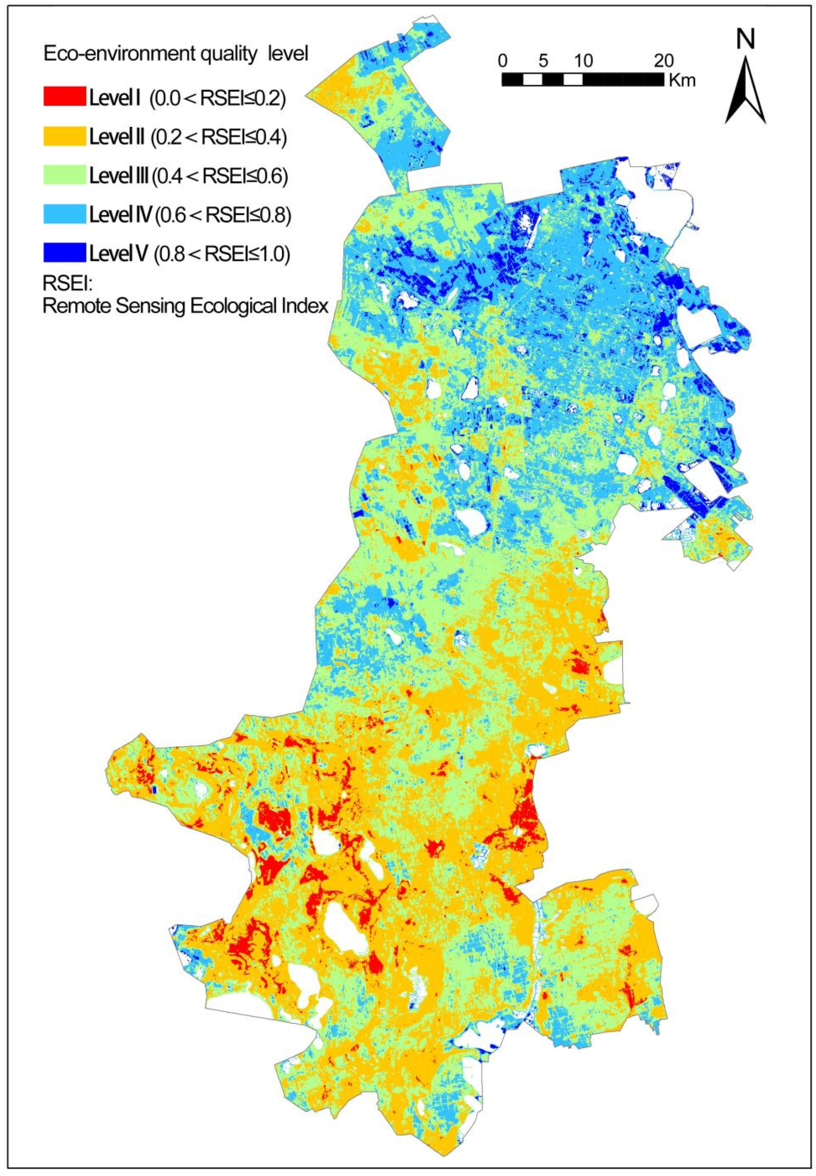
In this paper, the eco-environmental quality of the study area was divided into five levels (see Figure 4) based on the RSEI values, each with an interval of 0.2; namely, level I (poor), level II (fair), level III (moderate), level IV (good), and level V (excellent). It can be observed that the distribution of the RSEI in the study area presented significant spatial differences, showing a pattern of lower in the south and higher in the north.

Figure 4. The spatial distribution of eco-environment quality level in the study area.

Table 6 presents the areas and percentages of the RSEI at various levels. The areas of Level I–III RSEI accounted for more than 70%, while the other two levels only accounted for 27.5%. In addition, the mean RSEI value of the study area was 0.4866. These statistical results provide evidence that the eco-environmental quality of the study area was relatively moderate.

Table 6. Areas and proportions of the five eco-environmental quality levels in the study area.

Eco-Environmental Quality Level	Area (km2)	Proportion (%)
I (0.0 < RSEI ≤ 0.2)	138.05	2.92
II (0.2 < RSEI ≤ 0.4)	1498.99	31.70
III (0.4 < RSEI ≤ 0.6)	1791.24	37.88
IV (0.6 < RSEI ≤ 0.8)	1146.49	24.24
V (0.8 < RSEI ≤ 1.0)	154.08	3.26

3.2. The Status of Hemeroby and Its Correlation with RSEI

In order to explore the differences in the intensity of human interference, we classified the hemeroby into 10 levels by equal interval classification according to the value range of the hemeroby (Table 7). Furthermore, considering that forest land, grassland, water bodies, and bare land are generally weakly disturbed, while farmland and construction land are strongly disturbed, the 10 hemeroby levels were further divided into 3 hemeroby levels, based on the landscape types and hemeroby coefficients [7,54,86]. The main purpose of this classification method was to explore the relationship between human disturbance and eco-environmental quality.

Table 7. The hemeroby classification.

Hemeroby Level	Low-Level (I–VI)						Mid-Level (VII–VIII)		High-Level (IX–X)
	I	II	III	IV	V	VI	VII	VIII	IX	X
Hemeroby range	0.0–1.0	1.0–2.0	2.0–3.0	3.0–4.0	4.0–5.0	5.0–6.0	6.0–7.0	7.0–8.0	8.0–9.0	9.0–10.00

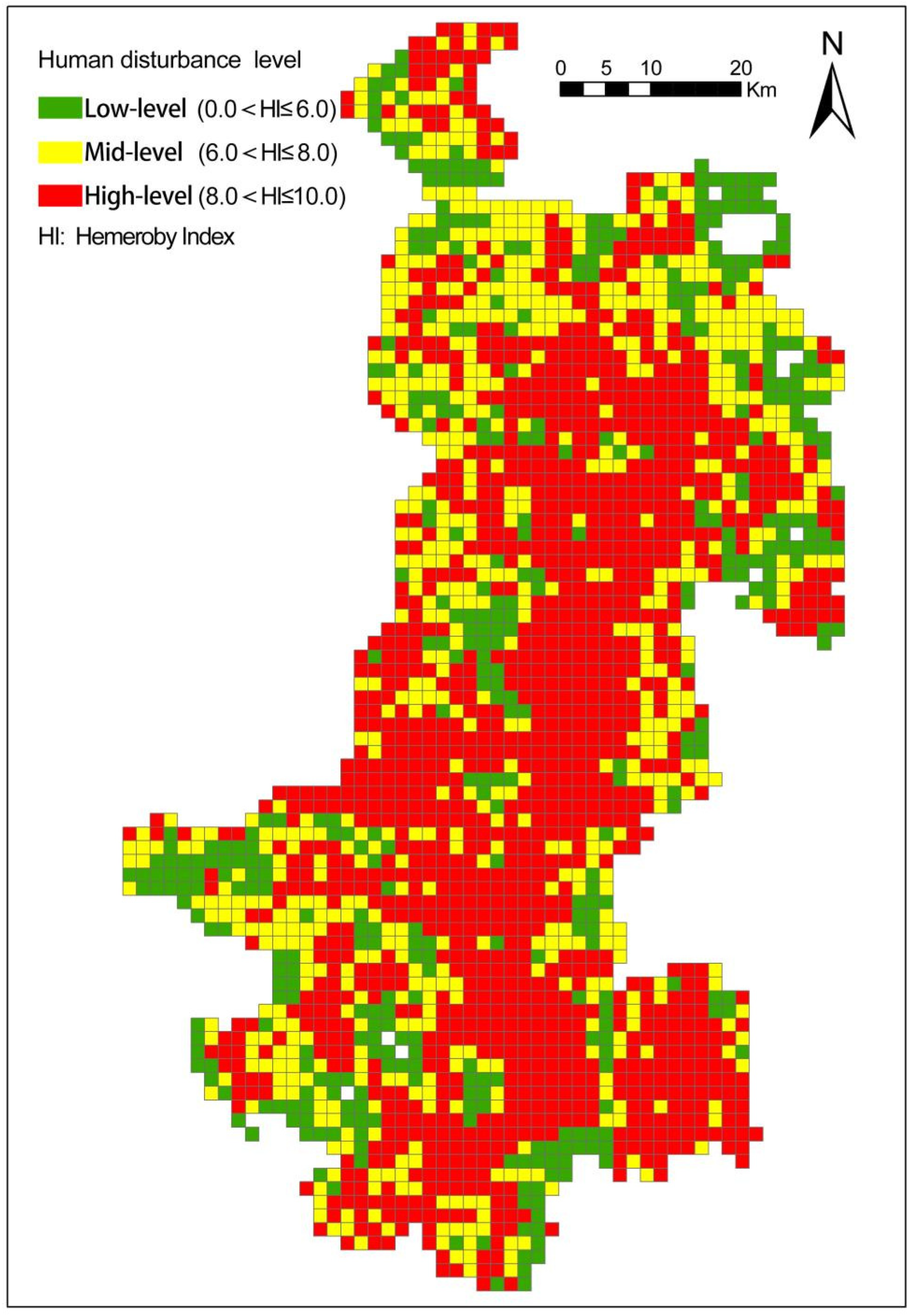
Based on Equation (14) and Table 7, the human disturbance distribution of the study area was obtained, as shown in Figure 5. As the water bodies were masked when calculating the RSEI, the grids containing only water bodies were not included in the following analysis. It can be seen that areas with high-level hemeroby were concentrated and continuous while, to the contrary, areas with low-level hemeroby were fragmented and mostly distributed on the edge of the city.

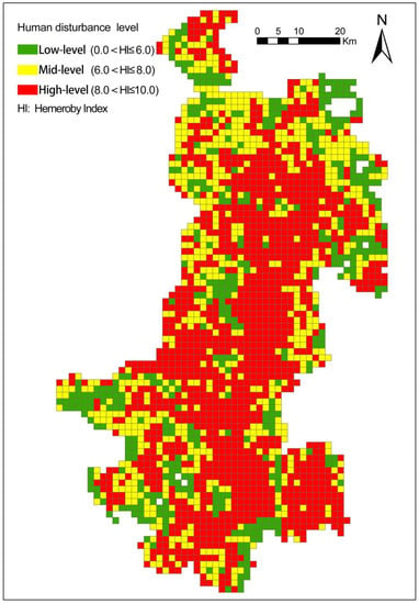
Figure 5. The spatial distribution of human disturbance level in the study area.

Table 8 provides the statistics related to the hemeroby image, indicating that the grid number of level IX hemeroby occupied the dominant position, accounting for 44.26% of all grids, followed by levels VIII and VII, which only accounted for 16.82% and 11.15%, respectively. The mean hemeroby value over the whole study area was 7.4498, indicating that human activities presented a wide range of intervention on the eco-environmental quality in the study area.

Table 8. The hemeroby statistics of the study area.

Statistical Characteristics	Grid Number	Percentage (%)	Mean Hemeroby Value
Level I	39	1.59	0.4169
Level II	25	1.02	1.6471
Level III	31	1.26	2.5490
Level IV	57	2.32	3.4879
Level V	100	4.07	4.5903
Level VI	192	7.82	5.5267
Level VII	274	11.15	6.5359
Level VIII	413	16.82	7.5469
Level IX	1087	44.26	8.5861
Level X	238	9.69	9.2458
Low-level	444	18.08	4.1789
Mid-level	687	27.97	7.1437
High-level	1325	53.95	8.7046
Whole study area	2456	100.00	7.4498

In order to analyze the effects of human disturbance on the eco-environmental quality, we calculated the mean RSEI values for all 2456 grids and analyzed the correlation with hemeroby values (Table 9). It can be observed that the mean RSEI was significantly negatively correlated with the mean hemeroby in the areas with high and low levels of hemeroby, as well as the whole study area; furthermore, this correlation was more obvious in the low-level hemeroby areas than in the high-level hemeroby areas. This result indicated that the effect of human disturbance on the eco-environmental quality was more intense in natural ecosystems, such as forests and grasslands (low-level hemeroby areas), but less intense in artificial landscapes, such as cities and farmland (high-level hemeroby areas).

Table 9. Correlations between the hemeroby values and mean RSEI values.

Region Type	Correlation	Significance
Low-level hemeroby	−0.164 **	0.001
Mid-level hemeroby	0.036	0.351
High-level hemeroby	−0.071 **	0.009
The whole study area	−0.064 **	0.002

**, Correlation is significant at the 0.01 level (two-tailed).

3.3. The Correlation of RSEI with Landscape Pattern

The previous section mainly discussed the relationship between human disturbance and eco-environmental quality using the hemeroby index, which is based on the weight of the landscape composition area. In this section, we used landscape metrics and the RSEI to study the correlation of the landscape spatial pattern with eco-environment quality.

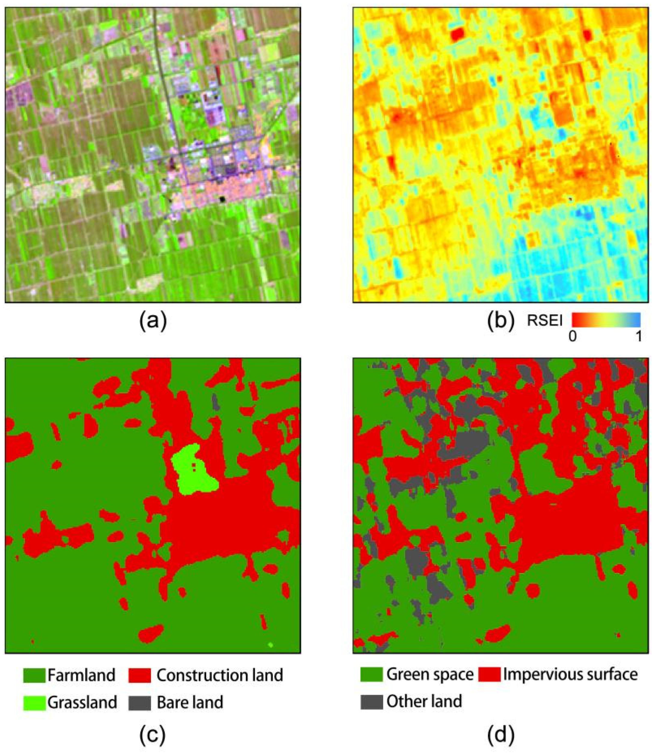
In Figure 6, the differences between the two different classification methods are represented. For example, in terms of the farmland, due to the different growth conditions, the corresponding RSEI is quite different, and this situation also occurs for woodland and grassland. If we continue to adopt the supervised classification method, the research results may be biased, which may also explain why the hemeroby was significantly correlated with the RSEI, but the correlation was not high. In contrast, the spectral index-based method can appropriately avoid this problem, as it extracts green space according to the differences in spectral reflectance, and eliminates some green spaces that are not growing well. Therefore, the image obtained with the spectral index-based method was used to explore the relationship between the landscape pattern and ecological quality.

Figure 6. Comparison of RSEI values of two classification methods in a region: (a) the original remote sensing image of a region; (b) the RSEI value of this region; (c) the landscape map of this region by supervised classification method; (d) the landscape map of this region by spectral index-based method.

Over the whole study area, compared with impervious surface and other land, green space had the largest proportion, with its patches being the largest, most regular and aggregated (see Table 10). Figure 7 presents the proportion of green space, impervious surface, and other land areas and their corresponding mean RSEI values.

Table 10. Landscape metrics at class level for the study area.

Landscape Type	PLAND	PD	LSI	MPS	AI
Green space	48.365	0.529	61.310	91.497	96.498
Impervious surface	38.987	0.625	64.479	62.339	95.894
Other land	6.313	1.481	100.887	4.262	83.920

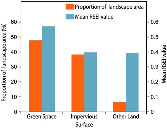
Figure 7. Proportion and mean RSEI value of each landscape type.

Table 11 presents the correlations between the spatial pattern of the three landscape types and the RSEI value. It can be seen that the PLAND of the three landscape types had the strongest correlation with the corresponding RSEI value, compared with other landscape metrics, indicating that the proportion of landscape types plays a dominant role in the impact of the RSEI. In addition to PD, the correlation between the other landscape metrics of impervious surface and the RSEI was significantly stronger than that of green space, and the correlation coefficients were opposite. This result indicates that the landscape patterns of green space and impervious surface have the opposite effect on the urban eco-environmental quality, where the effect of the former is stronger. Equations (15) and (16) present the results of the multiple linear regression taking the RSEI of green space and impervious surface as the dependent variables and the landscape metrics as the explanatory variables. The difference in the R² values can help to explain the result described above.

$${\mathrm{RSEI}}_{\mathrm{green} \mathrm{space}}=0.283+0.227\mathrm{PLAND}-0.031\mathrm{PD}+0.062\mathrm{LSI}+0.016\mathrm{MPS}+0{.089\mathrm{AI} (\mathrm{R}}^2=0.277)$$

(15)

$${\mathrm{RSEI}}_{\mathrm{impervious} \mathrm{surface}}=0.736-0.215\mathrm{PLAND}-0.171\mathrm{PD}+0.108\mathrm{LSI}-0.053\mathrm{MPS}-0{.174\mathrm{AI} (\mathrm{R}}^2=0.356)$$

(16)

Table 11. The correlation coefficients between the RSEI and landscape metrics.

Landscape Type	PLAND	PD	LSI	MPS	AI
Green space	0.538 **	−0.278 **	−0.202 **	0.510 **	0.430 **
Impervious surface	−0.577 **	0.256 **	0.271 **	−0.556 **	−0.518 **
Other land	−0.399 **	−0.222 **	−0.299 *	−0.356 **	−0.190 *

*, Correlation is significant at the 0.05 level (two-tailed); **, Correlation is significant at the 0.01 level (two-tailed).

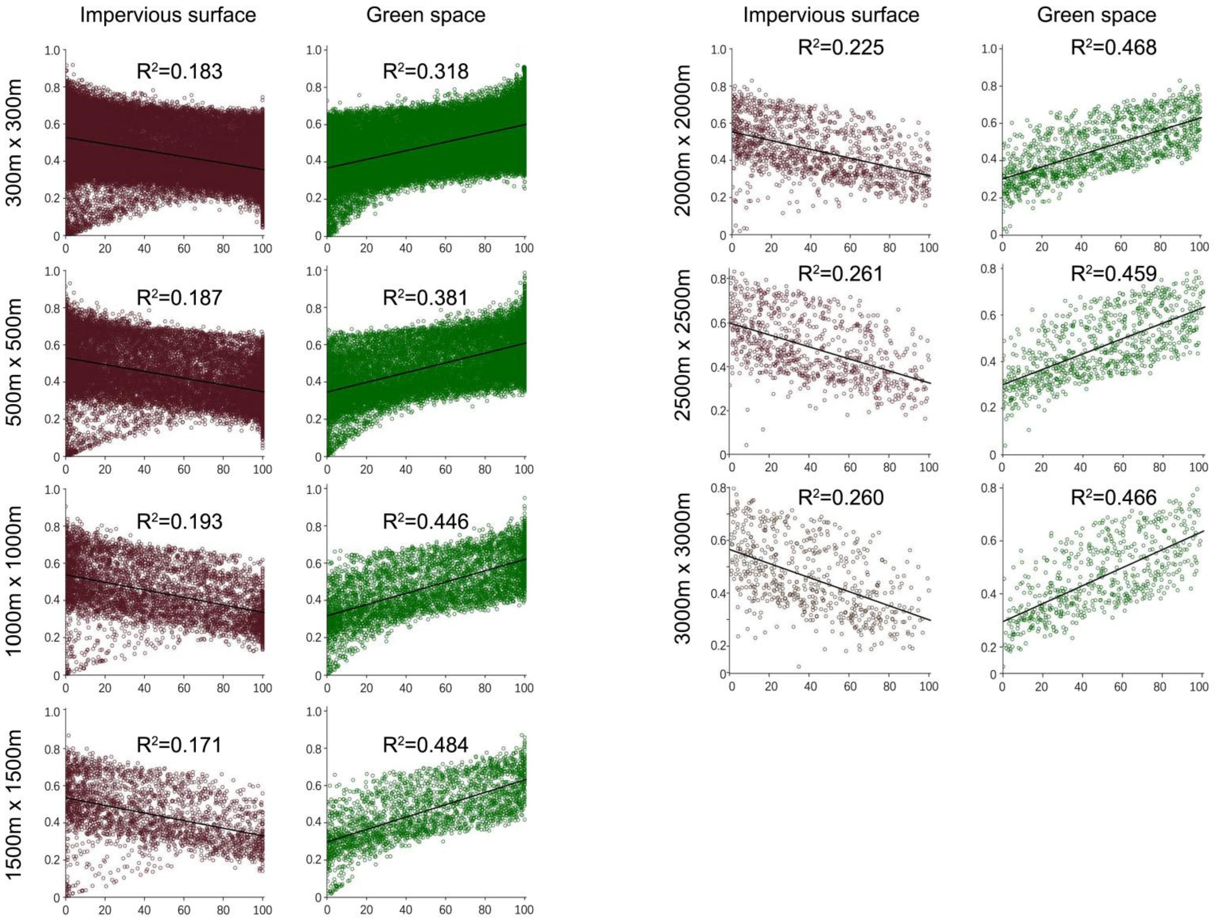
In this study, the PLAND value was selected to explore the linear relationship between the proportion of green space or impervious surface and the mean RSEI at different grid sizes (Figure 8). The results indicated that the R² values associated with green space were much higher than those with respect to impervious surface, where the R² of the green space reached a maximum in the 1.5 km × 1.5 km grid, while the R² of the impervious surface reached a maximum in the 2.5 km × 2.5 km grid, indicating that the fitting effect of green space density on eco-environmental quality was higher than that of impervious surface, and the 1.5 km × 1.5 km dimension can be considered the best characteristic area to improve the eco-environmental quality by controlling the spatial pattern of green space, while for the impervious surface it is 2.5 km × 2.5 km.

Figure 8. Linear regression results between the proportion of green space or impervious surface and the mean RSEI value at different grid sizes. The horizontal axis in each figure represents the proportion of impervious water or green space in each statistical grid (0–100%), and the vertical axis represents its corresponding mean RSEI value in each statistical grid (0.0–1.0).

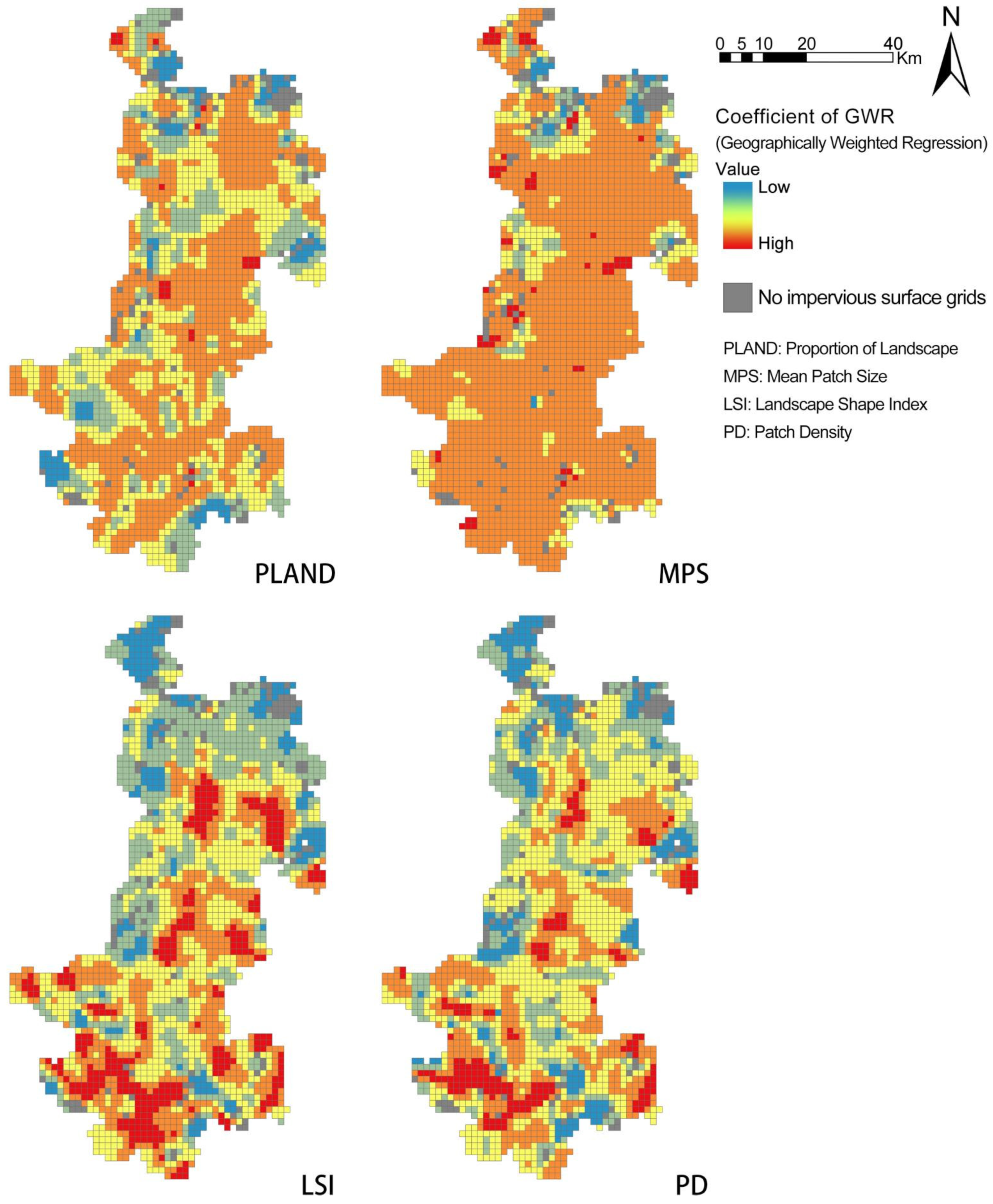
In order to further verify the relationship between an urban landscape pattern and eco-environmental quality, we adopted GWR to explore the effect of spatial differentiation of the landscape metrics on the RSEI (see Figure 9 and Figure 10). As the spatial distribution of AI (Aggregation Index) did not meet the conditions for GWR calculation, it was eliminated in subsequent analyses.

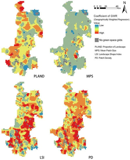
Figure 9. The geographically weighted regression analysis results of green space landscape pattern and RSEI in each statistical grid.

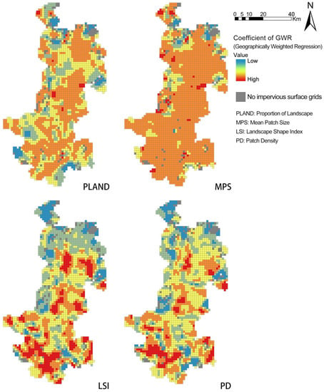
Figure 10. The geographically weighted regression analysis results of impervious surface landscape pattern and RSEI in each statistical grid.

The PLAND and MPS metrics of green space had a strong positive effect on the RSEI in urban central areas and suburban bare lands, indicating that a higher proportion and patch area of green space are helpful to improve the quality of the urban ecological environment. Only a few grids had a negative effect on the RSEI, as the green space in these grids was adjacent to a large area of water (Figure 3), resulting in a small proportion of landscape and patch area, but relatively high RSEI values. In addition, the LSI and PD metrics for green space were also positively correlated with the RSEI in the petrochemical industrial land far from the urban center, indicating that complex and scattered green space plays a positive role in improving ecological quality in these areas. Both the PLAND and MPS metrics of the impervious surface had negative effects on the RSEI, and the effects were the most obvious in the ecological lands on the edge of the city, indicating that the impervious surface poses resistance to the restoration of eco-environmental quality. The effects of the LSI and PD metrics on the RSEI in the impervious surface had similar spatial heterogeneity; that is, in the urban built-up area and suburban bare land, the fragmentation of impervious surfaces is beneficial to improving the ecological quality while, to the contrary, a large number of ecological lands are gathered in the north and edge of the city, where scattered and complex impervious surfaces may accelerate the deterioration of ecological quality.

4. Discussion

In this study, we showed that the RSEI is convenient for the evaluation of eco-environmental quality, being easy to use. It can objectively, quantitatively, and continuously classify ecological conditions in space, and can be widely used over various geographical regions. However, compared with previous related studies, the percent eigenvalue of the PC1 differed, with more up to nearly 90% and less than 50% [27,84,85]. Therefore, certain factors—such as the geographic location of the study area, the type of satellite data used, the acquisition time and season, and the landscape type and topography—need to be taken into account when interpreting and comparing the results from different regions or scales.

4.1. The Relationship between Human Disturbance and Eco-Environmental Quality

In this study, based on Equation (14) and Table 7, the human disturbance degree of the study area was calculated (Table 8), presenting a large spatial difference (Figure 5). The results showed that the area with a high level of human disturbance accounted for 53.95% and presented a centralized and continuous spatial distribution, while the area with medium and low levels of human disturbance accounted for 46.05% and presented a fragmented spatial distribution. The reason for this phenomenon may be the disorderly development of construction land and the unrestricted expansion of production land, contributing to the continuous loss of the ecological environment [7,58].

It can be seen, from the correlation between human disturbance and the eco-environmental quality of the study area, that the correlation between human disturbance and eco-environmental quality was more intense (z = −0.164, p < 0.01) in natural ecosystems, such as forests and grasslands (i.e., low-level hemeroby areas), and less intense (z = −0.071, p < 0.01) in artificial landscapes, such as cities and farmland (i.e., high-level hemeroby areas). Combined with Figure 3 and our field investigation, most areas with low RSEI values were in the southern area, where the petrochemical (i.e., high-level hemeroby areas) is distributed widely. It can be further speculated that the development of the traditional petrochemical industry has led to the pollution and deterioration of ecological land, which also verifies the previous findings [58,82,87,88].

Our findings were in line with some studies, nicely complementing them. For examples, Gutierrez et al. [89] used hemeroby to explore the relationship between human disturbance and ecological restoration, indicating that a reduction in human disturbance on forests growing in abandoned pastures resulted in a slight recovery of the forest structure and plant composition; Yang and Song [90] found that the level of human disturbance index in the high ecological vulnerability aggregation area was higher than that in the low ecological vulnerability aggregation area; and He et al. [91] analyzed the significant and negative correlation between ecological quality and human disturbance index, and pointed out that construction land and farmland were the main stress factors affecting ecological quality. However, these authors only analyzed the relationship between human disturbance and ecological quality, and did not explain the intensity of different levels of human disturbance on ecological quality.

In summary, discussing the correlation between hemeroby and the RSEI is helpful to explore the effect of human disturbance on the urban eco-environmental quality. However, for urban planners, in order to improve the eco-environmental quality, it is not enough to blindly expand ecological land and reduce the degree of human disturbance; we encourage that more attention should be paid to the protection of existing natural ecosystems, as they are more sensitive to human disturbance.

4.2. The Relationship between Urban Landscape Pattern and Eco-Environment Quality

In this study, we first calculated the landscape pattern metrics associated with green space and impervious surface (Table 10), then calculated their corresponding mean RSEI values (Figure 7) and further discussed the correlation between them (Table 11).

The results demonstrated that the proportion of green space in the study area was the largest, the degree of fragmentation was the lowest, and the shape was the most regular and concentrated. As mentioned above, the factors affecting the RSEI were diverse, such as the nature of the land-cover and the acquisition time of the satellite data [18]; therefore, we cannot define this spatial pattern of the green space as a reason for its highest RSEI value, but we can identify which landscape pattern is beneficial to improving the eco-environmental quality, by analyzing the correlation between the landscape pattern metrics and the RSEI.

According to Table 11, the landscape pattern metrics of green space and impervious surface had opposite correlation coefficients with the RSEI, and these correlations varied with different spatial locations (Figure 9 and Figure 10). Specifically, the complex and scattered green space had a positive effect on the improvement of ecological quality in the built-up area while, at the same time, the fragmentation of the impervious surface was beneficial to improving the ecological quality. The reason for this is that the diversification of patch edges might strengthen the energy conversion and flow between the green space and the ground around it, providing more shelter for the peripheral surface, leading to higher humidity and lower temperature [70,92,93]. However, the scattered and complex impervious surface will accelerate the deterioration of the ecological quality in the original complete and continuous ecological land.

Our findings were comparable to those of previous studies. For example, some studies have found that there exists a coupling relationship between the spatial pattern of impervious surface and its effect on eco-environmental quality [39,40]; however, they did not explain how it was affected. Xu et al. [18] clarified the correlation coefficients of several impervious surface pattern metrics with eco-environmental quality (RSEI) in the Xiong’an New Area, China, but the PD and LSI of the impervious surface were insignificantly correlated with the RSEI. Although the two landscape metrics were significantly correlated in our study, the correlation coefficients were relatively low. This difference may be related to the difference in research scale and the number of statistical samples; that is, we counted the landscape metrics at five RSEI levels, instead of those associated with grids. In addition, we also analyzed the different effects of spatial patterns on the RSEI with respect to impervious surface and green space. Fan et al. [94] discussed the relationships between landscape diversity, dominance, fragmentation, evenness, and eco-environmental characteristics of lake basins in Yunnan province, China, but did not classify the landscape and analyze the associated correlations. Similarly, Ji et al. [95] utilized the RSEI to understand the spatiotemporal change of the eco-environment and landscape pattern in the Jing-Jin-Ji urban agglomeration during 2001–2015; however, they also discussed the correlation between the spatial pattern at landscape-level and the RSEI. It is worth mentioning that this study considered the effect of landscape patterns on the RSEI in the temporal dimension, which will also be the focus of our future research.

In summary, the spatial pattern of the urban landscape presented a definite correlation with the eco-environmental quality. The effects of the patch proportion, area, and aggregation degree were stronger, while the effects of the patch shape and density were weaker, and these effects were heterogeneous in the spatial dimension. Therefore, it is recommended that, when optimizing the spatial arrangement of the urban landscape, urban planners should give priority to increasing the proportion of green space, disperse buildings, cluster green space, and diversify the boundary of green space in the built-up region. At the same time, in the ecological land away from the urban center, it is necessary to maintain the integrity of green space and refrain from placing fragmented building-groups.

4.3. Limitations and Future Research Directions

In this study, hemeroby and landscape metrics were adopted to analyze the correlation with the RSEI, in order to explore the effects of human disturbance and urban spatial pattern on eco-environmental quality. However, there are still some limitations that need to be further improved, as follows: (1) Interpreting the relationship between pattern and scale is a core issue in landscape ecology [96]. Although we selected the appropriate scale, according to the method proposed by O’Neill et al. [65], and verified it, there was still a strong scale effect in the interaction of multiple landscape functions, which may have affected the final results to a certain extent. Therefore, in the future, different cities can be selected for comparative research, in order to explore the effect of scale on the research results. (2) The RSEI was obtained by extracting the principal components of four remote sensing indices, according to the construction method of the PSR model. However, the contribution rate of the first principal component did not reach 100%; that is, the obtained RSEI cannot completely characterize the eco-environmental quality of the study area, which also affected the research results, to a certain extent. Therefore, improving the contribution rate of indicators or selecting more suitable indicators will be the focus of future research.

5. Conclusions

In this study, we demonstrated how to use hemeroby and the RSEI to characterize the degree of human disturbance and eco-environmental quality of a city, and established the relationship between them. The results demonstrated that the RSEI can better reflect the eco-environmental quality of the whole study area The mean RSEI value was 0.4866, which was at a relatively moderate level, presenting a spatial differentiation of low in the south and high in the north. The mean hemeroby value over the whole study area was 7.4498, indicating that human activities have had a wide range of intervention on the ecological environment. By analyzing the correlation between hemeroby and the RSEI in different levels of human disturbance areas, it was found that the effect of human disturbance on the eco-environmental quality was more intense in natural ecosystems, such as forests and grasslands (i.e., low-level hemeroby area) but less intense in artificial landscapes, such as cities and farmland (i.e., a high-level hemeroby area). Therefore, compared with reducing the degree of human disturbance in urban built-up areas, it is better to focus on protecting the existing natural ecosystems, as their ecological quality is more sensitive to human disturbances.

The spatial pattern is an important feature of the landscape. Hence, it is particularly important to explore the effect of the spatial pattern on the eco-environmental quality. In this study, we first analyzed the correlation between the spatial pattern of different landscape types and the RSEI, followed by the spatial variation of the effect of landscape patterns on the RSEI, based on the GWR model. The results indicated that the selected five landscape pattern metrics were all significantly correlated with the RSEI, and the landscape pattern metrics of green space and impervious surface had opposite effects on the urban eco-environmental quality, where the effect of the former was stronger. The results of the GWR model provided evidence for the spatial variation of the effect of the landscape pattern on the RSEI, showing that, in the urban built-up area, the complex and scattered impervious surface and green space can help to improve the ecological quality while, to the contrary, the fragmentation of impervious surface may accelerate the deterioration of the vast natural ecological lands.

Finally, the relevant methods described in this study had no regional restrictions and, so, can also be used in other locations. We hope that our findings will provide beneficial reference for urban planners and policy makers.

References

- Foley, J.N.; Ramankutty, K.A.; Brauman, E.S.; Cassidy, J.S.; Gerber, M.; Johnston, N.D.; Mueller, C.O.; Connell, D.K.; Ray, P.C.; West, C.; et al. Solutions for a cultivated planet. Nature 2011, 478, 337–342. [Google Scholar] [CrossRef] [PubMed]
- Orimoloye, I.R.; Ololade, O.O.; Mazinyo, S.P.; Kalumba, A.M.; Ekundayo, O.Y.; Busayo, E.T.; Nel, W. Spatial assessment of drought severity in Cape Town area, South Africa. Heliyon 2019, 5, e02148. [Google Scholar] [CrossRef] [PubMed]
- Mark, M.; Oshneck, M.; Tatenda, M.; Rameck, D. A GIS and remote sensing aided assessment of land use/cover changes in resettlement areas; a case of ward 32 of Mazowe district, Zimbabwe. J. Environ. Manag. 2020, 276, 111312. [Google Scholar] [CrossRef]
- Halpern, B.S.; Walbridge, S.; Selkoe, K.A.; Kappel, C.V.; Micheli, F.; Dagrosa, C.; Bruno, J.F.; Casey, K.S.; Ebert, C.; Fox, H.E.; et al. A global map of human impact on marine ecosystems. Science 2008, 319, 948–952. [Google Scholar] [CrossRef]
- Vitousek, P.M.; Mooney, H.A.; Lubchenco, J.; Melillo, J.M. Human domination of earth’s ecosystems. Science 1997, 277, 494–499. [Google Scholar] [CrossRef]
- Balter, M. Archaeology Archaeologists say the “Anthropocene” is here—But it began long ago. Science 2013, 340, 261–262. [Google Scholar] [CrossRef]
- Zhou, Y.K.; Ning, L.X.; Bai, X.L. Spatial and temporal changes of human disturbances and their effects on landscape patterns in the Jiangsu coastal zone, China. Ecol. Ind. 2018, 93, 111–122. [Google Scholar] [CrossRef]
- Foley, J.A.; DeFries, R.; Asner, G.P.; Barford, C.; Bonan, G.; Carpenter, S.R.; Snyder, P.K. Global consequences of land use. Science 2005, 309, 570–574. [Google Scholar] [CrossRef]
- Song, X.; Hansen, M.C.; Stehman, S.V.; Potapov, P.V.; Tyunkvina, A.; Vermote, E.F.; Townshend, J.R. Global land change from 1982 to 2016. Nature 2018, 560, 639–643. [Google Scholar] [CrossRef]
- Rahaman, S.; Kumar, P.; Chen, R.; Meadows, M.E.; Singh, R.B. Remote sensing assessment of the impact of land use and land cover change on the environment of Barddhaman District, West Bengal, India. Front. Environ. Sci. 2020, 8, 127. [Google Scholar] [CrossRef]
- Briassoulis, H. Factors influencing land-use and land-cover change. UNESCO Encycl. Life Support Syst. 2009, 1, 126–146. [Google Scholar]
- Mainuri, Z.G.; Owino, J.O. Linking landforms and land use to land degradation in the Middle River Njoro watershed. Int. Soil Water Conserv. Res. 2014, 2, 1–10. [Google Scholar] [CrossRef]
- Ayanlade, A.; Howard, M.T. Understanding changes in a Tropical Delta: A multimethod narrative of land use or land cover change in the Niger Delta. Ecol. Model. 2017, 364, 53–65. [Google Scholar] [CrossRef]
- Wang, C.L.; Jiang, Q.O.; Shao, Y.Q.; Sun, S.Y.; Xiao, L.; Guo, J.B. Ecological environment assessment based on land use simulation: A case study in the Heihe River Basin. Sci. Total Environ. 2019, 697, 133928. [Google Scholar] [CrossRef]
- Weng, Q.H. Thermal infrared remote sensing for urban climate and environmental studies: Methods, applications, and trends. ISPRS J. Photogramm. Remote Sens. 2009, 64, 335–344. [Google Scholar] [CrossRef]
- Zhou, D.C.; Zhao, S.Q.; Liu, S.G.; Zhang, L.X.; Zhu, C. Surface urban heat island in China’s 32 major cities: Spatial patterns and drivers. Remote Sens. Environ. 2014, 152, 51–61. [Google Scholar] [CrossRef]
- Willis, K.S. Remote sensing change detection for ecological monitoring in United States protected areas. Biol. Conserv. 2015, 182, 233–242. [Google Scholar] [CrossRef]
- Hu, X.S.; Xu, H.Q. A new remote sensing index for assessing the spatial heterogeneity in urban ecological quality: A case from Fuzhou City, China. Ecol. Indic. 2018, 89, 11–21. [Google Scholar] [CrossRef]
- Xu, H.Q.; Wang, M.Y.; Shi, T.T.; Guan, H.; Fang, C.Y.; Lin, Z.L. Prediction of ecological effects of potential population and impervious surface increases using a remote sensing based ecological index (RSEI). Ecol. Indic. 2018, 93, 730–740. [Google Scholar] [CrossRef]
- Carlson, T.N.; Arthur, S.T. The impact of land use-land cover changes due to urbanization on surface microclimate and hydrology: A satellite perspective. Glob. Planet. Chang. 2000, 25, 49–65. [Google Scholar] [CrossRef]
- Buyantuyev, A.; Wu, J. Urban heat islands and landscape heterogeneity: Linking spatiotemporal variations in surface temperatures to land-cover and socioeconomic patterns. Landsc. Ecol. 2010, 25, 17–33. [Google Scholar] [CrossRef]
- Cao, Q.; Yu, D.; Georgescu, M.; Han, Z.; Wu, J. Impacts of land use and land cover change on regional climate: A case study in the agro-pastoral transitional zone of China. Environ. Res. Lett. 2015, 10, 124025. [Google Scholar] [CrossRef]
- Cai, Y.B.; Zhang, H.; Zheng, P.; Pan, W.B. Quantifying the impact of land use/land cover changes on the urban heat island: A case study of the natural wetlands distribution area of Fuzhou City, China. Wetlands 2016, 36, 285–298. [Google Scholar] [CrossRef]
- Yin, J.; Wu, X.X.; Shen, M.G.; Zhang, X.L.; Zhu, C.H.; Xiang, H.X.; Shi, C.M.; Guo, Z.Y.; Li, C.L. Impact of urban green space spatial pattern on land surface temperature: A case study in Beijing metropolitan area, China. Landsc. Ecol. 2019, 34, 2949–2961. [Google Scholar] [CrossRef]
- Honnay, O.; Piessens, K.; Van Landuyt, W.; Hermy, M.; Gulinck, H. Satellite based land use and landscape complexity indices as predictors for regional plant species diversity. Landsc. Urban Plan. 2003, 63, 241–250. [Google Scholar] [CrossRef]
- Grecchi, R.C.; Gwyn, Q.H.; Bénié, G.B.; Formaggio, A.R.; Fahl, F.C. Land use and land cover changes in the Brazilian Cerrado: A multidisciplinary approach to assess the impacts of agricultural expansion. Appl. Geogr. 2014, 55, 300–312. [Google Scholar] [CrossRef]
- Xu, H.Q. A remote sensing urban ecological index and its application. Acta Ecol. Sin. 2013, 33, 7853–7862. [Google Scholar]
- Wen, X.L.; Lin, Z.F.; Tang, F. Remote sensing analysis of ecological change caused by construction of the new island city: Pingtan Comprehensive Experimental Zone, Fujian Province. J. Appl. Ecol. 2015, 26, 541–547. [Google Scholar] [CrossRef]
- Qureshi, S.; Alavipanah, S.K.; Konyushkova, M.; Mijani, N.; Fathololomi, S.; Firozjaei, M.K.; Homaee, M.; Hamzeh, S.; Kakroodi, A.A. A Remotely Sensed Assessment of Surface Ecological Change over the Gomishan Wetland, Iran. Remote Sens. 2020, 12, 2989. [Google Scholar] [CrossRef]
- Yue, H.; Liu, Y.; Li, Y.; Lu, Y. Eco-environmental quality assessment in China’s 35 major cities based on remote sensing ecological index. IEEE Access 2019, 7, 51295–51311. [Google Scholar] [CrossRef]
- Zheng, Z.H.; Wu, Z.F.; Chen, Y.B.; Yang, Z.W.; Marinello, F. Exploration of eco-environment and urbanization changes in coastal zones: A case study in China over the past 20 years. Ecol. Indic. 2020, 119, 106847. [Google Scholar] [CrossRef]
- Shan, W.; Jin, X.B.; Ren, J.; Wang, Y.C.; Xu, Z.G.; Fan, Y.T.; Gu, Z.M.; Hong, C.Q.; Lin, J.H.; Zhou, Y.K. Ecological environment quality assessment based on remote sensing data for land consolidation. J. Clean. Prod. 2019, 239, 118126. [Google Scholar] [CrossRef]
- Zhu, D.Y.; Chen, T.; Zhen, N.; Niu, R.Q. Monitoring the effects of open-pit mining on the eco-environment using a moving window-based remote sensing ecological index. Environ. Sci. Pollut. Res. 2020, 27, 15716–15728. [Google Scholar] [CrossRef] [PubMed]
- Ariken, M.; Zhang, F.; Liu, K.; Fang, C.L.; Kung, H.T. Coupling coordination analysis of urbanization and eco-environment in Yanqi Basin based on multi-source remote sensing data. Ecol. Indic. 2020, 114, 106331. [Google Scholar] [CrossRef]
- Gong, E.J.; Shi, F.X.; Wang, Z.H.; Hu, Q.F.; Zhang, J.; Hai, H.X. Evaluating environmental quality and its driving force in northeastern China using the remote sensing ecological index. Sustainability 2022, 14, 16304. [Google Scholar] [CrossRef]
- Yang, Z.J.; Sun, C.; Ye, J.W.; Gan, C.Y.; Li, Y.; Wang, L.Y.; Chen, Y.J. Spatio-temporal heterogeneity of ecological quality in Hangzhou greater bay area (HGBA) of china and response to land use and cover change. Remote Sens. 2022, 14, 5613. [Google Scholar] [CrossRef]
- Zhang, Y.; She, J.Y.; Long, X.R.; Zhang, M. Spatio-temporal evolution and driving factors of eco-environmental quality based on RSEI in Chang-Zhu-Tan metropolitan circle, central China. Ecol. Indic. 2022, 144, 109436. [Google Scholar] [CrossRef]
- Koellner, T.; Scholz, R.D. Assessment of land use impacts on the natural environment: Part 1: An Analytical Framework for Pure Land Occupation and Land Use Change. Int. J. Life Cycle Assess. 2007, 12, 16–23. [Google Scholar] [CrossRef]
- Wickham, J.D.; Wade, T.G.; Norton, D.J. Spatial patterns of watershed impervious cover relative to stream location. Ecol. Indic. 2014, 40, 109–116. [Google Scholar] [CrossRef]
- Beck, S.M.; McHale, M.R.; Hes, G.R. Beyond impervious: Urban land-cover pattern variation and implications for watershed management. Environ. Manag. 2016, 58, 15–30. [Google Scholar] [CrossRef]
- Wan, R.R.; Yang, G.S. Changes of land use and landscape pattern in Taihu Lake Basin. Chin. J. Appl. Ecol. 2005, 16, 475–480. [Google Scholar] [CrossRef]
- Li, H.Y.; Man, W.D.; Li, X.Y.; Ren, C.Y.; Wang, Z.M.; Li, L.; Jia, M.M.; Mao, D.H. Remote sensing investigation of anthropogenic land cover expansion in the low elevation coastal zone of Liaoning Province, China. Ocean Coast. Manag. 2017, 148, 245–259. [Google Scholar] [CrossRef]
- Sukopp, H. Der Einfluss des Menschen auf die Vegetation. Plant Ecol. 1969, 17, 360–371. [Google Scholar] [CrossRef]
- Novakovskaya, T.V.; Akulshina, N.P. Application of geobotanical indices of ecological scale to mapping of disturbed lands in the Khar’ yaginsk Oil and Gas Field. Russ. J. Ecol. 1997, 28, 224–229. [Google Scholar]
- Li, M.; Kruchi, N.; Yang, J. Hemeroby—A method to assess the naturalness of vegetation. Prog. Geogr. 2002, 21, 450–458. [Google Scholar] [CrossRef]
- Zebisch, M.; Wechsung, F.; Kenneweg, H. Landscape response functions for biodiversity-assessing the impact of land-use changes at the county level. Landsc. Urban Plan. 2004, 67, 157–172. [Google Scholar] [CrossRef]
- Fu, B.J.; Hu, C.X.; Chen, L.D.; Honnay, O.; Gulinck, H. Evaluating change in agricultural landscape pattern between 1980 and 2000 in the Loess hilly region of Ansai County, China. Agric. Ecosyst. Environ. 2006, 114, 387–396. [Google Scholar] [CrossRef]
- Chen, A.L.; Zhu, B.Q.; Chen, L.D.; Wu, Y.H.; Sun, R.H. Dynamic changes of landscape pattern and eco-disturbance degree in Shuangtai estuary wet land of Liaoning Province, China. Chin. J. Appl. Ecol. 2010, 21, 1120–1128. [Google Scholar] [CrossRef]
- Grizzetti, B.; Lanzanova, D.; Liquete, C.; Reynaud, A.; Cardoso, A.C. Assessing water ecosystem services for water resource management. Environ. Sci. Policy 2016, 61, 194–203. [Google Scholar] [CrossRef]
- Wellmann, T.; Haase, D.; Knapp, S.; Salbach, C.; Selsam, P.; Laush, A. Urban land use intensity assessment: The potential of spatio-temporal spectral traits with remote sensing. Ecol. Indic. 2018, 85, 190–203. [Google Scholar] [CrossRef]
- Tian, Y.; Liu, B.X.; Hu, Y.D.; Xu, Q.; Xu, D.W. Spatio-Temporal Land-Use Changes and the Response in Landscape Pattern to Hemeroby in a Resource-Based City. ISPRS Int. J. Geo-Inf. 2020, 9, 20. [Google Scholar] [CrossRef]
- Geri, F.; Amici, V.; Rocchini, D. Human activity impact on the heterogeneity of Mediterranean landscape. Appl. Geogr. 2010, 30, 370–379. [Google Scholar] [CrossRef]
- Sun, Y.G.; Zhao, D.Z.; Wu, T.; Wei, B.Q.; Gao, S.G.; Li, Y.; Cao, F.F. Temporal and spatial dynamic changes and landscape pattern response of Hemeroby in Dayang estuary of Liaoning Province, China. Acta Ecol. Sin. 2012, 32, 3645–3655. [Google Scholar] [CrossRef]
- Ning, J.; Liu, J.Y.; Zhao, G.S. Spatio-temporal characteristics of disturbance of land use change on major ecosystem function zones in China. Chin. Geogr. Sci. 2015, 25, 523–536. [Google Scholar] [CrossRef]
- Roth, D.; Moreno-Sanchez, R.; Torres-Rojo, J.M.; Moreno-Sanchez, F. Estimation of human induced disturbance of the environment associated with 2002, 2008 and 2013 land use/cover patterns in Mexico. Appl. Geogr. 2016, 66, 22–34. [Google Scholar] [CrossRef]
- Guo, S.Z.; Bai, H.Y.; Meng, Q.; Huang, X.Y.; Qi, G.Z. The change of landscape pattern in Qinling mountains from 1980 to 2015 and its response to human disturbance. Chin. J. Appl. Ecol. 2018, 29, 4080–4088. [Google Scholar] [CrossRef]
- Long, H.; Tang, G.; Li, X.; Heilig, G.K. Socio-economic driving forces of land-use change in Kunshan, the Yangtze River Delta economic area of China. J. Environ. Manag. 2007, 83, 351–364. [Google Scholar] [CrossRef]
- Deng, X.Z.; Huang, J.K.; Rozelle, S.; Uchida, E. Growth, population and industrialization, and urban land expansion of China. J. Urban Econ. 2008, 63, 96–115. [Google Scholar] [CrossRef]
- Salhi, A.; Benabdelouahab, S.; Bouayad, E.O.; Benabdelouahab, T.; Larifi, I.; Mousaoui, M.E.; Acharrat, N.; Himi, M.; Ponsati, A.C. Impacts and social implications of land-use environment conflicts in a typical Mediterranean watershed. Sci. Total Environ. 2020, 764, 142853. [Google Scholar] [CrossRef]
- Walz, U.; Stein, C. Indicators of hemeroby for the monitoring of landscapes in Germany. J. Nat. Conserv. 2014, 22, 279–289. [Google Scholar] [CrossRef]
- Beynen, P.V.; Townsend, K. A disturbance index for Karst environments. Environ. Manag. 2005, 36, 101–116. [Google Scholar] [CrossRef]
- Zhao, D.D.; Liu, J.P. Heterogeneity of wetland landscapes and their relationships with anthropogenic disturbances and precipitation in a semiarid region of China. Environ. Monit. Assess. 2022, 194, 786. [Google Scholar] [CrossRef] [PubMed]
- Jasinaviciute, A.; Veteikis, D. Assessing landscape instability through land-cover change based on the hemeroby index (Lithuanian example). Land 2022, 11, 1056. [Google Scholar] [CrossRef]
- Liu, H.; Zhao, Z.; Zhang, G.S.; Su, J. Thoughts and Explorations on the Transformation of Petroleum Resource-based Cities: A Case Study of Daqing City (Daqing Oilfield). Pet. Geol. Oilfield Dev. Daqing 2019, 38, 1–5. [Google Scholar] [CrossRef]
- O’Neill, R.V.; Hunsaker, C.T.; Timmins, S.P.; Jackson, B.L.; Jones, K.B.; Riitters, K.H.; Wickham, J.D. Scale problems in reporting landscape pattern at the regional scale. Landsc. Ecol. 1996, 11, 169–180. [Google Scholar] [CrossRef]
- Aghsaei, H.; Dinan, N.M.; Moridi, A.; Asadolahi, Z.; Delavar, M.; Fohrer, N.; Wagner, P.D. Effects of dynamic land use/land cover change on water resources and sediment yield in the Anzali wetland catchment, Gilan, Iran. Sci. Total Environ. 2020, 712, 136449. [Google Scholar] [CrossRef] [PubMed]
- Rouse, J.W.; Haas, R.H.; Schell, J.A.; Deering, D.W. Monitoring Vegetation Systems in the Great Plains with ERTS. In Proceedings of the 3rd Earth Resources Technology Satellite-1 Symposium, Washington, DC, USA, 10–14 December 1973; NASA: Washington, DC, USA, 1974; pp. 309–317. [Google Scholar]
- Xu, H. Modification of normalized difference water index (NDWI) to enhance open water features in remotely sensed imagery. Int. J. Remote Sens. 2006, 27, 3025–3033. [Google Scholar] [CrossRef]
- Estoque, R.C.; Murayama, Y. Classification and change detection of built-up lands from Landsat-7 ETM+ and Landsat-8 OLI/TIRS imageries: A comparative assessment of various spectral indices. Ecol. Indic. 2015, 56, 205–217. [Google Scholar] [CrossRef]
- Estoque, R.C.; Murayama, Y.; Myint, S.W. Effects of landscape composition and pattern on land surface temperature: An urban heat island study in the megacities of Southeast Asia. Sci. Total Environ. 2017, 577, 349–359. [Google Scholar] [CrossRef]
- Otsu, N. A threshold selection method from gray-level histograms. IEEE Trans. Syst. Man Cybern. 1979, 9, 62–66. [Google Scholar] [CrossRef]
- Lin, T.; Ge, R.B.; Huang, J.; Zhao, Q.J.; Lin, J.Y.; Huang, N.; Zhang, G.Q.; Li, X.H.; Ye, H.; Yin, K. A quantitative method to assess the ecological indicator system’s effectiveness: A case study of the ecological province construction indicators of China. Ecol. Indic. 2016, 62, 95–100. [Google Scholar] [CrossRef]
- Niemi, G.J.; McDonald, M.E. Application of ecological indicators. Annu. Rev. Ecol. Evol. Syst. 2004, 35, 89–111. [Google Scholar] [CrossRef]
- Seddon, A.W.R.; Macias-Fauria, M.; Long, P.R.; Benz, D.; Willis, K.J. Sensitivity of global terrestrial ecosystems to climate variability. Nature 2016, 531, 229–232. [Google Scholar] [CrossRef] [PubMed]
- Zawadzki, J.; Przeździecki, K.; Miatkowski, Z. Determining the area of influence of depression cone in the vicinity of lignite mine by means of triangle method and Landsat TM/ETM+ satellite images. J. Environ. Manag. 2016, 166, 605–614. [Google Scholar] [CrossRef]
- Goward, S.N.; Xue, Y.K.; Czajkowski, K.P. Evaluating land surface moisture conditions from the remotely sensed temperature/vegetation index measurements: An exploration with the simplified simple biosphere model. Remote Sens. Environ. 2002, 79, 225–242. [Google Scholar] [CrossRef]
- Essa, W.; Verbeiren, B.; van der Kwast, J.; Van de Voorde, T.; Batelaan, O. Evaluation of the DisTrad thermal sharpening methodology for urban areas. Int. J. Appl. Earth Obs. Geoinf. 2012, 19, 163–172. [Google Scholar] [CrossRef]
- Chander, G.; Markham, B.L.; Helder, D.L. Summary of current radiometric calibration coefficients for Landsat MSS, TM, ETM+, and EO-1 ALI sensors. Remote Sens. Environ. 2009, 113, 893–903. [Google Scholar] [CrossRef]
- Gustafson, E.J. Quantifying Landscape Spatial Pattern: What is the state of the art? Ecosystems 1998, 1, 143–156. [Google Scholar] [CrossRef]
- Slager, C.T.J.; Vries, B.D. Landscape generator: Method to generate landscape configurations for spatial plan-making. Comput. Environ. Urban Syst. 2013, 39, 1–11. [Google Scholar] [CrossRef]
- Kwok, A.; Cheung, L.; Brierley, G.; Sullivan, D.O. Landscape structure and dynamics on the Qinghai-Tibetan Plateau. Ecol. Model. 2016, 339, 7–22. [Google Scholar] [CrossRef]
- Hashem, D.; Parviz, A.; Mahdis, M. Land use change, urbanization, and change in landscape pattern in a metropolitan area. Sci. Total Environ. 2019, 655, 707–719. [Google Scholar] [CrossRef]
- Su, S.; Wang, Y.; Luo, F.; Mai, G.; Pu, J. Peri-urban vegetated landscape pattern changes in relation to socioeconomic development. Ecol. Indic. 2014, 46, 477–486. [Google Scholar] [CrossRef]
- Yang, X.Y.; Meng, F.; Fu, P.J.; Zhang, Y.X.; Liu, Y.H. Spatiotemporal change and driving factors of the Eco-Environment quality in the Yangtze River Basin from 2001 to 2019. Ecol. Indic. 2021, 131, 108214. [Google Scholar] [CrossRef]
- Airiken, M.; Zhang, F.; Chan, N.W.; Kung, H.T. Assessment of spatial and temporal ecological environment quality under land use change of urban agglomeration in the North Slope of Tianshan, China. Environ. Sci. Pollut. Res. 2021, 29, 12282–12299. [Google Scholar] [CrossRef] [PubMed]
- Raine, R.M. Current land use and changes in land use in the coastal zone of Chanthaburi Province, Thailand. Biol. Conserv. 1994, 67, 201–204. [Google Scholar] [CrossRef]
- Baus, P.; Kovac, U.; Paudisova, E.; Kohutkova, I.; Kornornik, J. Identification of interconnections between landscape pattern and urban dynamics-Case study Bratislava, Slovakia. Ecol. Indic. 2014, 42, 104–111. [Google Scholar] [CrossRef]
- Peng, J.H.; Zhao, Z.Q.; Yin, G.J. Evaluation of urban land resource value based on sustainable environment space governance. Alex. Eng. J. 2022, 61, 5585–5593. [Google Scholar] [CrossRef]
- Gutierrez, N.; Gartner, S.; Lopez, J.Y.; Pacheco, C.E.; Reif, A. The recovery of the lower montane cloud forest in the Mucujun watershed, Merida, Venezuela. Reg. Environ. Chang. 2013, 13, 1069–1085. [Google Scholar] [CrossRef]
- Yang, Y.J.; Song, G. Human disturbance changes based on spatiotemporal heterogeneity of regional ecological vulnerability: A case study of Qiqihaer city, northwestern Songnen Plain, China. J. Clean. Prod. 2021, 291, 125262. [Google Scholar] [CrossRef]
- He, B.; Chang, J.X.; Guo, A.J.; Wang, Y.M.; Wang, Y.; Li, Z.H. Assessment of river basin habitat quality and its relationship with disturbance factors: A case study of the Tarim River Basin in Northwest China. J. Arid Land 2022, 14, 167–185. [Google Scholar] [CrossRef]
- Zhou, W.; Huang, G.; Cadenasso, M.L. Does spatial configuration matter? Understanding the effects of land cover pattern on land surface temperature in urban landscapes. Landsc. Urban Plan. 2011, 102, 54–63. [Google Scholar] [CrossRef]
- Li, X.; Zhou, W.; Ouyang, Z.; Xu, W.; Zheng, H. Spatial pattern of greenspace affects land surface temperature: Evidence from the heavily urbanized Beijing metropolitan area, China. Landsc. Ecol. 2012, 27, 887–898. [Google Scholar] [CrossRef]
- Fan, K.; Pei, W.J.; Zhang, J.S.; Yu, J.X.; Zeng, W.J. Analysis on landscape pattern of land use and eco-environment characteristics of three lake basins in Yunnan province, China. Appl. Ecol. Environ. Res. 2018, 16, 5693–5704. [Google Scholar] [CrossRef]
- Ji, J.W.; Wang, S.X.; Zhou, Y.; Liu, W.L.; Wang, L.T. Spatiotemporal change and landscape pattern variation of eco-environmental quality in Jing-Jin-Ji urban agglomeration from 2001 to 2015. IEEE Access 2020, 8, 125534–125548. [Google Scholar] [CrossRef]
- Qi, Y.; Wu, J.G. Effects of changing spatial resolution on the results of landscape pattern analysis using spatial autocorrelation indices. Landsc. Ecol. 1996, 11, 39–49. [Google Scholar] [CrossRef]
Disclaimer/Publisher’s Note: The statements, opinions and data contained in all publications are solely those of the individual author(s) and contributor(s) and not of MDPI and/or the editor(s). MDPI and/or the editor(s) disclaim responsibility for any injury to people or property resulting from any ideas, methods, instructions or products referred to in the content. |
© 2023 by the authors. Licensee MDPI, Basel, Switzerland. This article is an open access article distributed under the terms and conditions of the Creative Commons Attribution (CC BY) license (https://creativecommons.org/licenses/by/4.0/).