Two-Dimensional-Simultaneous Localisation and Mapping Study Based on Factor Graph Elimination Optimisation

Abstract

A robust multi-sensor fusion simultaneous localization and mapping (SLAM) algorithm for complex road surfaces is proposed to improve recognition accuracy and reduce system memory occupation, aiming to enhance the computational efficiency of light detection and ranging in complex environments. First, a weighted signed distance function (W-SDF) map-based SLAM method is proposed. It uses a W-SDF map to capture the environment with less accuracy than the raster size but with high localization accuracy. The Levenberg–Marquardt method is used to solve the scan-matching problem in laser SLAM; it effectively alleviates the limitations of the Gaussian–Newton method that may lead to insufficient local accuracy, and reduces localisation errors. Second, ground constraint factors are added to the factor graph, and a multi-sensor fusion localisation algorithm is proposed based on factor graph elimination optimisation. A sliding window is added to the chain factor graph model to retain the historical state information within the window and avoid high-dimensional matrix operations. An elimination algorithm is introduced to transform the factor graph into a Bayesian network to marginalize the historical states and reduce the matrix dimensionality, thereby improving the algorithm localisation accuracy and reducing the memory occupation. Finally, the proposed algorithm is compared and validated with two traditional algorithms based on an unmanned cart. Experiments show that the proposed algorithm reduces memory consumption and improves localisation accuracy compared to the Hector algorithm and Cartographer algorithm, has good performance in terms of accuracy, reliability and computational efficiency in complex pavement environments, and is better utilised in practical environments.

1. Introduction

Simultaneous localisation and mapping (SLAM) [1] is the key to autonomous navigation for unmanned vehicles, and is the basic module of most autonomous vehicle navigation systems, which can determine both the position and direction of the autonomous vehicle in the map [2]. SLAM is not only used in autonomous vehicles, but also in robots, drones and AR/VR [3,4,5,6]. In the context of multi-sensor fusion, the Hector algorithm [7], Gmapping algorithm [8], and Cartographer algorithm [9] are commonly used for SLAM in unmanned vehicles. Pankaj et al. used a camera to obtain images to detect and track the area of street lights, which led to improved localisation accuracy [10]. Constructed submaps are obtained by consecutively scanning frames and are aligned with neighboring submaps to generate constraints. New submaps are estimated, the constraints are solved using a Gaussian–Newton approach [11] and are looped back using Ceres optimisation while the maps are generated [12]. To improve stable matching in the case of large pose differences, Jiang et al. [13] proposed a scan-matching algorithm based mainly on a fast Fourier-transform and low-cost laser range finder sensors. Ren et al. [14] proposed improving the accuracy of front-end matching in low-recognition and dynamic environments. Generally, with a large and dense map, the localisation accuracy is low. Liang et al. [15] proposed a scan-matching framework based on directional geometric points and sparsity and improved both the efficiency and estimated pose error. Marchel et al. [16] proposed a modification to the iterative closest point scan-matching method based on weighting factors for error modeling in order to reduce the number of iterations and computing time. Li et al. [17] improved the Levenberg–Marquardt (L–M) algorithm solver to further improve the efficiency of a local beam adjustment (BA) with a key frame sliding window. This approach has been widely used for visual SLAM [18], but is used less in light detection and ranging (LiDAR) SLAM because the feature points for exact matching are relatively sparse. Liu et al. [19] proposed using the minimum distance from feature points to matching edges or planes for LiDAR BA, thereby reducing the scale of optimisation required and allowing for the use of large-scale dense planes and edge features. Fossel et al. [20] proposed a fast scan registration algorithm with a signed distance function (SDF) running on 2D maps that can be triangulated to polygon maps, thereby increasing the raster localisation accuracy and improving both the storage and computing efficiency.

Two environments have significant impacts on the accuracy of SLAM map building: scenes with many similar scenes or scenes that can rarely be identified, and relatively large-scale scenes [21]. During long-term moving map construction, the error increases owing to the cumulative data correlation over time, posing a challenge for closed-loop and back-end optimisation. Wen et al. [22] proposed introducing additional control network constraints to the back-end optimisation of graph-based SLAM as an effective method to address the drift accumulation in the front-end scan-matching of LiDAR. Zhang et al. [23] proposed a traceless Kalman filtering algorithm for fusing an inertial measurement unit (IMU) and LiDAR observations to obtain robot bit poses; this approach could be very effective for closed-loop detection. To reduce the computational power consumption of the industrial computer during the motion of an unmanned vehicle, the information collected by the multi-line LiDAR needs to be fused and filtered into 2D laser information [24], which can also help complete the localisation and map construction.

The cumulative error can be reduced using a graph optimisation [25] approach. This approach can construct in-range trajectory smoothness constraints in a graph based on a graph optimisation algorithm for an unmanned vehicle trajectory over a sliding window [26]. A graph-optimised 2D LiDAR SLAM method can be used for front-end matching and back-end optimisation [27,28]. Joan et al. [29] designed an information topology and sparsification approach with a new factorization iterative optimisation method based on the specificity of the SLAM pose graph, thereby improving the accuracy and computational cost. In addition, simultaneously estimating the unmanned vehicle motion state and sensor parameters using factor graph algorithm fusion [30], multiple targets can be identified and localised. Vallvé et al. [31] proposed two SLAM sparsification algorithms, acyclic factor descent and factor descent, with significantly improved accuracy and CPU time. Huang et al. [32] proposed a factor graph [33] and used nested sampling to approximately infer the posterior distribution as represented on the factor graph. This solution computation scheme was an order of magnitude faster than other sampling methods. Lin et al. [34] proposed iterative Kalman filtering on the front end and location map optimisation on the back end to reduce the cumulative error and map consistency.

Based on the above discussion, this paper proposes a tightly coupled framework based on LiDAR, an IMU, and wheeled odometer data information. Experiments are conducted in multiple environments to achieve stable and fast localisation and map building. By introducing weighted SDF (W-SDF) maps to raster maps, the resultant map provides improved accuracy and adds ground constraints and key frame selection to improve the matching accuracy and computational efficiency in complex structured environments. Closed-loop detection is combined with a selection of key frames to eliminate the errors caused by the fusion of data from multiple sensors. Finally, a factor graph-based elimination optimisation is proposed. The experimental results show that the computational efficiency and cumulative error elimination is significantly improved, further enhancing the accuracy and robustness of 2D SLAM.

The rest of this paper is as follows. Section 2 describes the construction of the model. Section 3 describes the scan matching. Section 4 incorporates the closed-loop detection. Section 5 incorporates the factor graph elimination optimisation algorithm. Section 6 provides experimental justification for the above proposed algorithms. Section 7 shows the conclusion and the outlook for the future.

2. System Framework

In this study, multiple sensor data are fed into the SLAM algorithm to create sensor fusion and start building an environment map. Figure 1 illustrates the framework of the proposed SLAM system based on LiDAR, IMU and wheel odometry in this paper. First, the front-end scanning and matching module receives three types of sensor information to estimate the motion of an unmanned vehicle, and improves the front-end matching accuracy by adding ground constraints. If the unmanned vehicle moves a certain distance, the key frame selection automatically chooses whether to generate a new key frame according to the coverage of the current unmanned vehicle pose. Second, when a new key frame is obtained, the closed-loop module automatically performs closed-loop detection and rejects the effects of an incorrect closed-loop on the simultaneous localisation and map-building. Finally, the back-end optimisation module optimises the positional maps using factorial elimination elements to obtain faster and more stable poses. Details of these three modules of the system are provided below.

3. Front-End Scan-Matching

3.1. Scan-Matching

The accuracy of conventional occupied raster maps depends on the raster size, i.e., the resolution of the map, and has inherent accuracy problems that affect the accuracy of robot localisation. Therefore, introducing W-SDF maps into the raster maps can provide a higher positioning accuracy.

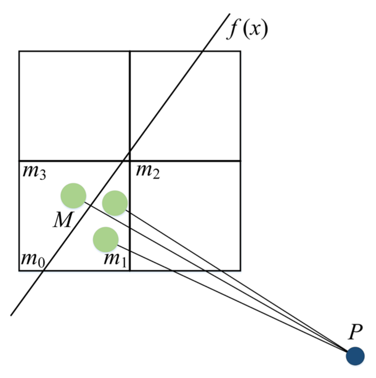
In the SDF map, the detected object contour is described using a straight line fitted to laser scan points within the same raster. The object contour is described in the SDF with the accuracy of the subgrid size. The SDF value represents the distance from the raster to the regression line, and determines the sign of the current raster. As the regression line passes through the raster, the absolute value of the calculated SDF value is smaller than the raster size, so the map is smaller than the size of the original raster. As shown in Figure 2, $m_0,m_1,m_2,m_3$ are the four vertices of a raster, Deming regression is used to fit three laser points to obtain a straight line f(x), and the distance between the midpoint of raster M and f(x) is the SDF value of raster M. The SDF value is updated to a positive value according to the raster when the distance from the raster to the unmanned vehicle position P is less than the distance from P to f(x), and the opposite SDF value is negative. The SDF map uses the average of all time measurements when updating the object contour using the SDF, thus reducing the errors caused by sensor noise. A weighted distance method is used in the 3D reconstruction [35], and the SDF map is weighted for each update in order to reduce the effects of noise and smooth the updated values.

In the W-SDF map, each time the distance between the regression line and grid is updated, the determination of whether the grid is occupied or not is made according to the sign of the SDF value inside each vertex of the grid. If each vertex of a grid is positive or negative, the grid is always on the side of one of the regression lines, i.e., there is no obstacle in this grid. In other cases, there may be an obstacle in the grid. The W-SDF map uses distance weighting for each update based on the current weight of the grid w and updated value d. The rules for calculating the weight w are as follows:

$$w=\left[\frac{\frac{1}{d^2}-\frac{1}{d^2{}_{\max }}}{\frac{1}{d^2{}_{\min }}-\frac{1}{d^2{}_{\max }}}\right]·W_{\max }$$

(1)

In Equation (1), $d_{\min }$ and $d_{\max }$ are the upper and lower limits of distance d, respectively, and $W_{\max }$ is the maximum value of the weight. The current maximum update weight is $W_{last\_\max }$. If $w\ge r\%\times W_{last\_\max }$, an update is performed; otherwise, it is not.

The rule can be updated at any time, as shown in Equation (2), as follows:

$$\left\{\begin{array}{c}{D}_{t+1}=\frac{W_t{D}_t+w_{t+1}{d}_{t+1}}{W_t+w_{t+1}}\\ W_{t+1}=W_t+w_{t+1}\end{array}\right.$$

(2)

To prevent $W_{\max }$ from reaching the upper limit too quickly, $w_{t+1}=1$ is usually set.

In the Hector SLAM algorithm, a Gaussian–Newton method is used to solve the operational scan-matching problem. If the unmanned vehicle position pose $q=\left(T,\theta \right)$ at a certain moment, T is the relative translation between the current pose and the previous pose of the robot, and $\theta$ is the relative rotation angle between the current pose and the previous pose of the robot, the scan-matching of the W-SDF map is defined as follows [14]:

$$q^{\ast }=\underset{q}{\arg \min }{\displaystyle \sum _{i=1}^n{\left[M\left(S_i\left(q\right)\right)\right]}^2}$$

(3)

$S_i=R\left(\theta \right)\cdot d_i+T$ in Equation (3) represents the world coordinates of the endpoint $d_i$ where the unmanned vehicle is currently scanned at the positional pose q, $R\left(\theta \right)$ is the rotation matrix. Equation (3) is used to identify the unmanned vehicle’s positional changes in the adjacent time when the SDF value is minimal. Hessian matrix for H. The scan-matching is first solved using the Gaussian–Newton method, as follows:

$$\Delta q=H^{-1}g$$

(4)

$$H={\left[\nabla M\left(S_i\left(q\right)\right)\frac{\partial S_i\left(q\right)}{\partial q}\right]}^T\left[\nabla M\left(S_i\left(q\right)\right)\frac{\partial S_i\left(q\right)}{\partial q}\right]$$

(5)

$$\frac{\partial S_i\left(q\right)}{\partial q}=\left[\begin{array}{cc}1& \begin{array}{cc}\begin{array}{cc}0& -s_{i,y}\sin \phi \end{array}& -s_{i,y}\cos \phi \end{array}\\ 0& \begin{array}{cc}\begin{array}{cc}1& s_{i,x}\cos \phi \end{array}& -s_{i,x}\sin \phi \end{array}\end{array}\right]$$

(6)

$$g={\displaystyle \sum _{i=1}^n{\left[\nabla M\left(S_i\left(q\right)\right)\frac{\partial S_i\left(q\right)}{\partial q}\right]}^T\left[1-M\left(S_i\left(q\right)\right)\right]}$$

(7)

If there are no obstacles in the raster, the bilinear interpolation method solves for the SDF map values and derivatives.

$$M\left(d_i\right)\approx \left|y\left(m_{3}x+m_2\left(1-x\right)\right)+\left(1-y\right)\left(m_{1}x+m_0\left(1-x\right)\right)\right|$$

(8)

$$\nabla M\left(d_i\right)\approx \left[\begin{array}{cc}y& 1-y\\ x& 1-x\end{array}\right]•\left[\begin{array}{cc}{m}_3-m_2& m_2-m_0\\ m_1-m_0& m_3-m_1\end{array}\right]$$

(9)

If there are obstacles in the raster, it is necessary to solve for a similarity value of the map gradient using the distance between the orthogonal projection h on the regression line and the corresponding axis in $d_i$, so that the map value can be approximated as the Euclidean distance between the two.

$$\left\{\begin{array}{c}\nabla M\left(d_i\right)=h-d_i\\ M\left(d_i\right)=\left|h-d_i\right|\end{array}\right.$$

(10)

As the H-matrix calculated by the Gaussian–Newton method is only semi-positive, it is singular, resulting in poor incremental stability and non-convergence of the algorithm. When the solution step $\Delta q$ is large, it appears that some approximations are not sufficiently accurate. Therefore, the L–M method is chosen to solve Equation (3).

The L–M algorithm must set a trustable maximum displacement s from an initial positional point and find the final correct displacement by taking the present positional point as the center and s as the radius in the region where the objective function is the optimal solution of a quadratic approximation function. The objective function is calculated according to the result of the solution. If the displacement can be trusted, the iteration will continue according to this rule; otherwise, the range of the trust region will be reduced, the result will be discarded, and the solution process will be started again.

Using the L–M method, the solution to Equation (3) is obtained as follows:

$$\Delta q={\left(H+\mu I\right)}^{-1}g$$

(11)

In Equation (11), $\mu$ is a penalty factor used to dynamically select the trust region range. During the iteration, if the solution $\Delta q$ decreases the objective function, the increment can be accepted and $\mu$ will be smaller with it for the next iteration; otherwise, it must be solved again. This process is repeated until the value of the objective function is minimized or the number of iterations is reached. The ratio of the objective function in the actual reduction $\Delta F$ to the estimated reduction $\Delta L$($q=\frac{\Delta F}{\Delta L}$) must be considered to discern the effective quality of its step.

If $q>0$, this iteration is considered valid, and the penalty factor is reduced.

$$\left\{\begin{array}{l}\mu =\mu •\max \left\{\frac{1}{3},1-{\left(2q-1\right)}^3\right\}\\ v=2\end{array}\right.$$

(12)

If $q\le 0$, this iteration is considered invalid, and a penalty factor is added.

$$\left\{\begin{array}{c}\mu =\mu •v\\ v=2•v\end{array}\right.$$

(13)

The L–M method can guarantee non-singularity in the $H+\mu I$ matrix based on the trust domain. If the value of $\mu$ is small, $\Delta q$ is close to the direction of the Gaussian– Newton method, and if the value of $\mu$ is relatively large, $\Delta q$ is close to the direction of the gradient reduction. The L–M method can control the step value of repeated iterations according to $\mu$, representing an effective combination of gradient reduction and the Gaussian–Newton method for making the step size of each iteration of descent more accurate and reducing the situations in which the objective function falls into local minima. When stepping out of predefined or when there are not enough available scan points in a grid, regression should be performed with scan points located in adjacent grids.

3.2. Ground Constraint Factor

In multiple environments, ground unevenness causes jitters in unmanned vehicle motion and motion interference on other dimensions of unmanned vehicle poses. Thus, the z-axis displacement of the key frames needs to add ground constraints, as these can provide more constraint information to reduce the cumulative error and improve the pose estimation accuracy. Accurate extraction of road information and complete plane segmentation in the shortest time is a key issue in establishing ground constraints; therefore, a robust estimation method with a strong anti-interference ability and fewer iterations, i.e., random sampling consistency (RANSAC), is chosen. Based on the basic principle of RANSAC, a plane is obtained by selecting any three points from each frame of the point cloud. The commonly used plane equation is $ax+by+cz=d$, where $a^2+b^2+c^{2}1$ and $d>0$,the plane normal vector is $\left(a,b,c\right)$, and the distance from the LIDAR system to the plane is d. These four parameters can determine a plane.

When the unmanned vehicle passes over an uneven road surface, the constructed pose map constraints cannot be used by fixing the plane as nodes. A subgraph-based ground extraction method is proposed to ensure that the constructed constraints are consistent with the actual situation. According to the constructed local point cloud map, the real plane parameters are extracted as follows: ${\pi }_m=\left[n_a,n_b,n_c,d\right]$. To improve the extraction efficiency of the road surface, the origin is taken as the current position, and the subgraph searches for the point cloud within the radius of the LIDAR measurements. According to the current moment LIDAR attitude, the ground parameters are transformed into the LIDAR coordinate system using Equations (14) and (15) as follows:

$${\left[{n^{\prime }}_a,{n^{\prime }}_b,{n^{\prime }}_c\right]}^T=R_t\cdot {\left[n_a,n_b,n_c\right]}^T$$

(14)

$$d^{\prime }=d-t_t\cdot {\left[{n^{\prime }}_a,{n^{\prime }}_b,{n^{\prime }}_c\right]}^T$$

(15)

In the above, ${{\pi }^{\prime }}_m=\left[{n^{\prime }}_a,{n^{\prime }}_b,{n^{\prime }}_c,d\right]$ denotes the ground coordinates in the LIDAR coordinate system and $\left[R_t,t_t\right]$ denotes the LIDAR bit attitude at the moment t. The error between the ground plane node and attitude node is obtained as shown in Equation (16), as follows:

$$e_{i,m}=q\left({{\pi }^{\prime }}_m\right)-q\left({\pi }_t\right)$$

(16)

$$q\left(\pi \right)=\left[\arctan \left(\frac{n_a}{n_b}\right),\arctan \left(\frac{n_c}{\left|n\right|}\right),d\right]$$

(17)

3.3. Key Frame Selection

A key frame selection strategy is deployed in this study to retain only a limited number of poses for estimation. When a point cloud is detected as a key frame, the environment map of the current frame needs to be updated. The main method is to convert the real-time point cloud information of the key frame into the world coordinate system with coordinate transformation in order to create a local map of the point cloud of the current subkey frame, and to update it according to the octree structure [36]. Based on the key frame selection criteria for a real-time point cloud, the first point cloud frame is usually selected as the key frame, and the rest are judged based on the relative positional changes between consecutive frames. Setting the pose of the $k-1$ th key frame as $T_{k-1}$ and that of the kth key frame as $T_k$, the relative positional changes of the consecutive key frames can be obtained using Equation (18).

$$\Delta T_{\mathrm{k}-1,k}=T_{k-1}^{-1}{T}_{\mathrm{k}}=\left(\begin{array}{cc}\Delta r& \Delta s\\ 0& 1\end{array}\right)$$

(18)

The rotation of the change between two consecutive key frames is denoted as $\Delta R$, the translation of the change between two consecutive key frames is denoted as $\Delta s$, and the time of the transformation between two consecutive key frames is denoted as $\Delta t$.

$$\Delta R=\arccos \left(\frac{trace\left(\Delta r\right)-1}{2}\right)$$

(19)

$$‖\Delta s‖=\sqrt{\Delta x^2+\Delta y^2+\Delta z^2}$$

(20)

$$\Delta t=t_k-t_{k-1}$$

(21)

When any of the above three criteria exceeds a set threshold, the current kth frame of the point cloud is selected as a key frame, and the other frame of the two key frames is discarded. The key frames selected using this method can keep the map density balanced with the memory loss during operation and are uniformly distributed in space, making them suitable for real-time non-linear optimisation.

4. Closure Detection

To reduce the cumulative sensor error, closed-loop detection is employed. When performing closed-loop detection, the current real-time key frames are first compared with historical key frames, and the highest-scoring key frame is selected as a candidate loopback frame. The key frames and candidate loopback frames are added as nodes in the SLAM graph optimisation, and the edge constraint is the relative pose obtained through the point cloud matching.

The algorithm for closed-loop detection is described in Algorithm 1 [37]. It is assumed that the current frame point cloud is represented in the IMU system as $P_m$ and that its relative pose change with respect to the world coordinate system is $T_m$. If the key frame database, as the set of poses $D_T$ and set of point clouds $D_P$, is not empty, a kd-tree search with a radius r is performed. This task aims to determine if a ${T^{\prime }}_m$ can be found in the key frame pose set $D_T$, such that the sum of the root mean square error of the point cloud $P_m$ of the current frame after the relative change $T_{ICP}$ and that of nearest point in $D_P$ is minimized; then, the cycle is detected. The key frame pose set $D_T$ registers the key frame point cloud $D_P$ to the local point cloud map M constructed in the world coordinate system.

Algorithm 1. Loop closure algorithm.
Input:	$T_m$ and $P_m$ from the current point cloud frame
Output:	$T_{ICP}$
1:	if $(T_m,P_m)$.isKeyframe() then
2:	if $D_T\ne \varphi$ or $D_P\ne \varphi$ then
3:	${T^{\prime }}_m\leftarrow$ KDtree.RadiusSearch $(T_m,D_T,r)$
4:	$M\leftarrow$ registerPointCloud $(D_T,D_P)$
5:	if ${T^{\prime }}_m\ne 0$ then
6:	$T_{ICP}$← ComputeICP $(P_m,M,T_m)$
7:	end if
8:	end if
9:	${T^{\prime }}_m\leftarrow$0
10:	$D_T=D_T\cup T_m$
11:	$D_P=D_P\cup P_m$
12:	end if

Only the current pose of the point cloud in the world coordinates for the current frame is obtained, and $T_{ICP}$ and M are fed back to the global optimisation for state correction.

5. Factor Graph Optimisation

5.1. Factor Graphs

In this study, we fused information from multiple constraints to obtain high-accuracy unmanned vehicle trajectories while using factor graphs to model the graph optimisation problem. The factor graph is shown in Figure 3. There are five factors in the factor graph: the a priori factor, wheel odometer and IMU factor, LiDAR odometer factor, closed-loop factor, and ground constraint factor [38].

(1)

The a priori factor is considered as the first node of the fixed pose graph; it is also considered as the origin of the world coordinate system (which is fixed by the a priori factor).

(2)

The wheel odometer and IMU coefficients are obtained from two sensors, i.e., the wheel odometer and IMU. These allow for the calculation of the relative attitude between the two key frames, and the relative attitude provides a spatial constraint between the two key frames.

(3)

The LiDAR odometry factor is derived from the front-end scan-matching module. The front-end scan-matching module calculates the relative attitude between two key frames by weighting the SDF and L–M results.

(4)

The closed-loop factor originates from the closed-loop detection module, and the validated closed-loop detection constraints are added to the factor map.

(5)

The ground constraint factor originates from the extracted ground constraint in the front-end scan-matching module, and multiple key frames are connected by the ground constraint factor.

In Figure 3, G is the ground constraint and X is the bit attitude of the unmanned vehicle. The setting factor fixes the first node of the attitude map, obtains data through the sensor, and integrates these to calculate the relative attitude between key frames in order to provide the corresponding spatial constraints; both the LiDAR odometer factor and ground constraint factor are obtained through the front-end scan matching module. Then, when a new key frame is obtained, the closed-loop module automatically performs closed-loop detection and rejects the effect of the incorrect closed-loop on simultaneous positioning and map building.

5.2. Factor Graph Elimination Optimisation

To improve the speed of the variable marginalization as well as the maximum posterior probability inference, a transformation between the factor graphs and Bayesian networks [39] needs to be accomplished using an elimination optimisation algorithm.

The factor graph Equation (22) is decomposed into the probability density of the factorized Bayesian network shown in Equation (23) through variable elimination, and into the form of Equation (24) for all factors in the least-squares problem.

$$\varphi \left(X\right)=\varphi \left(x_1,x_2,x_3,\cdots ,x_n\right)$$

(22)

$$p\left(X\right)=p\left(x_1\left|S_1\right.\right)p\left(x_2\left|S_2\right.\right)p\left(x_3\left|S_3\right.\right)\cdots p\left(x_n\left|S_n\right.\right)=\prod _{j}p\left(x_j\left|S_j\right.\right)$$

(23)

$${\varphi }_i\left(X_i\right)=\exp \left\{-\frac{1}{2}{‖A_i{X}_i-b_i‖}_2^2\right\}$$

(24)

In Equation (24), $A_i$ consists of the small sub-blocks corresponding to each variable.

The following is the algorithm used to eliminate the variable $x_j$ from the factor graph ${\mathrm{\Phi }}_{j:n}$ [40]

(1)

Remove all factors ${\varphi }_i\left(X_i\right)$ adjacent to $x_j$.

(2)

Generate the separator $S\left(x_j\right)$ (all variables associated with ${\varphi }_i\left(X_i\right)$ except $x_j$).

(3)

Generate the product factor ${\prod }_i{\varphi }_i\left(X_i\right)\to \psi \left(x_j,S_j\right)$.

(4)

Decompose the product $\psi \left(x_j,S_j\right)\to p\left(x_j\left|S_j\right.\right)\tau \left(S_j\right)$.

(5)

Add a new factor $\tau \left(S_j\right)$ at the end of the factor graph.

Because the partial QR decomposition is related to the linearization factor, the augmented matrix $\left[{\overline{A}}_j\left|{\overline{b}}_j\right.\right]$ corresponding to the product factor $\psi \left(x_j,S_j\right)$ is converted using the partial QR decomposition as follows:

$$\left[{\overline{A}}_j\left|{\overline{b}}_j\right.\right]=Q\left[\begin{array}{c}\begin{array}{ccc}{R}_j& T_j& d_j\end{array}\\ \begin{array}{ccc}& {\tilde{A}}_{\tau }& {\tilde{b}}_{\tau }\end{array}\end{array}\right]$$

(25)

In Equation (25), $R_j$ is the upper triangular matrix.

Multiplying the two parametrics of a vector and the rotation matrix Q does not change the properties of the vector; $\psi \left(x_j,S_j\right)$ is replaced by the product of the two factors.

$$\psi \left(x_j,S_j\right)=\exp \left\{-\frac{1}{2}{‖{\overline{A}}_j\left[x_j;S_j\right]-{\overline{b}}_j‖}_2^2\right\}=p\left(x_j\left|S_j\right.\right)\tau \left(S_j\right)$$

(26)

Conventional factor graph algorithms fuse only the information of the previous moment; this leads to the loss of most of the information and decreases the anti-interference and state estimation abilities. Therefore, we add a sliding window to the chain factor graph, and use the moments outside the window as a priori information. The number of states is denoted by N.

First, the new factor nodes are added to the original factor graph at the new sampling moment, and the sliding window is slid to the right to contain the new factor nodes. Second, the state variables outside the sliding window are considered as prior information, and the state variables from the previous moment are computed sequentially to the latest moment using the elimination optimisation algorithm. Finally, the Gaussian–Newton iteration is used to find the optimal state estimate.

If N = 3, Figure 4, Figure 5 and Figure 6 show the calculation steps of the algorithm (the factor nodes are the black points).

In a front-to-back order, the state information of $x_2$ is first passed to $x_3$ as a priori information and $x_3$ is eliminated. The result is shown in Figure 5, where “☆” indicates the new factor node $\tau \left(S_3\right)$ obtained through the partial QR decomposition.

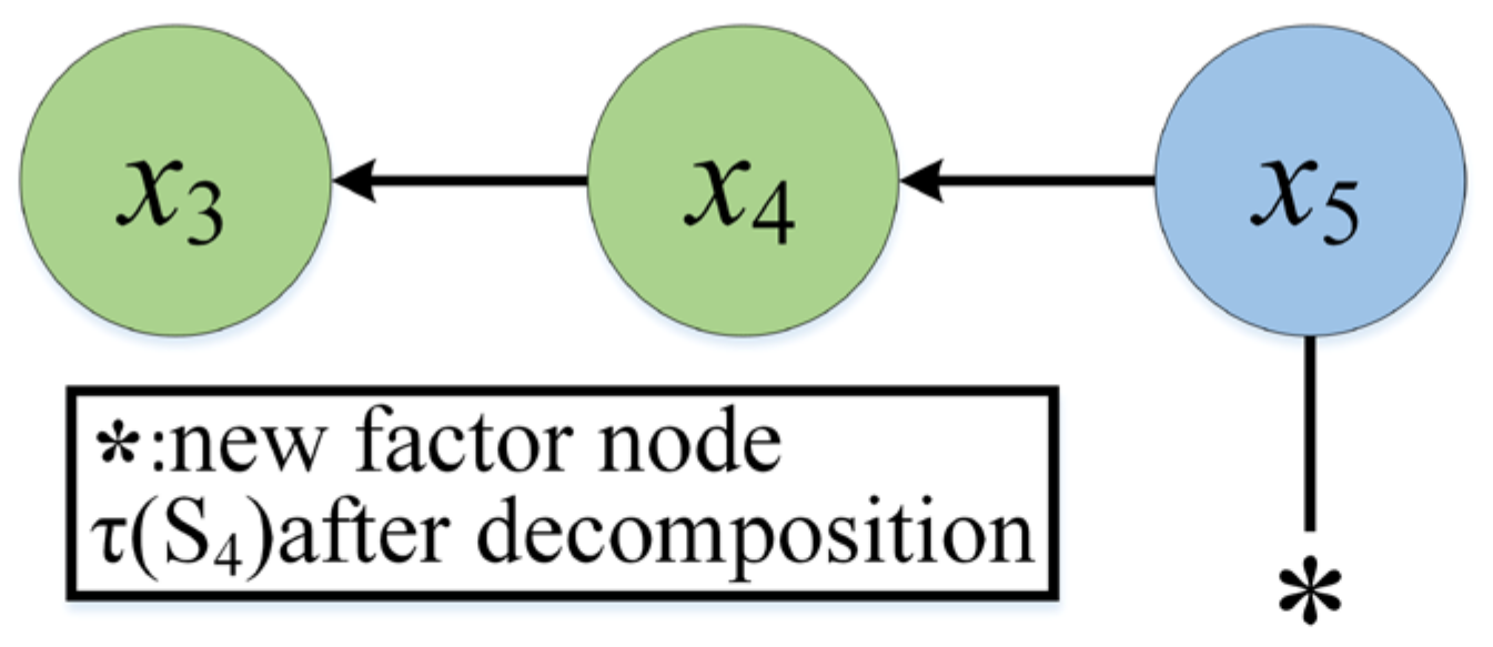
After marginalizing $x_3$, the elimination of the elements for $x_4$ is shown in Figure 6; “*” indicates that the new factor node $\tau \left(S_4\right)$ is obtained using the partial QR decomposition.

The maximum a posteriori probability estimate of $x_5$ is obtained by marginalizing $x_4$. In this system, the sliding window follows the new factor node joining to the right and repeats the above steps to obtain the maximum a posteriori probability estimate for the new state quantity. Compared to a direct solution, this method can avoid the operation of a high-dimensional number matrix and significantly improve the operation speed.

6. Experiments

The experimental platform in this study is an autonomous unmanned vehicle with sensors consisting of an RS-LiDAR-16, IMU, and wheeled odometer, as shown in Figure 7. The map was created by an IPC with processor model Intel i5-10210U1.60 GHz memory of 8 G. The framework was entirely based on the C++ programming language, and the operating system is Ubuntu 18.04.6LTS. The resolution of the map is determined by the size of the raster in the map when using the occupied raster map as the map model; the W-SDF map is an improved map based on the occupied raster map; therefore, the map resolution (raster size) is 0.05 m for the experiments in this paper. For safety and reliability during the experiments, the unmanned vehicle was operated at a uniform speed of 4 m/s during the experiments of various algorithms.

To test the accuracy, robustness, and timeliness of the proposed SLAM algorithm framework, the complex environment of an office building outdoor (60 × 70) and a non-motorized vehicle car park straight road (about 30 m long) was chosen. First, the front-end optimisation was compared with the existing Hector and Cartographer algorithms [41] to verify the effectiveness and robustness of the proposed algorithm, i.e., by comparing the map building, localisation accuracy, and memory usage.

6.1. Front-End Experiments

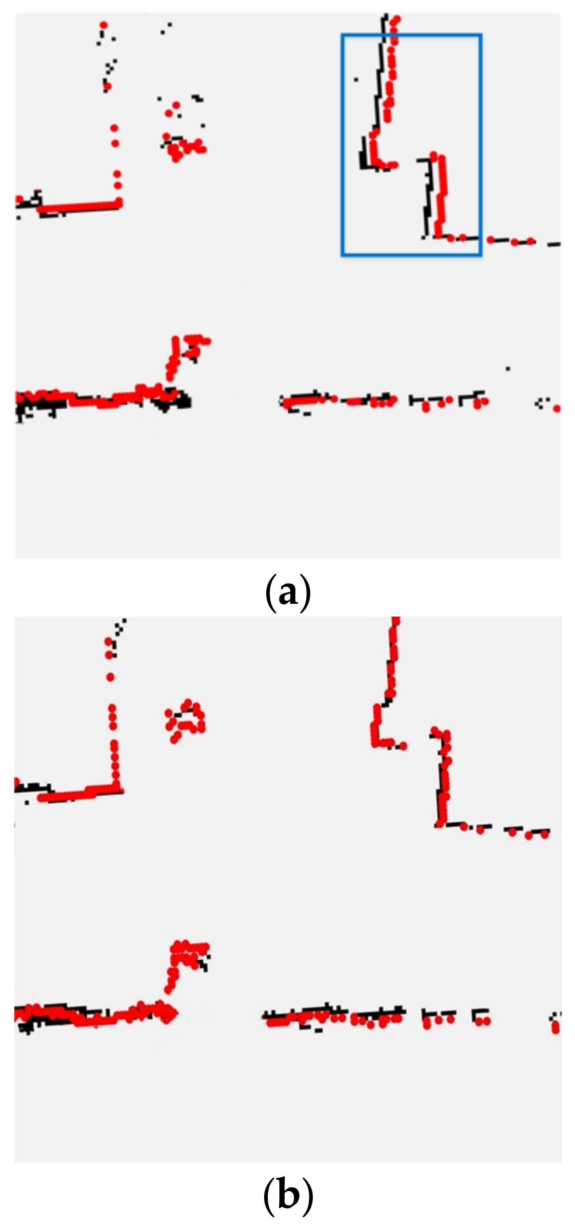
To better validate the proposed scan-matching algorithm, this section describes an experimental comparison between the Hector algorithm and the algorithm proposed herein. Based on scan-matching of the same environment (a T-shaped intersection), Figure 8 shows the results from the two methods Figure 8a,b) show the results from the Hector algorithm and scan-matching algorithm proposed herein to build the maps, respectively).

As can be seen from Figure 8a, black is the previous frame and red is the current frame (laser scan point) for the experimental results of the Hector algorithm map. The blue box marks an obvious misalignment phenomenon in the T-shaped intersection corner walls, while, in the proposed algorithm to scan the wall, a misalignment phenomenon does not appear, which can be obviously observed in Figure 8b, making scan matching more accurate and complete. The experimental results show that the proposed algorithm can better build the scan-matching map in an actual scenario.

6.2. Closed-Loop Detection and Back-End Experiments

To demonstrate the map-building capabilities of the algorithm, experiments were conducted in an outdoor promenade-type environment and complex laboratory environment on the periphery of a large building. The following is the experimental results’ diagram: in the red circle in the gray part of the unidentified area, dark blue is the obstacle and white is the ground.

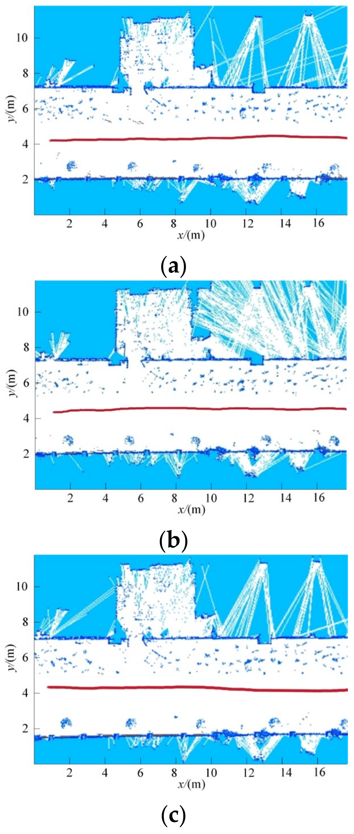
The first scene was a non-motorized parking promenade, shown in Figure 9a. By collecting similar promenade information and without using a tight wall as a constraint, the SLAM building map was expected to present greater difficulties, as the map would be prone to certain scenes that could not be identified or that missed detection. As such, this experiment was a good test of the recognition ability and stability of the proposed algorithm, along with those from the Hector and Cartographer algorithms.

According to the results shown in the figures, it can be seen from Figure 9b,c that there are evident unrecognized areas and more confusing burrs from the other two approaches, whereas the maps built by the proposed algorithm (shown in (d) are more regular and do not show the situations that occur in the above two algorithms.

To further verify a more complex environment, an experimental real-world view around an office building is shown in Figure 10a. As the map area was large and the ground was not flat, the performance of the algorithms for closed-loop detection and the ground constraint could be tested more accurately. The experimental results are shown in Figure 10.

From Figure 10b,c, it can be seen that in the experimental environment with more obstacles and complexities, there are unrecognized areas in the maps built using the Hector and Cartographer algorithms (marked with red ellipse circles), the ground and obstacle recognition situation appears blurred, and there are also some burrs that interfere with the map building. The experimental results show that the proposed algorithm can correctly identify the scenes and significantly improve the algorithm’s robustness.

6.3. Data Analysis and Comparison

6.3.1. Trajectory Error Analysis

(1)

Promenade test scenes

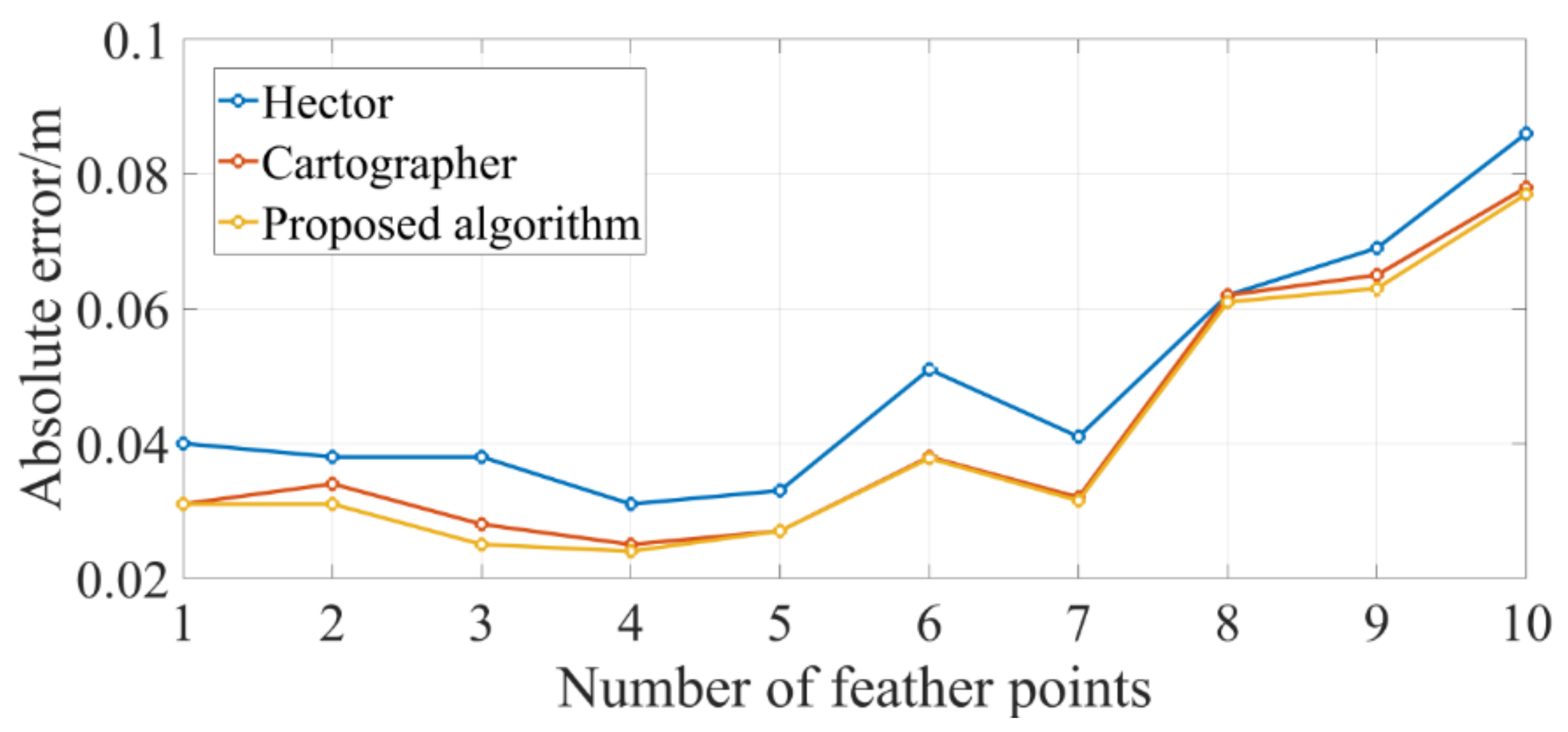
To further reflect the accuracy of the algorithm, a promenade test scene was conducted. The driving trajectory is shown in Figure 11 as a red line. Ten feature points on the driving path of the unmanned vehicle were selected for error analysis, and the results are shown in

Table 1. Error analysis of the three algorithms in the promenade environment.

Parameter	Hector	Cartographer	Proposed Algorithm
Max error/m	0.0860	0.0780	0.0770
Min error/m	0.0310	0.0250	0.0240
Mean absolute error(MAE)/m	0.0489	0.0420	0.0408

.

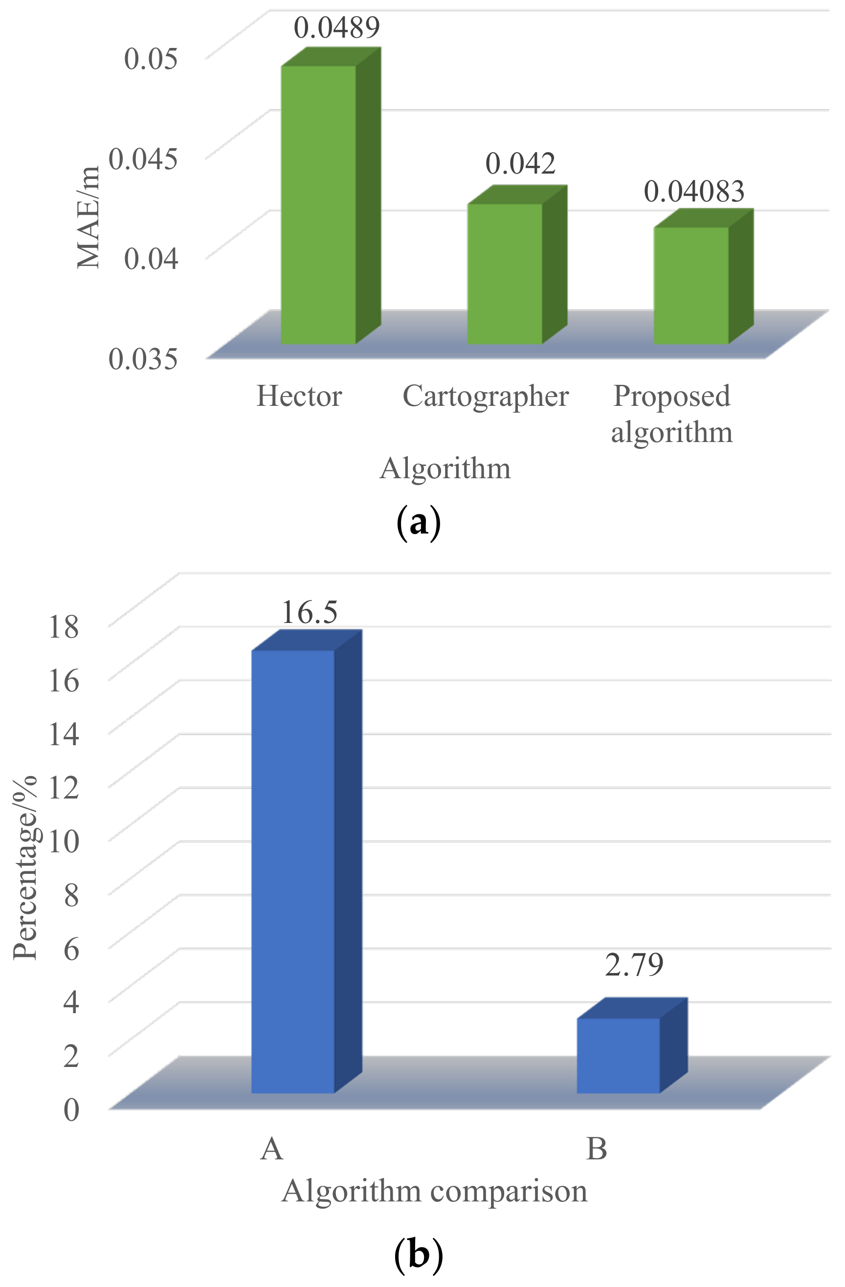
In the outdoor promenade environment, all three algorithms show good performance. The absolute errors of the three algorithms are calculated as shown in Figure 12, but the error of the proposed algorithm in this paper is significantly lower than the error of the other two algorithms, which is more favorable as regards accuracy when building the map. A specific error comparison is shown in Figure 13, which shows that the error of the proposed SLAM algorithm in building the map is reduced by 2.79% compared with the Cartographer algorithm and by 16.50% compared with the Hector algorithm.

(2)

Office building test scenario

To test the performance of the proposed algorithm on complex and uneven roads, experiments were conducted in an office building. Figure 14 shows the driving trajectory outside the office building. The same 10 points were selected for error analysis, and the results are shown in

Table 2. Error analysis of the three algorithms in the office building.

Parameter	Hector	Cartographer	Proposed Algorithm
Max error/m	0.0270	0.0250	0.0245
Min error/m	0.0200	0.0170	0.0165
Mean absolute error(MAE)/m	0.0234	0.0217	0.0181

.

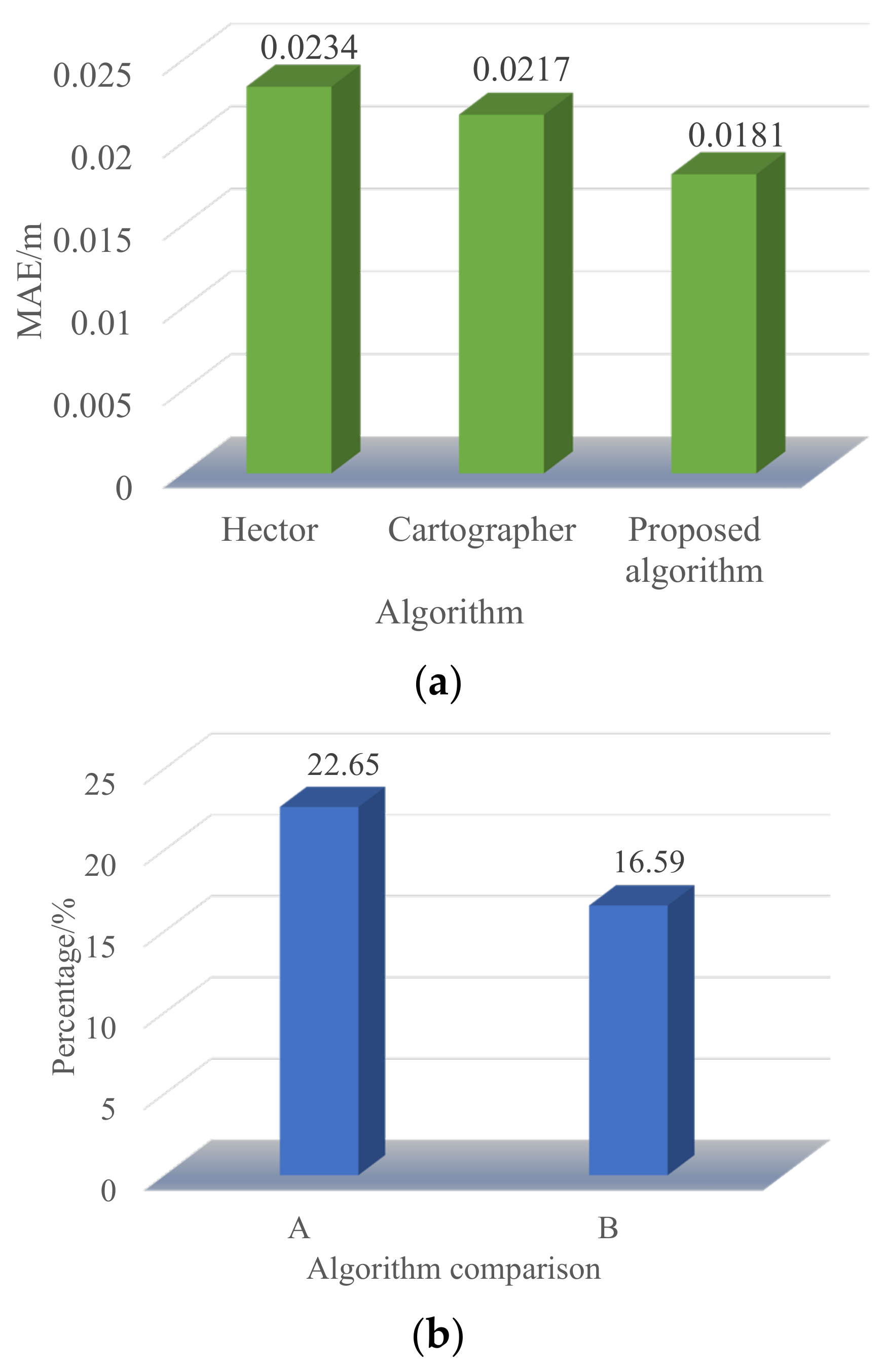
In the experimental office building scenario, all three algorithms show a better map-building effect. The absolute errors of the calculations are shown in Figure 15, indicating that the proposed algorithm has higher accuracy than the other two algorithms, reflecting the adaptability of the algorithm of this paper to various environments. A specific error comparison is shown in Figure 16, in which we can see that the error of the proposed SLAM algorithm is reduced by 16.59% compared with the Cartographer algorithm and by 22.65% compared with the Hector algorithm.

6.3.2. Memory Occupancy Analysis

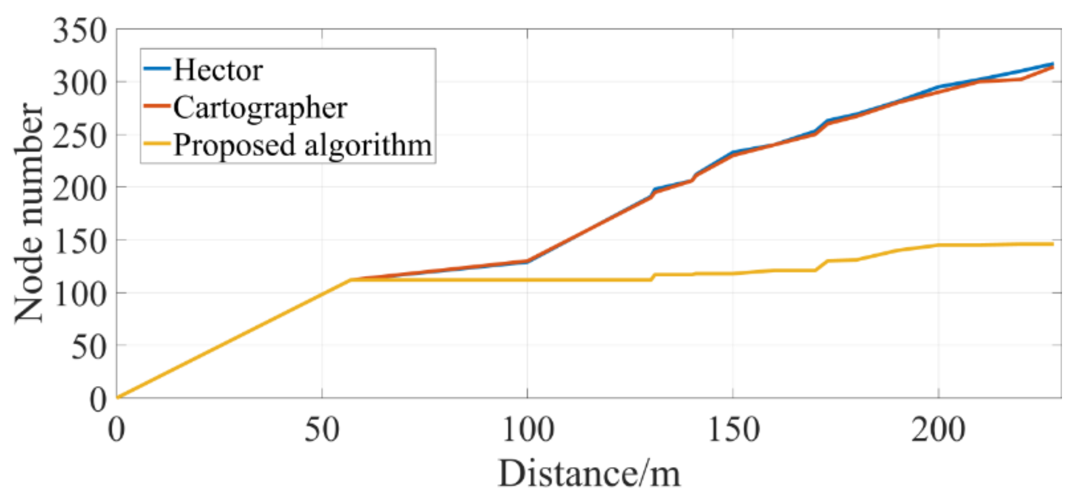
Figure 17 shows the relationship between the number of nodes and the running distance when the office building map is built. To verify the effectiveness of the algorithm selection strategy, the numbers of nodes in the bit-posture map during the operations of the three algorithms were extracted. Figure 17 shows that the number of nodes in the Hector and Cartographer methods increases with the length of the unmanned vehicle trajectory. However, the number of nodes tends to stabilize after the unmanned vehicle travels a certain distance. When the distance traveled by the unmanned vehicle increases, the memory occupation of the Hector and Cartographer keeps increasing, and all the memory can become occupied when building a larger map. This does not happen with the proposed method. The experimental results show that the proposed factor graph elimination optimisation can significantly reduce the memory occupancy of the algorithm and improve the computational efficiency and stability of the algorithm.

7. Conclusions

In this paper, we proposed a multi-sensor fusion method based on factor map elimination optimisation for 2D-SLAM in multiple scenes. The main research content is as follows:

(1)

Introducing a weighted SDF map and adding ground constraints, the L–M method is used to solve for reduced localisation errors, improved matching accuracy of front-end scan matching and robustness on uneven road surfaces.

(2)

Combining closed-loop detection and keyframing enables optimal closed-loop detection in the shortest possible time.

(3)

The proposed factor graph elimination algorithm adds a sliding window to the chain factor graph model to retain the historical state information within the window and improve the fault tolerance. In order to avoid high-dimensional matrix operations, the elimination algorithm is introduced to transform the factor graph into a Bayesian network, which sequentially marginalizes the historical states to achieve matrix dimensionality reduction and reduce the memory occupation rate.

In this paper, experiments are conducted on an unmanned vehicle, in which the map building capability and localisation accuracy of different SLAM algorithms are evaluated and the memory usage of these algorithms is analyzed, and the experimental data verify the effectiveness of the proposed SLAM algorithm. The experimental data verifies the effectiveness of the proposed SLAM algorithm, which can be of good practical value in real applications.

In the future, we will continue to improve the algorithm in this paper to make the SLAM algorithm faster and enhance its robustness. The semantic information of point cloud will be studied, and the fusion of visual sensors will be added appropriately to adapt in order to more complex scenes.

References

1. Wang, L.; Cai, Z.X. Progress of CML for mobile robots in unknown environments. Robot 2004, 26, 380–384. [Google Scholar] [CrossRef]
2. Zou, Q.; Sun, Q.; Chen, L.; Nie, B.; Li, Q.Q. A Comparative Analysis of LiDAR SLAM-Based Indoor Navigation for Autonomous Vehicles. IEEE Trans. Intell. Transp. Syst. 2022, 23, 6907–6921. [Google Scholar] [CrossRef]
3. Mac, T.T.; Lin, C.Y.; Huan, N.G.; Nhat, L.D.; Hoang, P.C.; Hai, H.H. Hybrid SLAM-based Exploration of a Mobile Robot for 3D Scenario Reconstruction and Autonomous Navigation. Acta Polytech. Hung. 2021, 18, 197–212. [Google Scholar]
4. Gupta, A.; Fernando, X. Simultaneous Localization and Mapping (SLAM) and Data Fusion in Unmanned Aerial Vehicles: Recent Advances and Challenges. Drones 2022, 6, 85. [Google Scholar] [CrossRef]
5. Song, J.E.; Joongjin, K. Building a Mobile AR System based on Visual SLAM. J. Semicond. Disp. Technol. 2021, 20, 96–101. [Google Scholar]
6. Kuo, C.Y.; Huang, C.C.; Tsai, C.H.; Shi, Y.S.; Smith, S. Development of an immersive SLAM-based VR system for teleoperation of a mobile manipulator in an unknown environment. Comput. Ind. 2021, 132, 103502. [Google Scholar] [CrossRef]
7. Lepej, P.; Rakun, J. Simultaneous localisation and mapping in a complex field environment. Biosyst. Eng. 2016, 150, 160–169. [Google Scholar] [CrossRef]
8. Li, C.Y.; Peng, C.; Zhang, Z.Q.; Miao, Y.L.; Zhang, M.; Li, H. Positioning and map construction for agricultural robots integrating odometer information. Trans. Chin. Soc. Agric. Eng. 2021, 37, 16–23. [Google Scholar] [CrossRef]
9. Dwijotomo, A.; Rahman, M.A.; Ariff, M.H.M.; Zamzuri, H.; Azree, W.M.H.W. Cartographer SLAM Method for Optimization with an Adaptive Multi-Distance Scan Scheduler. Appl. Sci. 2020, 10, 347. [Google Scholar] [CrossRef] [Green Version]
10. Singh, P.; Jeon, H.; Yun, S.; Kim, B.W.; Jung, S.Y. Vehicle Positioning Based on Optical Camera Communication in V2I Environments. CMC Comput. Mater. Contin. 2022, 72, 1927–2945. [Google Scholar] [CrossRef]
11. Pedrosa, E.; Pereira, A.; Lau, N. A Non-Linear Least Squares Approach to SLAM using a Dynamic Likelihood Field. J. Intell. Robotic Systems 2019, 93, 519–532. [Google Scholar] [CrossRef]
12. Ding, Y.H.; Wu, H.Y.; Chen, Y. SLAM method based on 2D laser scan-to-submap matching. Comput. Eng. Des. 2020, 41, 3458–3463. [Google Scholar] [CrossRef]
13. Jiang, G.L.; Yin, L.; Liu, G.D.; Xi, W.N.; Ou, Y.S. FFT-Based Scan-Matching for SLAM Applications with Low-Cost Laser Range Finders. Appl. Sci. - 2019, 9, 41. [Google Scholar] [CrossRef] [Green Version]
14. Ren, R.K.; Fu, H.; Wu, M. Large-Scale Outdoor SLAM Based on 2D Lidar. Electronics 2019, 8, 613. [Google Scholar] [CrossRef] [Green Version]
15. Liang, S.; Cao, Z.Q.; Wang, C.P.; Yu, J.Z. A Novel 3D LiDAR SLAM Based on Directed Geometry Point and Sparse Frame. IEEE Robot. Autom. Lett. 2021, 6, 374–381. [Google Scholar] [CrossRef]
16. Marchel, L.; Specht, C.; Specht, M. Testing the Accuracy of the Modified ICP Algorithm with Multimodal Weighting Factors. Energies 2020, 13, 5939. [Google Scholar] [CrossRef]
17. Li, X.Y.; Ling, H.B. Hybrid Camera Pose Estimation With Online Partitioning for SLAM. IEEE Robot. Autom. Lett. 2020, 5, 1453–1460. [Google Scholar] [CrossRef]
18. Xu, Y.; An, W.F. RGB-D SLAM System Based on BA Optimization and KL Divergence. J. Northeast. Univ. Nat. Sci. 2020, 41, 933–937. [Google Scholar] [CrossRef]
19. Liu, Z.; Zhang, F. BALM:Bundle Adjustment for Lidar Mapping. IEEE Robot. Autom. Lett. 2021, 6, 3184–3191. [Google Scholar] [CrossRef]
20. Fossel, J.D.; Tuyls, K.; Sturm, J. 2D-SDF-SLAM: A signed distance function based SLAM frontend for laser scanners. In Proceedings of the 2015 IEEE/RSJ International Conference on Intelligent Robots and Systems (IROS), Hamburg, Germany, 28 September–3 October 2015; pp. 1949–1955. [Google Scholar] [CrossRef]
21. Wang, Z.L.; Li, W.Y. Moving Objects Tracking and SLAM Method Based on Point Cloud Segmentation. Robot 2021, 43, 177–192. [Google Scholar] [CrossRef]
22. Wen, J.R.; Qian, C.; Tang, J.; Liu, H.; Ye, W.F.; Fan, X.Y. 2D LiDAR SLAM Back-End Optimization with Control Network Constraint for Mobile Mapping. Sensors 2018, 18, 3668. [Google Scholar] [CrossRef] [Green Version]
23. Zhang, H.K.; Chen, N.S.; Dai, Z.X.; Fan, G.Y. A Multi-level Data Fusion Localization Algorithm for SLAM. Robot 2021, 43, 641–652. [Google Scholar] [CrossRef]
24. Jiang, S.K.; Wang, S.L.; Yi, Z.Y.; Zhang, M.N.; Lv, X.L. Autonomous Navigation System of Greenhouse Mobile Robot Based on 3D Lidar and 2D Lidar SLAM. Front. Plant Sci. 2022, 13, 815218. [Google Scholar] [CrossRef] [PubMed]
25. Wang, X.B.; Li, X.X.; Liao, J.C.; Feng, S.Q.; Li, S.Y.; Zhou, Y.X. Tightly-coupled stereo visual-inertial-LiDAR SLAM based on graph optimization. Acta Geod. Et Cartogr. Sin. 2022, 51, 1744–1756. [Google Scholar] [CrossRef]
26. Fang, X.; Wang, C.; Nguyen, T.M.; Xie, L.H. Graph Optimization Approach to Range-Based Localization. IEEE Trans. Syst. Man Cybern. Syst. 2021, 51, 6830–6841. [Google Scholar] [CrossRef] [Green Version]
27. Dai, T.; Miao, L.J.; Shao, H.J. A Multi-beam Sonar-based Graph SLAM Method. Acta Armamentarii 2020, 41, 1384–1392. [Google Scholar] [CrossRef]
28. Li, B.Y.; Liu, S.J.; Cui, M.Y.; Zhao, Z.H.; Huang, K. Multi-Vehicle Collaborative SLAM Framework for Minimum Loop Detection. Acta Electron. Sin. 2021, 49, 2241–2250. [Google Scholar] [CrossRef]
29. Joan, V.; Joan, S.; Juan, A.C. Pose-graph SLAM sparsification using factor descent. Robot. Auton. Syst. 2019, 119, 108–118. [Google Scholar] [CrossRef] [Green Version]
30. Bai, S.Y.; Lai, J.i.Z.; Lv, P.; Ji, B.W.; Zheng, X.Y.; Fang, W.; Cen, Y.T. Mobile Robot Localization and Perception Method for Subterranean Space Exploration. Robot 2022, 44, 463–470. [Google Scholar] [CrossRef]
31. Joan, V.; Joan, S.; Juan, A.C. Graph SLAM Sparsification With Populated Topologies Using Factor Descent Optimization. IEEE Robot. Autom. Lett. 2018, 3, 1322–1329. [Google Scholar] [CrossRef] [Green Version]
32. Huang, Q.Q.; Papalia, A.; Leonard, J.J. Nested Sampling for Non-Gaussian Inference in SLAM Factor Graphs. IEEE Robot. Autom. Lett. 2022, 7, 9232–9239. [Google Scholar] [CrossRef]
33. Fan, S.W.; Zhang, Y.; Hao, Q.; Jiang, P.; Yu, F. Cooperative positioning and error estimation algorithm based on factor graph. Syst. Eng. Electron. 2021, 43, 499–507. [Google Scholar] [CrossRef]
34. Yang, L.; Ma, H.W.; Wang, Y.; Xia, J.; Wang, C.W. A Tightly Coupled LiDAR-Inertial SLAM for Perceptually Degraded Scenes. Sensors 2022, 22, 3063. [Google Scholar] [CrossRef]
35. Hemmat, H.J.; Bondarev, E.; de With, P.H.N. Exploring Distance-Aware Weighting Strategies for Accurate Reconstruction of Voxel-Based 3D Synthetic Models. Lect. Notes Comput. Sci. 2014, 8325, 412–423. [Google Scholar] [CrossRef]
36. Hornung, A.; Wurm, K.M.; Bennewitz, M.; Stachniss, C.; Burgard, W. OctoMap: An efficient probabilistic 3D mapping framework based on octrees. Auton. Robot. 2013, 34, 189–206. [Google Scholar] [CrossRef] [Green Version]
37. Yang, J.C.; Lin, C.J.; You, B.Y.; Yan, Y.L.; Cheng, T.H. RTLIO: Real-Time LiDAR-Inertial Odometry and Mapping for UAVs. Sensors 2021, 21, 3955. [Google Scholar] [CrossRef]
38. Huang, S.; Huang, H.Z.; Zeng, Q.; Huang, P. A Robust 2D Lidar SLAM Method in Complex Environment. Photonic Sens. 2022, 14, 220416. [Google Scholar] [CrossRef]
39. Indelman, V.; Williams, S.; Kaess, M.; Dellaert, F. Information fusion in navigation systems via factor graph based incremental smoothing. Robot. Auton. Syst. 2013, 61, 721–738. [Google Scholar] [CrossRef]
40. Gao, J.Q.; Tang, X.Q.; Zhang, H.; Wu, M. Vehicle INS/GNSS/OD integrated navigation algorithm based on factor graph. Syst. Eng. Electron. 2018, 40, 2547–2553. [Google Scholar] [CrossRef]
41. Trejos, K.; Rincon, L.; Bolanos, M.; Fallas, J.; Marin, L. 2D SLAM Algorithms Characterization, Calibration, and Comparison Considering Pose Error, Map Accuracy as Well as CPU and Memory Usage. Sensors 2022, 22, 6903. [Google Scholar] [CrossRef]
Figure 1. Framework of simultaneous location and mapping (SLAM) system.
Sustainability 15 01172 g001
Figure 2. Weighted signed distance function (W-SDF) map principle.
Sustainability 15 01172 g002
Figure 3. Factor graph model.
Sustainability 15 01172 g003
Figure 4. Adding a sliding window to the chain factor diagram.
Sustainability 15 01172 g004
Figure 5. Factor graph after elimination of x 3 .
Sustainability 15 01172 g005
Figure 6. Factor graph at the end of elimination.
Sustainability 15 01172 g006
Figure 7. Test platform. The test platform built has three types of sensors: LIDAR, IMU and wheel odometry.
Sustainability 15 01172 g007
Figure 8. Scan-matching result. (a) Hector (b) Proposed algorithm.
Sustainability 15 01172 g008
Figure 9. The actual view of the promenade and the experimental results. (a) Actual view of the promenade (b) Hector (c) Cartographer (d) Proposed algorithm.
Sustainability 15 01172 g009
Figure 10. The actual view of the office building and the experimental results. (a) Office building view (b) Hector (c) Cartographer (d) Proposed algorithm.
Sustainability 15 01172 g010aSustainability 15 01172 g010b
Figure 11. Promenade trajectory (a) Hector (b) Cartographer (c) Proposed algorithm.
Sustainability 15 01172 g011
Figure 12. Promenade three algorithm error curves.
Sustainability 15 01172 g012
Figure 13. Promenade error variation diagram. (a) Comparison of mean absolute errors (b) Comparison of algorithm enhancement (A: Hector vs. proposed algorithm; B: Cartographer vs. proposed algorithm).
Sustainability 15 01172 g013
Figure 14. Office building trajectory (a) Hector (b) Cartographer (c) Proposed algorithm.
Sustainability 15 01172 g014aSustainability 15 01172 g014b
Figure 15. Error curves of the three algorithms for the office building.
Sustainability 15 01172 g015
Figure 16. Office building error variation graph. (a) Comparison of mean absolute errors (b) Comparison of algorithm enhancement (A: Hector vs. proposed algorithm; B: Cartographer vs. proposed algorithm).
Sustainability 15 01172 g016
Figure 17. Positional nodes.
Sustainability 15 01172 g017