Impact of the Variability of Vegetation, Soil Moisture, and Building Density between City Districts on Land Surface Temperature, Warsaw, Poland

Abstract

The temperature of a city’s surface is influenced by many factors, including human-dependent ones that can be shaped, such as the urban density, the condition of urban vegetation, the presence of urban water bodies, and soil moisture. Knowledge on this subject allows for improving the urban climate through better planning and construction of urban infrastructure and adapting cities to climate change and avoiding deadly heat waves increasingly threatening European cities. So far, mainly the first three factors have been studied particularly well, while there is no in-depth research on the impact of soil moisture on a city’s climate in the literature. This article fills this gap by analyzing the impact of all the abovementioned factors on the temperature of the city’s surface in Warsaw, a large European urban agglomeration, located in a temperate climate zone. Due to the exceptionally large war damage to Warsaw during World War II, rapid postwar reconstruction, and significant expansion, the city is characterized by a very large diversity of urban development density and a much larger amount of green areas compared to most large cities, such as old Western European agglomerations. The scientific novelty of the work is also the fact that the soil moisture content was analyzed using the TVDI/qTVDI (Temperature Vegetation Dryness Index Estimation) indexes obtained by using the so-called triangle methods in NDVI-LST space, based on satellite observations. Such analyses have not been performed so far in urban areas, while in the article, many new results were obtained on this subject. For example, Pearson’s correlation coefficients between LST, NDBI, NDVI, and qTVDI calculated for the entire area of Warsaw on 8 August 2020 were 0.78, 0.45, and −0.35, respectively. Another important aspect of the work is that it includes comparative studies of the impact of the abovementioned factors on the temperature of the Earth’s surface at the level of different city districts. As a result, it was possible to more effectively study the impact of the abovementioned factors on the temperature of the Earth’s surface at the scale of local administrative units. Thanks to the obtained results, urban planners will be able to reduce urban hazard risks caused by climate change.

1. Introduction

Urbanization and land conversion to urban areas represent one of the major challenges in the 21st century. It refers to the mass movement of the population from rural areas to cities.

According to the United Nations’ data, in 2019, 4.2 billion people were living in urban areas. Moreover, they claim that this number will grow rapidly, reaching 6 billion people by 2041 [1]. This fact has numerous consequences. Growing cities and city centers are undoubtedly linked to the destruction of green spaces and vegetation [2]. Among other negative effects of rapid urbanization, the most severe ones are population density excess, environmental pollution, bad urban regulations, and traffic congestion, which result in a worsening quality of life [3].

Nowadays, cities that are the product of that urbanization and people living there face very challenging problems such as climate change and heat extremes [4].

Urban heat affects residents and cities themselves at many different levels, ranging from deadly heat wave incidents [5] to high thermal loads on building and industrial cooling infrastructure, which ultimately lowers energy efficiency at the city level and affects carbon emissions [6,7]. Cities with large areas of impervious surfaces and a high population density are suffering very severely from climate change, which enhances urban temperatures.

One of the solutions to this problem is urban vegetation, sometimes called “green areas” [8]. Urban vegetation is regarded as one of the key parts of Urban Sustainable Development [9], and its presence and state are perceived as an important parameter to identify the quality of the urban ecosystem and citizens’ lives [10]. However, even more important is the fact that urban vegetation and the development of urban agriculture such as parks, community gardens, roof gardens, or even backyard gardens significantly increase urban evapotranspiration (ET) as well as shading and help lower the air temperature in cities. It seems to be especially crucial to take into account the fact that global warming results in droughts all over the world [11,12,13,14] and that heatwaves in cities are exacerbated due to the urban heat island (UHI) effect [15]. The mitigating effect of vegetation on urban heat islands has been widely discussed. Increasing the urban vegetation coverage can largely mitigate UHI, especially when combined with the appropriate design of urban forms. In the case of vegetation, the effect is largely based on two factors: evapotranspiration, connected with moisture content and availability; and the shade of trees [16,17]. It was also proven that the impact varies over the seasons, reducing the temperature during the warmer months and increasing it during the colder ones [18].

2. Materials

In this paper, the authors analyzed the impact of building density, urban vegetation, a large water body (namely, the Vistula River), and soil moisture determined using the Normalized Difference Built-up Index (NDBI), the Normalized Difference Vegetation Index (NDVI), Landsat 8 OLI Difference Water Index (MNDWI_OLI), and the TVDI/qTVDI (Temperature Vegetation Dryness Index Estimation) indexes, on Land Surface Temperature (LST) in Warsaw and its close vicinity using Landsat 8 OLI/TIRS images. The analysis was performed for the capital city of Warsaw as a whole and for individual districts that differ significantly in terms of the type and density of buildings, which is the result of the almost complete reconstruction and then rapid expansion of the city after World War II. Particular emphasis was placed on soil moisture because it has so far been rarely studied as a relevant parameter of the urban climate. Correlations between the abovementioned indexes were calculated in the entire city and individual districts. Moisture conditions were estimated using an LST-NDVI scatterplot, and then the Temperature Vegetation Dryness Index (TVDI) [19,20,21,22,23] and its modification, namely, the quadratic Temperature Vegetation Dryness Index, were calculated [24].

2.1. Study Area

The study area is Warsaw and its close vicinity. Warsaw is the capital and the largest city of Poland and is located in Central Europe (Figure 1). The area of Warsaw itself is about 517 km²; the distance from the south to the north edge is 25 km and from the west to the east is about 20 km.

The actual research area consists of Warsaw divided into administrative districts and a 5000 m buffer around the administrative border. Districts and buffer are listed in

Table 1. Warsaw districts and the buffer around the city with areas and population.

Id	District	Area (km2)	Population (in Thousands) (2019)	Includes Vistula River
0	Buffer	610.3	-	1
1	Praga-Południe	22.4	180.8	1
2	Mokotów	35.4	218.3	1
3	Żoliborz	8.5	52.8	1
4	Wesoła	22.9	25.8	0
5	Wawer	79.7	78.2	1
6	Wola	19.3	141.4	0
7	Wilanów	36.7	42.1	1
8	Śródmieście	15.6	113.7	1
9	Praga-Północ	11.3	63.5	1
10	Włochy	28.6	43.6	0
11	Ursynów	43.8	151.3	0
12	Rembertów	19.3	24.5	0
13	Ochota	9.7	82.5	0
14	Ursus	9.4	61.3	0
15	Targówek	24.3	125	1
16	Bemowo	24.9	125.1	0
17	Bielany	32.3	131.6	1
18	Białołęka	73.0	129.1	1
-	Warsaw area	517.2	1790.7	-
-	Whole research area	1127.5	-	-

together with their names, areas, and population (in thousands of people).

The average annual temperature is about 9 °C. The coldest month is January, with an average temperature of −2 °C, and the warmest is July, with an average temperature of 18 °C, depending on the source [25,26]. Annual rainfall is 531.5 mm, and the wettest month is June (72.9 mm).

The population of Warsaw in 2020, according to [27], was 1.794 million. The city’s urban design was determined by the almost complete destruction of the city during the Second World War, followed by its reconstruction and rapid territorial expansion. As a result, individual districts differ significantly in terms of the type and density of buildings.

2.2. Landsat 8 OLI/TIRS Images

The remote sensing data used are Landsat 8 OLI/TIRS satellite images [28]. Chosen data were Level-1 precision and terrain-corrected products (L1TP) [29]. Images were downloaded from USGS Earth Explorer [30].

The data were acquired for a period from 2013 to 2020. Only data from tile 88/24 from the beginning of May to the end of August were selected for the analysis. The authors also decided to filter out scenes with substantial cloud coverage over the research area. The analyzed products and the dates of analysis are listed in

Table 2. Warsaw districts and the buffer around the city with areas and population.

No.	File Name	Date
1	LC08_L1TP_188024_20130620_20170503_01_T1	20 June 2013
2	LC08_L1TP_188024_20130706_20170503_01_T1	6 July 2013
3	LC08_L1TP_188024_20140522_20180527_01_T1	22 May 2014
4	LC08_L1TP_188024_20140607_20170422_01_T1	7 June 2014
5	LC08_L1TP_188024_20140810_20170420_01_T1	10 August 2014
6	LC08_L1TP_188024_20190824_20190903_01_T1	24 August 2019
7	LC08_L1TP_188024_20200522_20200820_02_T1	22 May 2020
8	LC08_L1TP_188024_20200725_20200908_02_T1	25 July 2020
9	LC08_L1TP_188024_20200810_20200918_02_T1	10 August 2020

.

3. Methods

3.1. Image Preprocessing

Preliminary satellite imagery processing consisted of radiometric and atmospheric corrections. Conversion to the top of atmosphere reflectance and temperature from the digital number was carried out using sensor metadata from the MTL file. Atmospheric correction was then performed using the dark object selection method (DOS) [31], excluding thermal band. The satellite data were filtered out taking into account cloud coverage, but, in case of minor cloud coverage occurrence, clouds, and cloud shades were masked out using a quality assessment band.

In order to mask out pixels containing water bodies, the authors calculated Modified Normalized Difference Water Index (MNDWI) [32], which, in general, can be expressed as follows:

$$\mathrm{MNDWI}=\frac{\mathrm{Green}-\mathrm{MIR}}{\mathrm{Green}+\mathrm{MIR}},$$

(1)

where MIR stands for mid-infrared band. In the case of Landsat 8 OLI, the authors decided to calculate MNDWI using bands like in [33], using the following equation:

$${\mathrm{MNDWI}}_{\mathrm{OLI}}=\frac{\mathrm{Band}3-\mathrm{Band}7}{\mathrm{Band}3+\mathrm{Band}7},$$

(2)

3.2. Computation of Land Surface Temperature

Land Surface Temperature (LST) was retrieved taking into account the emissivity, ε, and radiation temperature, T_R, obtained from the thermal band (LST = ε^−0.25T_R) as follows:

$$\mathrm{LST}={\mathsf{\epsilon }}^{-0.25}{\mathrm{T}}_{\mathrm{R}}$$

(3)

The calculation procedure was described in detail in the authors’ previous work [34].

3.3. Computation of Satellite Pixel-By-Pixel Indexes

3.3.1. Vegetation Indexes

To assess vegetation conditions, the Normalized Difference Vegetation Index (NDVI) was used. NDVI is one of the most frequently used vegetation indexes. It was introduced by Rouse et al. in 1974 [32] and, in the case of Landsat 8, can be calculated using the following bands:

$${\mathrm{NDVI}}_{\mathrm{OLI}}=\frac{\mathrm{Band}5-\mathrm{Band}4}{\mathrm{Band}5+\mathrm{Band}4},$$

(4)

3.3.2. Normalized Difference Built-Up Index

In order to assess the presence of urban built-up areas and impervious surfaces, we used the Normalized Difference Build-up Index developed by Zha [35]. The original method was developed for the Landsat 5 Thematic Mapper, and its equation was:

$$\mathrm{NDBI}=\frac{\mathrm{TM}5-\mathrm{TM}4}{\mathrm{TM}5+\mathrm{TM}4,}$$

(5)

which is equivalent to the more general expression, namely:

$$\mathrm{NDBI}=\frac{\mathrm{SWIR}-\mathrm{NIR}}{\mathrm{SWIR}+\mathrm{NIR},}$$

(6)

where SWIR is shortwave infrared band and NIR is near infrared band.

For Landsat 8 OLI, Bhatti and Tripathi [29] proposed an equation in which principal component analysis was invoked to derive a PCA band instead of a Landsat TM 5 original band, which was mid-infrared (MIR, 1.55–1.75 µm). The authors decided to use Landsat 8 OLI Bands 5 (0.64 to 0.67) and 6 (1.57–1.65 µm). The bands selected were the best fit for the TM5 and TM4 bands and simplified calculations. Thus, NDBI was calculated according to the following equation:

$${\mathrm{NDBI}}_{\mathrm{OLI}}=\frac{\mathrm{Band}6-\mathrm{Band}5}{\mathrm{Band}6+\mathrm{Band}5},$$

(7)

3.4. Estimation of Moisture Condition Using LST-VI Scatterplot

The authors also estimated soil moisture conditions using an LST-VI scatterplot and the Triangle Method [19] using NDVI as vegetation index. Two dryness indexes were calculated, namely, classic TVDI proposed by [21], and its second-degree polynomial modification, called quadratic TVDI, proposed by the authors in the previous study [24].

The classic TVDI was calculated using the formula:

$$\mathrm{TVDI}=\frac{\mathrm{LST}-{\mathrm{LST}}_{\min }\left(\mathrm{NDVI}\right)}{{\mathrm{LST}}_{\max }\left(\mathrm{NDVI}\right)-{\mathrm{LST}}_{\min }\left(\mathrm{NDVI}\right)},$$

(8)

where LST represents land surface temperature in a pixel, LST_min (NDVI) is minimum surface temperature, defining wet edge; LST_max (NDVI) is maximum surface temperature, defining dry edge. Both LST_min and LST_max are linear functions of NDVI, calculated as follows:

$${\mathrm{LST}}_{\min }={\mathrm{b}}_{\min }+{\mathrm{a}}_{\min }·\mathrm{NDVI},$$

(9)

$${\mathrm{LST}}_{\max }={\mathrm{b}}_{\max }+{\mathrm{a}}_{\max }·\mathrm{NDVI}$$

(10)

qTVDI was calculated using the formula:

$$\mathrm{qTVDI}=\frac{\mathrm{LST}-\left({\mathrm{c}\prime }_{\min }+{\mathrm{b}\prime }_{\min }·\mathrm{NDVI}+{\mathrm{a}\prime }_{\min }·{\mathrm{NDVI}}^2\right)}{{\mathrm{c}\prime }_{\max }+{\mathrm{b}\prime }_{\max }·\mathrm{NDVI}+{\mathrm{a}\prime }_{\max }·{\mathrm{NDVI}}^2-\left({\mathrm{c}\prime }_{\min }+{\mathrm{b}\prime }_{\min }·\mathrm{NDVI}+{\mathrm{a}\prime }_{\min }\right)},$$

(11)

where equations for LST’_min and LST’_max, which describe wet and dry edges, respectively, are as follows:

$${\mathrm{LST}\prime }_{\min }={\mathrm{c}\prime }_{\min }+{\mathrm{b}\prime }_{\min }·\mathrm{NDVI}+{\mathrm{a}\prime }_{\min }·{\mathrm{NDVI}}^2,$$

(12)

$${\mathrm{LST}\prime }_{\max }={\mathrm{c}\prime }_{\max }+{\mathrm{b}\prime }_{\max }·\mathrm{NDVI}+{\mathrm{a}\prime }_{\max }·{\mathrm{NDVI}}^2$$

(13)

A detailed explanation can be found in [21]. As an attachment, the authors of this paper published the code in Python 3, which performs automated preprocessing and index calculation from Section 3.1,Section 3.2,Section 3.3 and Section 3.4 using only open source libraries.

4. Results

4.1. Comparison of the Results for Different Districts

Table 3. Mean values of LST, NDVI, NDBI, and both TVDI and qTVDI calculated for all dates in each district.

District	LST	NDBI	NDVI	TVDI	qTVDI	Percent of Water Pixels
Bemowo	301.44	−0.20	0.51	0.52	0.52	0.04
Bialoleka	300.74	−0.22	0.55	0.52	0.51	2.51
Bielany	300.45	−0.25	0.55	0.50	0.49	3.30
Buffer	299.36	−0.24	0.58	0.46	0.45	1.31
Mokotow	301.16	−0.21	0.49	0.49	0.50	1.85
Ochota	302.34	−0.17	0.42	0.51	0.53	0.31
Praga-Polnoc	303.47	−0.15	0.39	0.54	0.57	7.59
Praga-Poludnie	302.58	−0.18	0.44	0.53	0.54	2.43
Rembertow	299.61	−0.25	0.56	0.46	0.45	0.45
Srodmiescie	302.76	−0.14	0.36	0.49	0.53	4.63
Targowek	301.80	−0.20	0.48	0.52	0.53	0.07
Ursus	303.52	−0.15	0.41	0.56	0.57	0.06
Ursynow	300.07	−0.23	0.53	0.47	0.46	0.22
Wawer	298.64	−0.27	0.58	0.42	0.41	2.37
Wesola	298.82	−0.25	0.57	0.42	0.41	1.71
Wilanow	299.44	−0.23	0.56	0.46	0.45	2.85
Wlochy	302.80	−0.15	0.42	0.54	0.56	0.15
Wola	302.31	−0.17	0.42	0.51	0.53	0.12
Zoliborz	301.36	−0.20	0.47	0.49	0.49	5.17

shows the comparison of mean values of LST, NDVI, NDBI, and both TVDI and qTVDI and the percent classified as water pixels, calculated for all dates in each district, separately.

Table 3 clearly shows that the higher the NDVI, the lower the LST, and the opposite is true for TVDI, qTVDI, and NDBI.

4.2. Temporal Changes of the Statistical Distribution of Studied Parameters in the Whole Warsaw Area for the Years 2013–2020

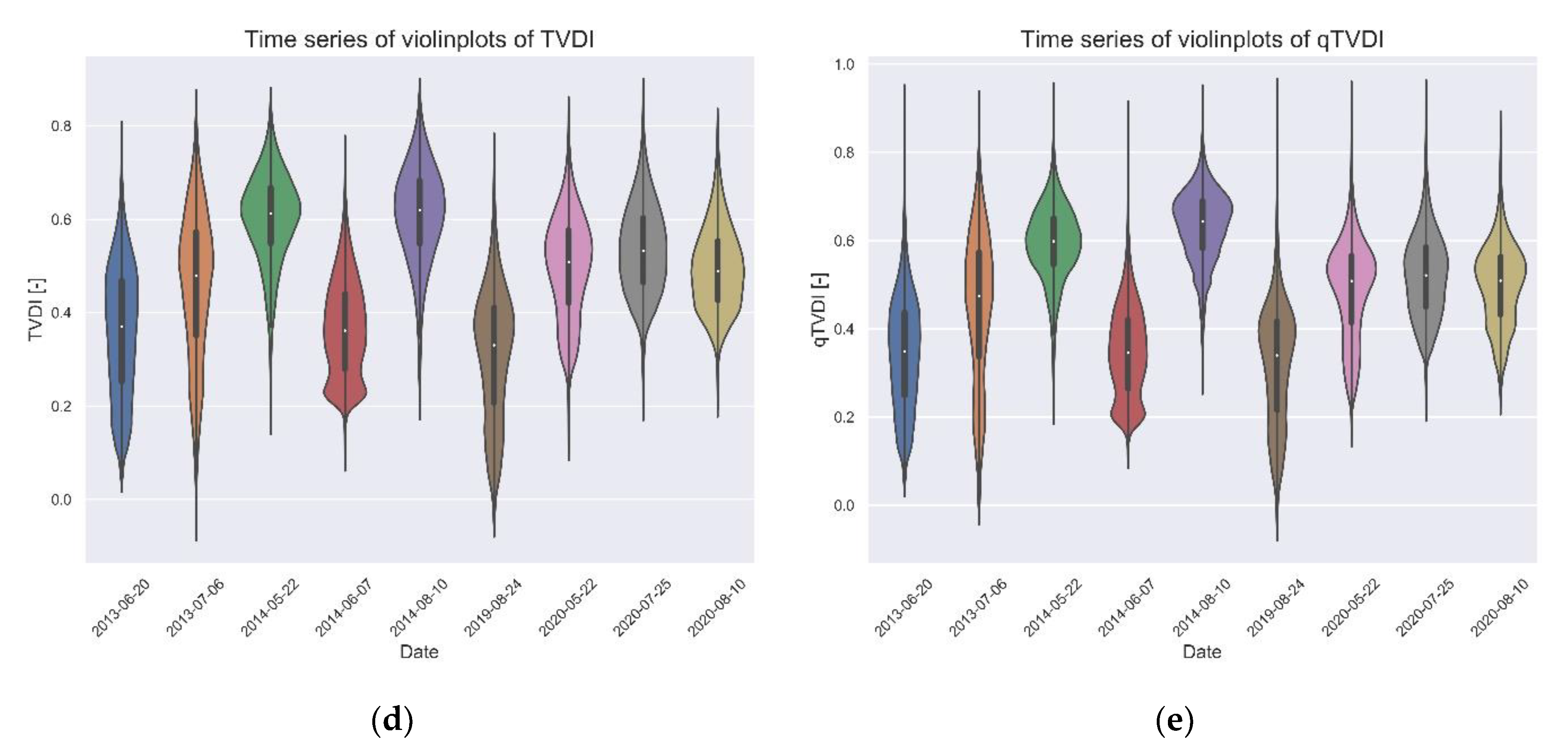
Figure 2a–e shows how the statistical distribution of the analyzed parameters changes over time for the entire city.

Moreover, Figure 2 shows how each of the analyzed parameters changes over time for the whole city. LST varies for all dates, and there is no apparent trend. This is mainly due to the fact that the analyzed images are taken from different months, and the only requirement was that they should be taken from the beginning of May to the end of August. In the case of NDBI, TVDI, and qTVDI, there is also only a minor positive trend, which may be related to rapidly advancing city development and building density. Additionally, the NDVI trend is negative, suggesting that the overall vegetation condition in Warsaw is gradually decreasing.

However, attention should be paid to the shape of the statistical distributions of the examined parameters. In the case of LST, these are left-skewed distributions in all cases, which means that most pixels have a temperature lower than the mean value. Observing the LST distributions, it can be seen that large differences between the lowest and highest temperatures are noticeable, which in extreme cases even exceed 20 degrees Celsius. Temperature differences in the typical ranges of variation, i.e., between the third and second quartiles, are much smaller and usually amount to around 5 degrees Celsius. The above observations prove that the areas of increased temperature concern densely built-up parts of the city, of which there is a minority in Warsaw. Interestingly, the NDBI distributions are also similar to NDVI ones, which confirms that the extreme temperatures result from the heating of built-up areas. The NDVI distributions, on the other hand, have a left-skewed distribution, which means that significant parts of the city are covered with vegetation. Likewise, most TVDI and qTVDI distributions are also left-skewed, meaning that most of the city’s surface has relatively dry soils.

4.3. Correlation of Estimated Parameters for the Whole Research Area

The authors calculated Pearson’s correlation coefficient matrix between the analyzed indexes for each studied satellite image of the entire area of Warsaw. The correlation coefficients between LST and NDBI, TVDI, and qTVDI are positive, whereas the ones between LST and NDVI are negative.

Table 4. Pearson’s correlation coefficients between the analyzed indexes calculated for the entire area of Warsaw for 8 August 2020.

	LST	NDBI	NDVI	TVDI	qTVDI
LST	1.00	0.83	−0.86	0.34	0.78
NDBI		1.00	−0.88	−0.02	0.45
NDVI			1.00	0.19	−0.37
TVDI				1.00	0.83
qTVDI					1.00

presents exemplary Pearson’s correlation coefficients calculated for 8 August 2020. The results for other dates are similar and can be found in the Supplementary Materials (Table S1).

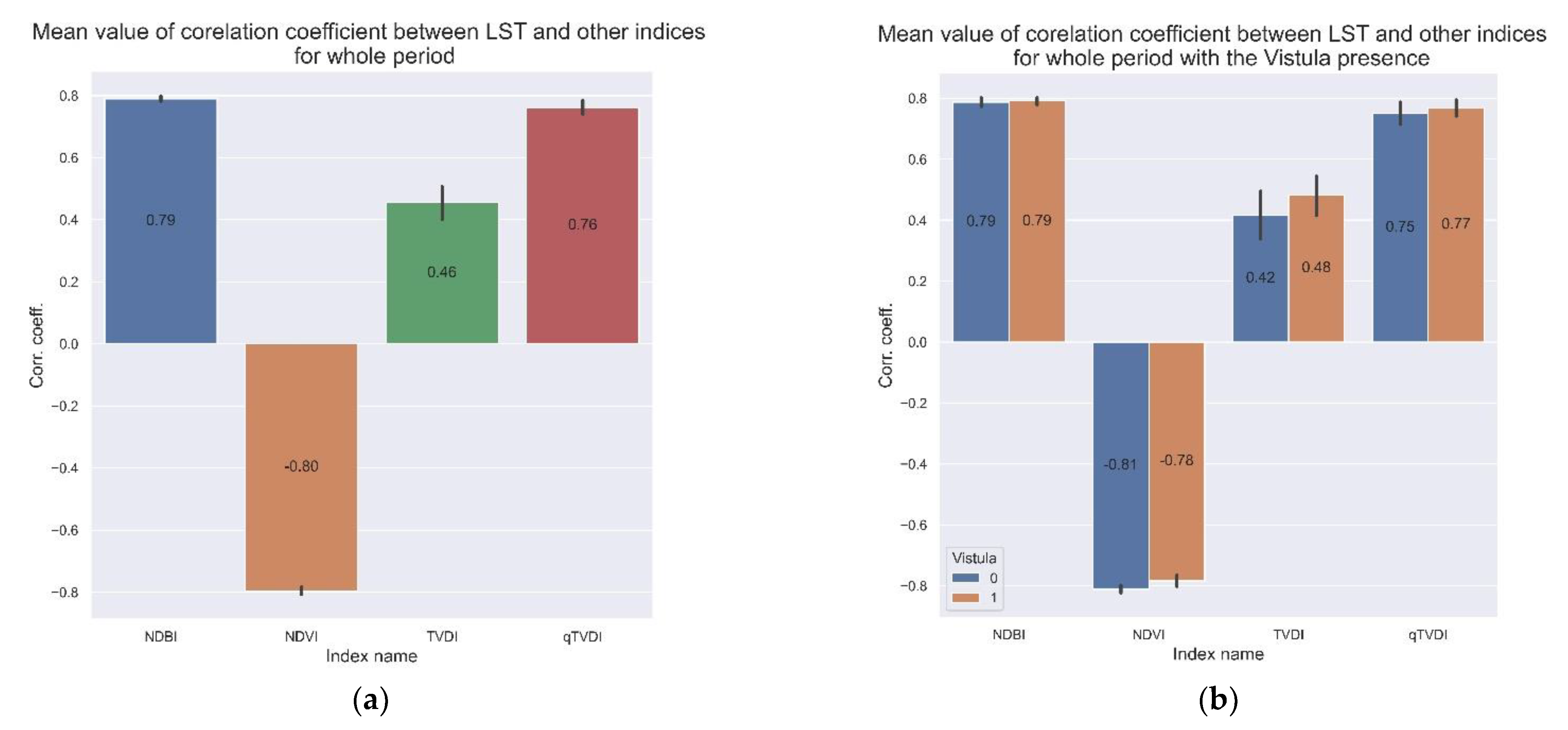
In Figure 3a,b, the mean values of the correlation coefficients between LST and other indexes calculated for each date are shown in the form of bar plots. The values of indexes taken for the mean calculations shown in Figure 3a are calculated from the entire Warsaw area, whereas in Figure 3b, the calculated mean values were calculated separately from the districts having access to the Vistula River (blue color) or not (orange color).

The highest values of correlation coefficient modulus are observed for NDVI, NBDI, and qTVDI, and all are close to 0.8, which is very high. Thus, those parameters best reflect phenomena that are responsible for urban heat island development (NBDI and qTVDI—the positive values of correlation coefficients) or mitigation (NDVI—the negative values of correlation coefficients). As described above, in Table 4, the mean values of Pearson’s correlation coefficients between LST and other indexes calculated for districts with or without access to the Vistula River are shown. As expected, the correlation coefficients between LST and NBDI are similar in coastal districts and those without access to the Vistula coast. The reason for such a result may be that the area of the river in relation to the undeveloped area of the big agglomeration is too small to cause visible changes in the correlation coefficient. Visible, but still minor, differences in the studied correlation coefficients between coastal and noncoastal ones are found for TVDI/qTVDI and NDVI. It should be remembered, however, that the Vistula River is the border of Warsaw’s districts and does not flow through them.

4.4. Crosswise Distribution of the Studied Parameters and the Dependence of LST on Them in Terms of Districts and Dates

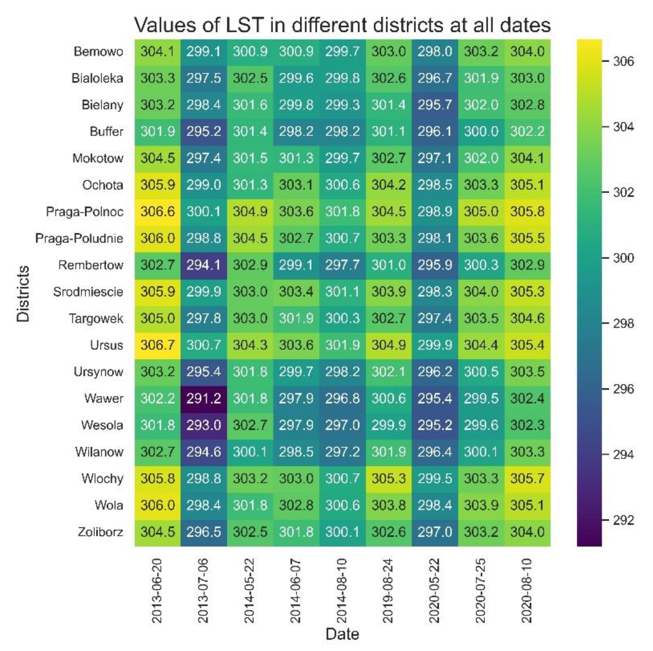
In this section, the authors present the distributions of mean values of LST, NDVI, TVDI, qTDVI, and NDBI, as well as correlation coefficients between LST and other parameters, across all districts and studied dates. Figure 4a shows the distribution of the mean values of LST across districts and dates.

As discussed above in Section 4.3 (Figure 3b), the influence of the Vistula River on the LST was surprisingly small. Therefore, to study this phenomenon in detail, it was decided to first compare the LST distribution (across districts and dates) (Figure 5a) with the analogous distribution of the percentage of pixels classified as water and mean temperature (Figure 5b).

The juxtaposition also shows no apparent correlation between the percentage of pixels classified as water and the mean temperature on the scale of Warsaw districts. This may be because half of the riverside districts that have the biggest percentage of water pixels are also located in the densely built-up city center (Środmieście, Żoliborz, Praga-Polnoc, Praga Poludnie districts). It can therefore be concluded that the presence of built-up areas (NDBI) and vegetation (NDVI) has a large influence on the surface temperature in Warsaw (LST).

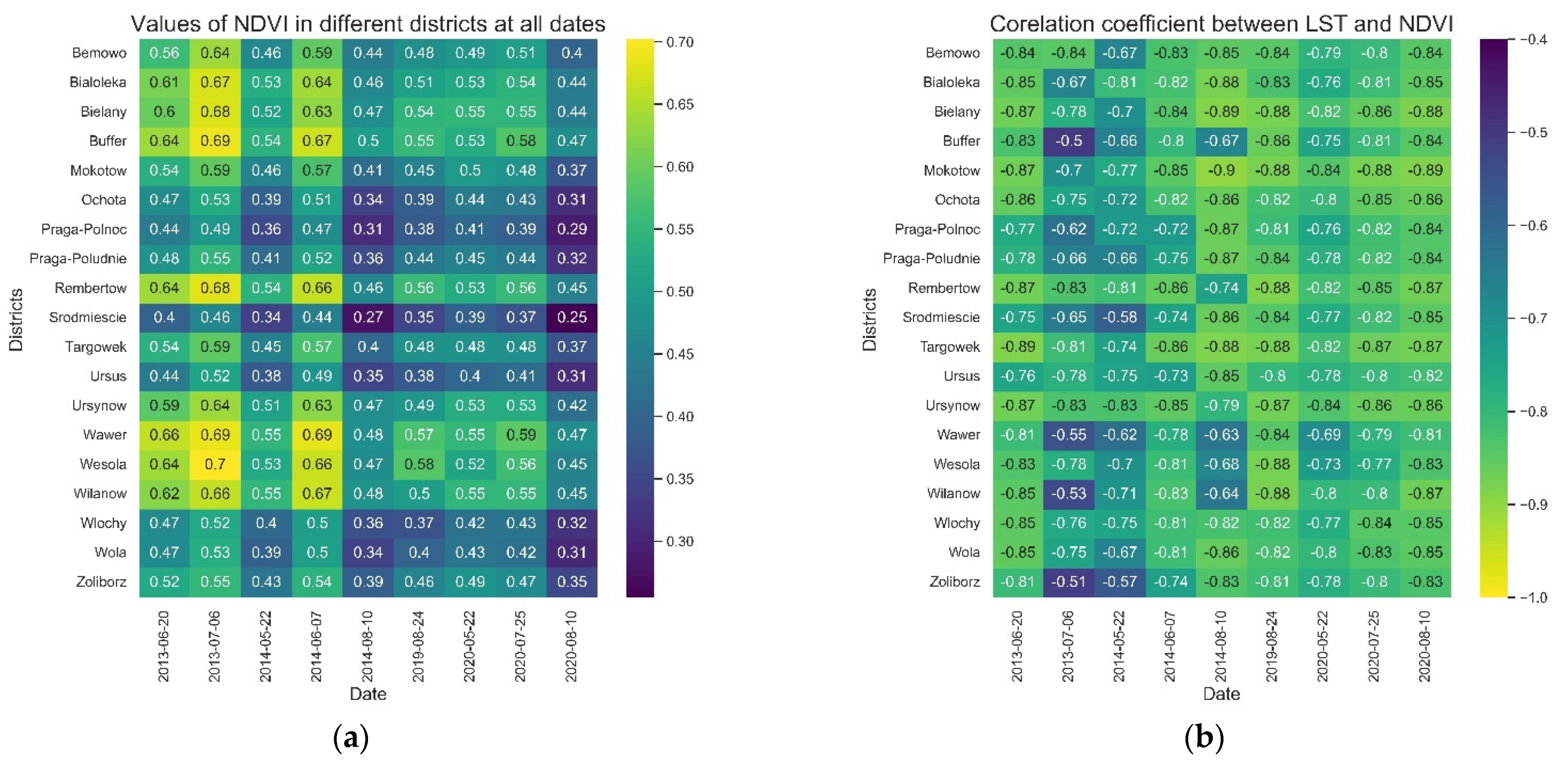
Figure 5 shows the distributions of mean values of NDVI, NDBI, TVDI, and qTDVI as well as correlation coefficients between LST and these parameters across all districts and studied dates.

Analyzing information in Figure 5a–d, it can be seen that districts that have higher values of NDVI and lower values of NDBI (Rembertów, Ursynów, Wawer, Wesoła, Wilanów) have, in general, lower mean temperatures.

It should be emphasized that, in general, the correlation coefficients between LST and NDVI and NDBI have very high values, which are negative for NDVI and positive for NDBI. This proves a very large influence of urban vegetation and buildings on the temperature distribution in the city districts. This is an important result, as it allows the general relationships between LST and NDVI and NDBI to be disaggregated to the scale of individual districts where decisions regarding spatial management are made.

Comparing Figure 5f,h, it is clear that the improved qTVDI index gives clearly better results than the classic TVDI, as it can be expected that higher temperature is correlated with a lower soil moisture level, i.e., a higher average TVDI/qTVDI value.

The correlation coefficients between mean LST temperatures and mean qTVDI values are comparable (in absolute value) to those between LST and NDVI, or LST and NDBI (see Figure 3a, and Figure 5b,d,h). Additionally, it can be concluded that soil moisture in a large area of the city has a much greater impact on temperature than even the relatively large main stream of the Vistula River, which, however, has a small area compared to the city’s area.

The buffer, which is 5000 m in width, from the Warsaw administrative borders has one of the highest mean values of NDVI and the lowest mean values of NDBI and qTVDI, which is expected, due to the large distance from the densely built city center. However, there is no striking difference between the studied parameters in the buffer and those of districts located on the outskirts of the city such as Białołęka, Bielany, Wawer, Ursynów, Włochy, etc. These districts also have a lot of green areas and little compact development, and they do not differ much from the suburban areas with many smaller towns. More distinct differences between unfavorable urban climate changes occur within the city and between particular districts because, depending on their character and function, there are larger differences in the type of development.

5. Conclusions

In the presented research, the correlations between vegetation, built-up (impervious) areas, soil moisture, and land surface temperature in the capital city of Warsaw were analyzed using satellite-derived indexes. The study area of this research was the entire city of Warsaw as well as 18 individual districts and the closest suburbs. The obtained results confirmed that building density significantly increases the surface temperature in the city, while the presence of urban vegetation significantly lowers it. The influence of the Vistula River on lowering the temperature, due to the large size of the city, turned out to be rather local and smaller than initially expected. On the other hand, an unexpectedly important factor influencing the temperature of the Earth’s surface turned out to be soil moisture, the cooling effect of which affects the entire studied area of the city, the nearest suburbs, and individual districts. The impact of soil moisture on LST can be compared in size to the effect of vegetation, or, in absolute values, to the ratio of built-up area, determined by the NDBI index. Thus, the work presents important practical conclusions, e.g., that impermeable surfaces not only increase the possibility of city flooding but also contribute to a significant increase in surface temperature. This kind of analysis is relevant to planners/policy makers in cities who seek to better understand the spatial variability of Land Surface Temperature and its relations with green areas and impervious areas [36]. The quantitative results obtained in the article on the influence of soil moisture on city temperature could allow urban planners/policy makers of Warsaw to design urban design much better in order to improve the thermal comfort of inhabitants. Another important result of the work is also that it shows that the differences in the analyzed indicators may be greater between individual districts than between districts from the outskirts of the city and suburban areas. In the future, it would be useful to perform a similar but more detailed analysis, on a smaller scale than that used in this paper, on the role of soil moisture in lowering the temperature in an urban agglomeration. We would also like to emphasize that great caution is needed in interpreting the soil moisture in urban areas calculated using the triangle method, due, among other reasons, to the existence of impervious surfaces that do not significantly retain water, which are usually surfaces such as a small fraction of bare soil or vegetated areas in cities, shaded areas, etc. All these factors should be taken into account in future models of soil moisture in urban areas.

Procedures used to carry out the research, especially those which could calculate investigated indexes, were based on Python 3 and open source libraries and are published together with the article. Data used for those analyses are also available in [30]. The necessary data are Landsat 8 OLI/TIRS images, which could also be obtained free of charge, i.e., from Earth Explorer [30], and vector files of the region of interest.

References

1. United Nations. World Population Prospects, the 2019 Revision-Volume I: Comprehensive Tables; United Nations: New York, NY, USA, 2019; ISBN 978-92-1-004642-8.
2. Mensah, C.A. Destruction of Urban Green Spaces: A Problem Beyond Urbanization in Kumasi City (Ghana). Am. J. Environ. Prot. 2014, 3, 1. [Google Scholar] [CrossRef] [Green Version]
3. Moreno, R.; Ojeda, N.; Azócar, J.; Venegas, C.; Inostroza, L. Application of NDVI for Identify Potentiality of the Urban Forest for the Design of a Green Corridors System in Intermediary Cities of Latin America: Case Study, Temuco, Chile. Urban For. Urban Green. 2020, 55, 126821. [Google Scholar] [CrossRef]
4. Gawuc, L.; Jefimow, M.; Szymankiewicz, K.; Kuchcik, M.; Sattari, A.; Struzewska, J. Statistical Modeling of Urban Heat Island Intensity in Warsaw, Poland Using Simultaneous Air and Surface Temperature Observations. IEEE J. Sel. Top. Appl. Earth Obs. Remote Sens. 2020, 13, 2716–2728. [Google Scholar] [CrossRef]
5. Mora, C.; Dousset, B.; Caldwell, I.R.; Powell, F.E.; Geronimo, R.C.; Bielecki, C.R.; Counsell, C.W.W.; Dietrich, B.S.; Johnston, E.T.; Louis, L.V.; et al. Global Risk of Deadly Heat. Nat. Clim. Chang. 2017, 7, 501–506. [Google Scholar] [CrossRef] [Green Version]
6. Venter, Z.S.; Brousse, O.; Esau, I.; Meier, F. Hyperlocal Mapping of Urban Air Temperature Using Remote Sensing and Crowdsourced Weather Data. Remote Sens. Environ. 2020, 242, 111791. [Google Scholar] [CrossRef]
7. Bizjak, M.; Žalik, B.; Štumberger, G.; Lukač, N. Estimation and Optimisation of Buildings’ Thermal Load Using LiDAR Data. Build. Environ. 2018, 128, 12–21. [Google Scholar] [CrossRef]
8. Van, T.T.; Tran, N.D.H.; Bao, H.D.X.; Phuong, D.T.T.; Hoa, P.K.; Han, T.T.N. Optical Remote Sensing Method for Detecting Urban Green Space as Indicator Serving City Sustainable Development. Proceedings 2017, 2, 140. [Google Scholar] [CrossRef] [Green Version]
9. Haq, S.M.A. Urban Green Spaces and an Integrative Approach to Sustainable Environment. J. Environ. Prot. 2011, 02, 601–608. [Google Scholar] [CrossRef] [Green Version]
10. Liu, Y.; Meng, Q.; Zhang, J.; Zhang, L.; Jancso, T.; Vatseva, R. An Effective Building Neighborhood Green Index Model for Measuring Urban Green Space. Int. J. Digit. Earth 2016, 9, 387–409. [Google Scholar] [CrossRef]
11. Hari, V.; Rakovec, O.; Markonis, Y.; Hanel, M.; Kumar, R. Increased Future Occurrences of the Exceptional 2018–2019 Central European Drought under Global Warming. Sci. Rep. 2020, 10, 12207. [Google Scholar] [CrossRef]
12. Zhang, R.; Zhao, C.; Ma, X.; Brindha, K.; Han, Q.; Li, C.; Zhao, X. Projected Spatiotemporal Dynamics of Drought under Global Warming in Central Asia. Sustainability 2019, 11, 4421. [Google Scholar] [CrossRef] [Green Version]
13. Vicente-Serrano, S.M.; Quiring, S.M.; Peña-Gallardo, M.; Yuan, S.; Domínguez-Castro, F. A Review of Environmental Droughts: Increased Risk under Global Warming? Earth-Sci. Rev. 2020, 201, 102953. [Google Scholar] [CrossRef]
14. Kong, D.; Gu, X.; Li, J.; Ren, G.; Liu, J. Contributions of Global Warming and Urbanization to the Intensification of Human-Perceived Heatwaves Over China. J. Geophys. Res. Atmospheres 2020, 125, e2019JD032175. [Google Scholar] [CrossRef]
15. Lemonsu, A.; Viguié, V.; Daniel, M.; Masson, V. Vulnerability to Heat Waves: Impact of Urban Expansion Scenarios on Urban Heat Island and Heat Stress in Paris (France). Urban Clim. 2015, 14, 586–605. [Google Scholar] [CrossRef]
16. Mariani, L.; Parisi, S.G.; Cola, G.; Lafortezza, R.; Colangelo, G.; Sanesi, G. Climatological Analysis of the Mitigating Effect of Vegetation on the Urban Heat Island of Milan, Italy. Sci. Total Environ. 2016, 569–570, 762–773. [Google Scholar] [CrossRef]
17. Qiu, G.; Li, H.; Zhang, Q.; Chen, W.; Liang, X.; Li, X. Effects of Evapotranspiration on Mitigation of Urban Temperature by Vegetation and Urban Agriculture. J. Integr. Agric. 2013, 12, 1307–1315. [Google Scholar] [CrossRef]
18. Chun, B.; Guldmann, J.-M. Impact of Greening on the Urban Heat Island: Seasonal Variations and Mitigation Strategies. Comput. Environ. Urban Syst. 2018, 71, 165–176. [Google Scholar] [CrossRef]
19. Sandholt, I.; Rasmussen, K.; Andersen, J. A Simple Interpretation of the Surface Temperature/Vegetation Index Space for Assessment of Surface Moisture Status. Remote Sens. Environ. 2002, 79, 213–224. [Google Scholar] [CrossRef]
20. Gillies, R.R.; Kustas, W.P.; Humes, K.S. A Verification of the “triangle” Method for Obtaining Surface Soil Water Content and Energy Fluxes from Remote Measurements of the Normalized Difference Vegetation Index (NDVI) and Surface e. Int. J. Remote Sens. 1997, 18, 3145–3166. [Google Scholar] [CrossRef]
21. Wang, C.; Qi, S.; Niu, Z.; Wang, J. Evaluating Soil Moisture Status in China Using the Temperature–Vegetation Dryness Index (TVDI). Can. J. Remote Sens. 2004, 30, 671–679. [Google Scholar] [CrossRef]
22. Carlson, T. An Overview of the “Triangle Method” for Estimating Surface Evapotranspiration and Soil Moisture from Satellite Imagery. Sensors 2007, 7, 1612–1629. [Google Scholar] [CrossRef] [Green Version]
23. Petropoulos, G.P.; Ireland, G.; Barrett, B. Surface Soil Moisture Retrievals from Remote Sensing: Current Status, Products & Future Trends. Phys. Chem. Earth Parts ABC 2015, 83–84, 36–56. [Google Scholar] [CrossRef]
24. Przeździecki, K.; Zawadzki, J.J. Triangle Method Modification with Second Degree Polynomial Edges Fitting in LST NDVI Scatterplot in Lignite Mine Influence Area. Remote Sens. Appl. Soc. Environ. 2020, 20, 100404. [Google Scholar] [CrossRef]
25. Köppen Climate Classification (Weatherbase). Available online: http://www.weatherbase.com/weather/weather-summary.php3?s=57321&cityname=Warsaw,+Poland (accessed on 25 February 2022).
26. Lindner-Cendrowska, K.; Błażejczyk, K. Impact of Selected Personal Factors on Seasonal Variability of Recreationist Weather Perceptions and Preferences in Warsaw (Poland). Int. J. Biometeorol. 2018, 62, 113–125. [Google Scholar] [CrossRef] [PubMed] [Green Version]
27. Urząd Statystyczny w Warszawie/Dane o Województwie/Stolica Województwa/Ludność. Available online: https://warszawa.stat.gov.pl/dane-o-wojewodztwie/stolica-wojewodztwa/ludnosc/ (accessed on 25 February 2022).
28. EROS Landsat 8 (L8) Data Users Handbook; U.S. Geological Survey: Sioux Falls, SD, USA, 2019; p. 114.
29. Landsat Levels of Processing. Available online: https://www.usgs.gov/land-resources/nli/landsat/landsat-levels-processing (accessed on 8 April 2020).
30. EarthExplorer. Available online: https://earthexplorer.usgs.gov/ (accessed on 19 March 2022).
31. Chavez, P. Image-Based Atmospheric Corrections-Revisited and Improved. Photogramm. Eng. Remote Sens. 1996, 62, 1025–1035. [Google Scholar]
32. Xu, H. Modification of Normalised Difference Water Index (NDWI) to Enhance Open Water Features in Remotely Sensed Imagery. Int. J. Remote Sens. 2006, 27, 3025–3033. [Google Scholar] [CrossRef]
33. Bhatti, S.S.; Tripathi, N.K. Built-up Area Extraction Using Landsat 8 OLI Imagery. GIScience Remote Sens. 2014, 51, 445–467. [Google Scholar] [CrossRef] [Green Version]
34. Zawadzki, J.; Przeździecki, K.; Miatkowski, Z. Determining the Area of Influence of Depression Cone in the Vicinity of Lignite Mine by Means of Triangle Method and LANDSAT TM/ETM+ Satellite Images. J. Environ. Manage. 2016, 166, 605–614. [Google Scholar] [CrossRef]
35. Zha, Y.; Gao, J.; Ni, S. Use of Normalized Difference Built-up Index in Automatically Mapping Urban Areas from TM Imagery. Int. J. Remote Sens. 2003, 24, 583–594. [Google Scholar] [CrossRef]
36. Wetherley, E.B.; McFadden, J.P.; Roberts, D.A. Megacity-Scale Analysis of Urban Vegetation Temperatures. Remote Sens. Environ. 2018, 213, 18–33. [Google Scholar] [CrossRef]
Figure 1. Research area with Warsaw administrative border and division into districts.
Sustainability 15 01274 g001
Figure 2. Violin plots of analyzed indexes which show the distributions of the studied indexes for all of the studied dates. White dots on the violin plot denote medians, and interquartile ranges (IQRs) are shown by thick black bars. The black lines stretched from the bars denote the range of the values first quartile minus 1.5 IQR and third quartile plus 1.5 IQR.
Sustainability 15 01274 g002aSustainability 15 01274 g002b
Figure 3. The mean values of Pearson’s correlation coefficients between LST and other indexes calculated for all dates and the entire Warsaw area (a) or with the division into districts through which the Vistula River flows ((b), blue color) or not ((b), orange color).
Sustainability 15 01274 g003
Figure 4. Heatmaps of LST mean values in districts at all dates. The temperature in the legend is given in Kelvin.
Sustainability 15 01274 g004
Figure 5. Heatmaps of indexes’ mean values in districts at all dates (left) and correlation coefficients between those indexes and LST (right). (a,c,e,g) the values of NDVI, NDBI, TVDI, and qTVDI in different districts at all dates, respectively. (b,d,f,h) Pearson’s correlation coefficients between LST and NDVI, NDBI, TVDI, as well as qTVDI in different districts at all dates, respectively.
Sustainability 15 01274 g005aSustainability 15 01274 g005b