Abstract
With the recent climate changes, investors and policy-makers are paying close attention to the green bond market. This study intends to analyze the dynamic effects of shock transmission between climate policy uncertainty and the green bond market and to offer some new perspectives on analysis of green bond volatility over the previous years. To investigate time-varying effects of climate policy uncertainty on green bond market volatility, we applied a TVP-VAR model. And the impact of three important time points is tested, which are the Paris Association convening in December 2015, the 2017 annual Report on Policies and Actions of China on Climate Change in October 2017 and the “double carbon” policy in September 2020. The finding is that: (1) This impact of climate policy uncertainty on the volatility of the green bond market is time-varying, with short-term overreactions or underreactions as well as medium and long-term inversions. (2) This impact is also time-varying at different time points and has a certain degree of sustainability.
1. Introduction
We investigated the effect of climate policy uncertainty on green bond market volatility at the level of time-series. Global climate change and socially responsible investment behavior have become important topics in academia (see Liu [1], Tian et al. [2]). As the global warming trend becomes increasingly severe, output and labor productivity may be severely affected [3]. Moreover, as climate change mitigation policies are implemented one after another, prices, productivity, employment, and output will all be affected, and monetary policy is no exception. Thus, the great uncertainty of climate-related events and policies may dampen investment and other economic activities. In the event of extreme weather conditions such as heavy rainstorms, the government may introduce relevant climate policies, and with climate policies constantly being adjusted, the impact of climate-related policies on the green bond market cannot be ignored, considering the purpose of green bond creation. Further, the formulation, implementation, and adjustment of climate policies are influenced by the objective natural environment, human awareness, and emergencies, and it is difficult to predict the possibility of future climate events when climate policies change. Because of the “bond” nature of green bonds, the impact of monetary policies such as interest rates is also crucial, and monetary policy is also potentially influenced by climate policy. Therefore, this study explores the time-varying impact of climate policy uncertainty (CPU) on green bond market volatility.
CPU may affect financial markets [4,5], so does CPU increase green bond price volatility and exacerbate the risk in the market? As a debt asset, changes in the green bond price will also be more influenced by market behavior, such as changes in interest rates and investor sentiment. Therefore, in the short term, green bond price volatility is more likely to be noticed by investors due to the impact of CPU by investors and may trigger an overreaction; however, considering the impact of investor sentiment, a high level of investor sentiment and a weakened perception of risk in a bull market may also trigger an underreaction. At the same time, as climate policy changes will affect monetary policy, for example, changes in interest rates will also inevitably affect green bond price volatility, and investor sentiment toward green bond price volatility can also change during periods of easing or tightening interest rates, leading to an overreaction or underreaction to green bond market risk. In the medium and long term, if the increasing severity of climate problems and the introduction and adjustment of climate policies are generally supportive of green development, then the long-term implications of green bond market price volatility from CPU are likely to be negative. Combining these characteristics, for the lower trading rate in the green bond market, more information may be accumulated in pricing to be released in the next transaction, and the price volatility at the time of trading may be greater.
Green bonds are sustainable debt instruments created to mitigate climate problems, and as an important emerging financial market, the green bond market has shown characteristics of “a bull market is more bullish and a bear market is more bearish”, and its volatility-related studies have begun to receive academic attention [1,6,7].Therefore, to clarify whether CPU affects the volatility of the green bond market and whether the impact has a dynamic effect, this paper adopted the TVP-VAR model to investigate, and its academic contributions are as follows: First, it demonstrates theoretical analysis of what climate policy uncertainty affects volatility of the green bond market, which provides theoretical support for regulators to respond to climate policy adjustments, thus promoting green bond market supervision and management. Second, it is the first empirical study of how CPU affects the price volatility of green bonds in China, enriching the scope of research on climate finance and providing an important basis for investors in green bonds to make risk management decisions and regulators to respond to climate risks.
The remainder of this study is structured as follows: Section 2 reviews the institutional background in China; Section 3 reviews the relevant literature; Section 4 describes the research design, including method and data; Section 5 is empirical results and discussion, and finally, some results are summarized.
2. Background in China
With the frequent occurrence of extreme weather and severe environmental problems, China has reshaped its development philosophy, continuously promoted a comprehensive green transformation of the economy and society, and strived to build a beautiful China where people and nature coexist in harmony. As shown in Figure 1, China has introduced numerous climate policies to mitigate climate problems in recent years, and President Xi proposed for the first time that China should achieve “peak carbon” by 2030 and “carbon neutral” by 2060 in September 2020. This is an important step in the process of transition to a low-carbon economy in China. Green development is inseparable from financial support; in addition to government financial support and enterprise self-financing, green bonds are an important funding channel.
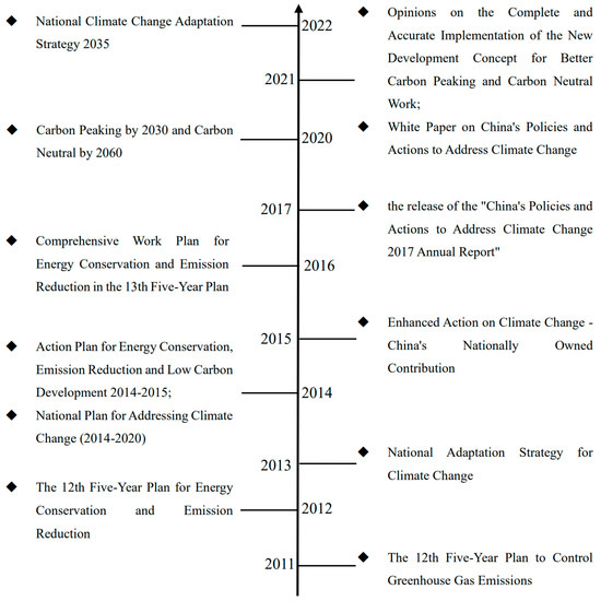
Figure 1.
Overview of China’s climate policy (2011–2022).
The General Plan for the Reform of Ecological Civilization System and the Catalogue of Green Bond Support Projects (2015 Edition) defined the classification criteria of green bonds for the first time. As shown in Figure 2, since the Chinese green bond market began to boom in 2016, China’s labeled green bond issuance has increased rapidly, and although there may have been a brief pullback in 2020 due to the epidemic and other impacts, China’s total green bond issuance in 2021 bucked the trend by 140%, achieving the largest annual increment to nearly USD 110 billion. As the projects supported by green bonds generally have longer maturities, their maturities tend to be longer than ordinary bonds as well. The credit ratings of green bonds are also generally concentrated in high ratings. It can be seen that its activity level is low. In July 2022, the document “China Green Bond Principles” was released, which became the first policy document stipulating uniform standards for green bond issuance. With the introduction of various guiding policies, the green bond market has flourished and increased rapidly in size.
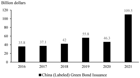
Figure 2.
Annual issuance in China’s green bond market. Data come from the annual “Green Bond Market Report” and manually compiled by authors.
The booming development of the green bond market is evident worldwide. As shown in Figure 3, according to a related report released by the Climate Bonds Initiative in 2021, the cumulative issue volume of China’s green bonds was the second in the world, which also fully illustrates the importance of China’s green bond market in the global green bond market. As a result, research on the green bond market has also been pursued by a number of scholars.
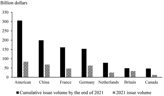
Figure 3.
Green Bond Issuance by Major Countries in the World in 2021. Source from “China Green Bond Market Report 2021”.
3. Literature Review
The green bond market has emerged as an important part of China’s capital market, and more and more scholars are focusing on its development and growth. Studies about green bond pricing [8,9,10,11], the impact on issuing firms [9,12,13], and the connection between the green bond market and other financial markets [14,15,16,17], among others, have been emerging, contributing to an in-depth understanding of the operation of the green bond market and providing theoretical support for its supervision and guidance. Meanwhile, the risk of the green bond market is a very important topic that has received much attention from scholars and the practical community.
3.1. Green Bond Market
Several scholars have enriched the risk of green bonds from the perspectives of credit spreads and risk premiums. Wang et al. [18] studied the influence of macro and micro factors on the green bond risk premium in China and found that third-party certification, ratings, etc., tend to reduce green bond yield, thus reducing the financing cost of issuers. Zerbib [11] found a negative green premium of 2 basis points between the yield spread of green bonds and matching conventional bonds through a matching method study. Tang and Zhang [9] had a negative premium of 6.94 basis points in the green bond market for the full sample, but not when issuer characteristics were considered. Later, MacAskill et al. [19] found that a green premium exists in 56% of primary market studies and 70% of secondary market studies by summarizing the relevant green premium research literature.
Some scholars have also studied the risk through its volatility from the viewpoint of the green bond market. Pham [6] first discovered that green bond volatility is characterized by volatility clustering, heteroskedasticity, and non-normal distribution. Pham and Huynh [7] found that green bond volatility is affected by investor attention over time. Subsequently, Xia et al. [20] proposed two novel heteroskedasticity integration models to predict green bond market volatility. In the meantime, Liu [1] examined how COVID-19 affected green bond volatility and indicated significant volatility as well as significant negative abnormal returns in the green bond under the epidemic shock. Relatively few studies have examined green bond market risk from a volatility standpoint.
In fact, quite a few scholars analyze the market price risk of green bonds by studying the correlation between the green bond market and other financial and commodity markets. Reboredo [15] pointed out that the green bond market is highly correlated with the bond market and the money market, but has a weak link with the stock and energy markets [16]. In addition, some scholars have found that green bonds are negatively correlated with WTI and Brent crude oil prices [21], and there is also a negative correlation with carbon futures returns [14]. Since 2020, affected by COVID-19, the asset market has fluctuated dramatically. Many scholars have begun to study the risk spillover effect between green bonds and different assets based on this background. For example, Naeem et al. [22] examined the risk spillover effects of green bonds and stocks and bonds based on quantitative methods. He believed that green bonds have a substitution effect with traditional bonds, and in low-risk periods, green bonds can provide diversified investment. Tiwari et al. [23] used the TVP-VAR method to study the asset price pass-through effect of green bonds and clean energy stocks, and found that the linkage between asset prices is heterogeneous and changes over time and that green bonds are often the recipients of other asset price shocks [24].
3.2. Climate Change and Financial Markets
Climate risk, as a new type of macroeconomic risk, is also of interest to scholars in terms of its impact on financial markets. The complexity of the climate system makes the metrics of climate risk not yet uniform, and most scholars measure climate risk by using data such as temperature and drought [3,25,26]. In recent years, scholars have studied the relationship between climate risk and financial markets from different perspectives. Painter [27] found that initial yields and underwritten costs were higher for long-term local government bonds related to climate change. Seltzer et al. [28] empirically analyzed and found that climate transition risk affects the risk assessment and pricing of corporate bonds. Huynh and Xia [29] found that corporate bonds that are positively correlated with the climate news index have lower yields. Given the difficulty of predicting climate risk and the frequent and unpredictable adjustment of related policies, the risks induced by CPU in the capital market are gaining attention. Barnett et al. [30] argued that CPU will lead to changes in investor subjective discount rates in response to climate change. Barro [31] argued that optimal environmental investment increases as the effectiveness of the CPU increases and decreases. Bouri et al. [4] found that CPU has a more significant impact on green energy stocks compared to brown energy stocks and that the effect of CPU on green energy stocks is positive.
The main elements of earlier literaturesliterature are summarized in Table 1. Overall, the impact of CPU on financial markets cannot be ignored. Academics have also begun to extensively study the impact of climate policy changes on financial markets. Adjustments to climate policy changes are systematic and uncertain, and can significantly affect asset prices in equity and bond markets, but there is little literature on how climate policy uncertainty affects green bond markets, especially the risk of green bond markets. Therefore, this study innovatively analyzes how climate policy uncertainty affects green bond price volatility to provide theoretical support for the stable and healthy development of the green bond market.

Table 1.
A summary of earlier studies.
4. Research Design
4.1. Methodology
From the previous analysis, it is clear that the impact of CPU on green bond volatility varies in different periods, so this study chooses the vector autoregressive (TVP-VAR) approach with time-varying parameters to study the time-varying impact of CPU on bond price volatility. The existing vector autoregressive (VAR) models are mainly used to predict and analyze the magnitude and direction of unconstrained stochastic perturbations on system shocks and their durations. Later, a large number of scholars successively proposed structural VAR (SVAR) models based on VAR models. SVAR models reduce the parameters to be estimated by adding constraints, which can alleviate the problem of dimensional catastrophe caused by VAR models when there are too many objects under study. Primiceri [32] introduced the characteristics of time-varying parameters into the SVAR model and proposed the TVP-SV-VAR model, which was introduced by Nakajima [33], who derived the construction process of the TVP-VAR model in detail on this basis and set the precondition of stochastic fluctuation of model variance to make it more consistent with the logic of economic operation. Since then, related scholars began to use the model to conduct empirical studies on macroeconomic issues [34,35].
Before building the TVP-VAR model, a VAR model needs to be constructed, which has the basic form of
Among them, the is the dimensional time series observation column vectors, the are dimensional parameter matrix, and the perturbation term are dimensional structural shock column vector, assuming , where
Based on the recursive identification of synchronization relations in structural shocks, the lower triangular matrix can be obtained:
Thus, by transferring the matrix to the other side of the equation, the SVAR model can be obtained in short form as follows:
where , the is a dimensional column vector, obtained by obtained by superimposing all the row elements in Define , where denotes the Kronecker product, which gives a more simplified form of the model as:
If all the parameters in the above assumptions are made to be able to change with time, then we can obtain:
Equation (4) above is the basic form of the TVP-VAR model, where the coefficients , the joint parameter matrix and the covariance matrix of the stochastic fluctuations are time-varying. According to Primiceri [32], Nakajima [33], and Vuong et al. [36], the definition , , where . Similarly, we assume that the parameters in (4) follow the following random wandering process:
where, .
According to the algorithm of Nakajima [33], this study uses MCMC sampling method to estimate the model, such that , set be the the prior probability density. For the given data , the posterior distribution of is sampled.
4.2. Variables
Climate policy uncertainty indicator. Climate Policy Uncertainty refers to the difficulty in predicting the likelihood of future climate events when climate policy changes. Gavriilidis [37] constructed a CPU index with the help of big data methods based on keywords such as “uncertainty”, “environment”, “climate change”, “climate risk”, “policy”, “legal”, and “regulatory”. Figure 4 shows the CPU annotated index, which includes the U.S–China Joint Statement on Climate Change, the UN Climate Action Summit (China’s position and actions), etc. It contains many international climate policy changes, and China has been actively cooperating with the global community to address climate change in the past decade, and Ren et al. [38] used this index to study total factor productivity in China. For this reason, this index was selected to measure climate policy uncertainty (CPU) and examine its impact on green bond price volatility.
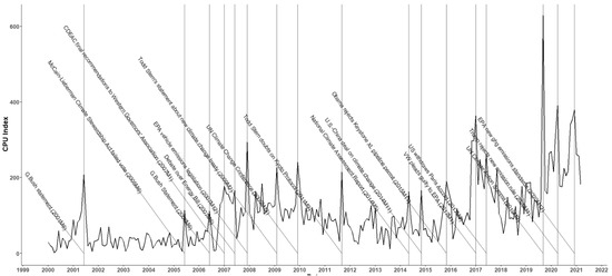
Figure 4.
CPU index.
Green Bond Index. This study selected the China Bond Green Bond Index to measure the green bond market. The China Bond Green Bond Index is jointly compiled by the China Bond Financial Valuation Center and Hengyun Technology Services (Beijing) Co., Ltd. The constituent bonds of the index are mainly bonds that meet one of the criteria of the Green Bond Support Project Catalogue (2021 Edition), Green Bond Principles GBP 2021, and Climate Bond Standard. In addition, this study also selects the China Bond climate-related bond index as a proxy variable for robustness testing. The constituent bonds of the China Bond Climate Related Bond Index are bonds that mainly satisfy one of the criteria of the Green Bond Support Project Catalogue and the Climate Bond Classification Scheme.
Green bond volatility. For the calculation of volatility, this study refers to the method of Aye et al. [39] and Gkillas et al. [40] to calculate the volatility of green bonds for the current month by calculating their daily returns with the mathematical expression:
where is the volatility in month t, is the daily return on day i of month t, and denotes the number of trading days in month t.
4.3. Data
In this study, the sample interval was set from January 2010 to December 2021, which includes 12 years of monthly sample data, covering important climate policy-related events from the Paris Agreement meeting in 2015 to the recent introduction of China’s “double carbon” target. The two green bond price indices and the CPU index were obtained from the Wind and Economic Policy Uncertainty Index, respectively. In addition, this paper is a time series study, and the climate policy uncertainty index was logarithmically treated to prevent the pseudo-regression phenomenon due to non-stationary time series from affecting the accuracy of the empirical results and leading to errors in statistical inference.
The trends of the main variables are shown in Table 2 and Figure 5. Although the volatility of the China Bond Climate Bond Index is more dramatic, the volatility changes of the two indices are more synchronized, and the China Bond Climate Bond Index is more appropriate as a robustness test. CPU has been oscillating slightly over the sample period, which is consistent with the fact that China has continuously introduced policies to address climate change since 2015 (the “Double Carbon” target in September 2020, etc.). How climate policy uncertainty affects green bond price volatility is difficult to conclude from simple trend changes and needs to be further tested.
Table 2.
Descriptive statistics results.
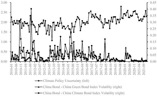
Figure 5.
Descriptive statistics of main indicators.
5. Empirical Results
The TVP-VAR model requires the variables to be smooth series, and the ADF test is used to determine their smoothness in this study. The test results of each variable are shown in Table 3. The ADF test statistics of all variables are significant at the 1% level, indicating that each variable is a smooth series and meets the model requirements.
Table 3.
Augmented Dickey–Fuller test.
It is also necessary to determine the optimal lag order before conducting empirical analysis with the TVP-VAR model. In this study, the information criterion was used to determine the number of lags, and the optimal lag order was not determined by the LL criterion, while lag 1 should be selected according to the SBIC criterion, and lag 2 should be selected according to the LR, FPE, AIC, and HQIC criteria. However, because the too-small lag order cannot guarantee that the random disturbance terms are white noise distributed, the lag period of the model was finally determined to be 2 periods in this study. The specific results are shown in Table 4.
Table 4.
Selection of model lags.
5.1. MCMC Simulation
For the parameters in the model, this study refers to the initial parameter settings of Nakajima [33] in the empirical study; After 10,000 simulations by the MCMC method, the first 1000 samples were discarded as aging values, and the posterior distribution of the parameters was estimated using the last 9000 samples. Figure 6, Figure 7 and Figure 8 and Table 5 report the estimation results for selected parameters of the TVP-VAR model for the variable set.
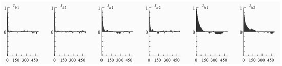
Figure 6.
Sample autocorrelation coefficient.
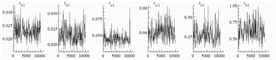
Figure 7.
Sample path.
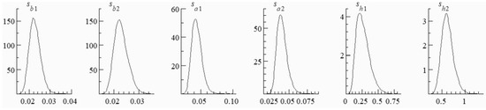
Figure 8.
Posterior densities.
Table 5.
Estimation results of selected parameters in the TVP-VAR model.
As shown in Figure 6, the autocorrelation coefficient of the sample shows a stable decreasing trend, which indicates that the sample data are smooth. The autocorrelation coefficient of parameter samples decreases gradually, and its fluctuation tends to zero after 500 times of MCMC. Figure 7 represents the smoothness of the sample fetching path, and it can be seen from Figure 7 that the sample path shows an overall up-and-down fluctuation with fewer extreme values, i.e., the sample fetching path is smooth. In addition, the graph in Figure 8 resembles posterior densities, indicating that the samples obtained by MCMC sampling with predefined parameters are valid. In addition, the inefficiency factors are quite low and the 95% confidence intervals include the estimated posterior mean for each of the parameters estimated. Therefore, the results show that posterior draws are efficiently produced by the MCMC algorithm.
Table 5 presents the estimation results computed using the MCMC algorithm, including the posterior means, standard deviation, and 95% credible intervals, Geweke convergence diagnostics statistics (Geweke), and inefficiency (Inef.). Among them, Geweke and the null factor are important for judging whether the MCMC sampling results are reasonable. Geweke is used to detect whether the sampling results of the model conform to the posterior distribution characteristics, while the null factor is the ratio of the variance of the posterior sample means to the variance of the uncorrelated serial sample means. The Geweke probabilities in Table 5 are significant at the 5% significance level (all Geweke values are less than 1.96), and all the inefficiency factors are less than 100, indicating that the sampled samples are valid for the posterior estimates of the TVP-VAR model.
5.2. Stochastic Volatility Estimation
Figure 9 reflects the stochastic volatility of CPU, GB and QH, from which it can be seen that there is a wave of a peak in CPU between 2013–2014, as well as a small peak in 2019–2020, which is to some extent also related to the intensity of relevant policies. The volatility of GB, on the other hand, is mainly reflected before 2012, which may also be related to the imperfect growth of the green bond market at this time.
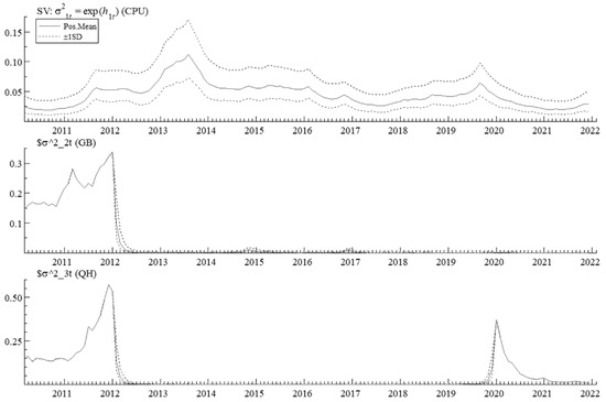
Figure 9.
Stochastic volatility of variable.
5.3. Time-Varying Impulse Response Estimation
The biggest advantage of the TVP-VAR model over the traditional VAR model is that the impulse responses of the variables can be estimated at various time points.
Figure 10 shows the simultaneous relation posterior estimates, and it indicates that the synchronization relationship of the structural shocks is time-varying. Figure 11 represents the time-varying impulse responses for a 0-month horizon, a 2-month horizon, and a 6-month horizon, respectively.
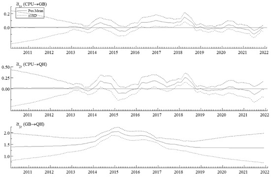
Figure 10.
Simultaneous relation posterior estimates.
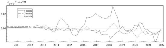
Figure 11.
Time-varying impulse response of CPU to GB.
Figure 11 shows the impulse response results of CPU on green bond price volatility. The impulse response function image oscillates up and down around the 0 point for the same time constraint and varies for different time constraints, indicating that the impact of CPU on green bond price volatility has a significant time-varying effect. This is mainly due to the fact that the domestic green bond market was not formally established at this stage, and the international green bond was also in its initial stage. By 2012, the green bond market was gradually recognized by various international financial organizations. From 2012 onwards, with the further development of the green bond market, CPU gradually shows a significant impact on the price volatility of the green bond market.
Between 2012 and mid-2015, the impact was mainly characterized by a small “up-down” process and reached its lowest point in mid-2015. This is mainly related to the development process of China’s green bond market. The period 2013–2014 saw rapid development of the international green bond market, with the growth rate of issuance remaining above 200%, which to a certain extent promoted the development of green bonds in China. At the same time, starting from the Eleventh Five-Year Plan, China began to formulate specific requirements for energy conservation and emission reduction in its development plan, and by the end of 2015, China’s green bond market was formally established. During this period, China continuously introduced various policies to address climate change, such as the incorporation of ecological civilization construction into the overall layout of the Five Branches of the Socialist Cause with Chinese Characteristics in the 18th Party Congress in May 2013. Green development has received wide attention and importance, such as the introduction of the Action Plan for Low Carbon Development of Energy Conservation and Emission Reduction in 2014–2015 in May 2014, among the overall layout of the five socialist undertakings. Therefore, the impact of CPU on GB also shows a small peak.
After 2016, China’s green bond market began to flourish. At the same time, national policies on addressing climate change were continuously introduced, as shown by the degree of the shock of CPU on green bond price volatility that began to gradually expand and reached extreme values after 2018. Whereas the trend of the impulse response function images under the 2-month and 6-month time constraints is generally opposite to the 0-month trend, a possible reason for this is the adjustment to short-term over- or under-reaction. A positive and increasing short-term shock during the 2016–2017 bond bear market would indicate increased green bond price volatility as CPU increased, while a negative medium-term shock suggests a possible overreaction to the increased green bond price volatility triggered by the short-term shock over a longer period, with a pullback in subsequent time. Green bond price volatility becomes less volatile and less risky in this scenario, with expected returns consistent with a bear market becoming more bearish. During the 2018–2020 bond bull market, short-term shocks quickly fall back and turn negative, likely due to high investor sentiment and underreaction to CPU, while medium-term shocks climb rapidly and turn positive, peaking near 2020, indicating an adjustment to an underreaction to shocks over a longer period. In this case, green bond prices become more volatile and riskier, with expected returns consistent with a more bullish bull market. Thus, the impact of CPU on the green bond price volatility provides a plausible explanation for the “bear market and bull market”. Long-term shocks have a similar impact as in the medium-term, but they are smaller. In addition, from a medium- to long-term perspective, the impact of CPU on green bond volatility is smaller because green bonds are mainly invested in green projects, supported by national policies, and held by investors for a long time. The overall impact is negative because climate policy adjustment is generally to support green development due to the growing climate problem.
To examine the impact of CPU on green bond price volatility at different points in time, the period of the Paris Agreement meeting in December 2015, the period of the release of the “China’s Policies and Actions to Address Climate Change 2017 Annual Report” (hereinafter referred to as the “Annual Report”) in October 2017 and the period of the “Double Carbon” in September 2020 were selected.
Figure 12 gives the impulse response plots of the shocks of CPU on green bond price volatility at the three-time points. There is some variability in the response patterns of CPU on the shocks to green bond price volatility at the three-time points, and the degree of impact of CPU on green bond price volatility is greatest in the short term, after which the impact fades away. This conclusion is in accordance with the previous finding on the time-varying impulse response of CPU. In December 2015, the impact of CPU on green bond price volatility is positive in the first 2 periods, becomes negative in period 2, and then gradually weakens, oscillates, and converges to 0. In October 2017, the extent of the impact is greatest in period 0, and changes from a positive shock to a negative shock after period 1. In September 2020, the impact is weaker, with a more pronounced negative shock in period 1, and then gradually converges to 0. China’s green bond market has developed rapidly since 2016, and thanks to China’s policy of strongly supporting the development of the green bond market, green bonds are popular in the financial market, and green bonds have shown good risk tolerance at this time, enabling them to effectively support the green transition and hedge against climate policy uncertainty. From December 2015 to September 2020, China has always attached importance to the response to and governance of climate change, and at this time investors are bullish about the prospects of China’s green bond market and tend to buy more green bonds [2].
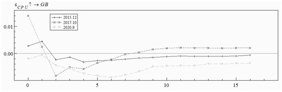
Figure 12.
Impact of CPU on GB at different points in time.
5.4. Robustness Check
In the VAR model, the choice of indicators will have an impact on the empirical results. To improve credibility, the volatility (QH) of the China Bond climate-related bond index was used as a proxy variable for the robustness test in this study. The constituent bonds of the China Bond Climate Related Bond Index are bonds that mainly satisfy one of the criteria of the Green Bond Support Project Catalogue and the Climate Bond Classification Scheme.
Comparing Figure 11 and Figure 13, the trends of the shocks of CPU on climate bond price volatility remain largely consistent with the previous section, especially in the short and medium term, where the results are very similar. Taking the short-term (0-month) constraint as an example, the price volatility affected by CPU of both climate bonds and green bonds reaches its extreme value around 2018, with an overall “up-down” trend in all three phases. Comparing Figure 12 and Figure 14, the impact of CPU on climate bond price volatility at three points in time is also largely consistent with the impact on green bond price volatility.
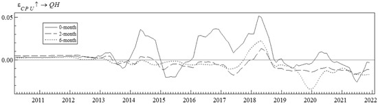
Figure 13.
Time-varying impulse response of CPU to QH.

Figure 14.
Impacts of CPU on QH at different points in time.
6. Conclusions
This study takes green bond price volatility as the research object and adopts the TVP-VAR model to explore the relationship between the impact of CPU on green bond volatility over time. The empirical results show that: (1) The impact of CPU on green bond price volatility is time-varying. In the short term, the impact is dramatic, and in the medium and long term it decreases green bond price volatility and the impact is reversed. From a behavioral finance perspective, this phenomenon may be caused by short-term overreaction or underreaction and is tempered in the medium to long term. From an investment specificity perspective, this phenomenon may be due to the overall direction of climate policy adjustment toward supporting the development of green bond markets and reducing price volatility. (2) By analyzing the impulse responses of CPU and shocks to green bond price volatility at different points in time, we found that CPU in the period of the Paris Agreement meeting in December 2015 and the release of the Annual Report in October 2017 had a positive impact on green bond price volatility from the beginning to a negative one after two periods. CPU on green bond price volatility during the period of the “double carbon” policy is generally negative and gradually stabilizes, and the impact is somewhat persistent.
This study mainly discusses that investors in the green bond market are rational people who will change their investment strategies as climate policies change. However, in reality there are still many “green” investors in the market, namely sustainable investors. When climate policy changes, the investment sentiment of rational investors may change, but for those green investors, they are more concerned about the “green” benefits of green bonds themselves and believe that green bonds have “green” core values, that is, green bonds can well resist the uncertainty caused by climate policy changes. They seem not to be so sensitive to climate policy changes, and the degree of uncertainty seems to be reduced. At this time, there may be some deviations in the applicability and universality of the conclusion that CPU affects green bond price fluctuations through investor sentiment. Moreover, to address climate change problems, Vuong [41] suggested embracing a new cultural core value centered around environmental protection. These are also possible limitations of this study. Therefore, our future studies can examine the specific research and analysis of investor behavior in different markets and corporate culture.
In fact, this paper mainly examines the relationship between climate policy uncertainty and green bond price volatility in a macro context, and fits more from the perspective of model regression to analyze the relationship between climate policy uncertainty and green bond volatility. Therefore, on the basis of the above findings, this study makes the following policy recommendations: (1) Conduct climate risk stress tests. By simulating various possible extreme weather scenarios and transition risks, climate change risk exposure can be analyzed prospectively, potential losses can be predicted, and countermeasures can be taken, thus reducing the impact of future climate policy adjustments and improving the resilience of the financial system; (2) Cultivate long-term “green” investors. For “green” speculators in the market, the relevant departments should guide them to become long-term “green” investors, and try to avoid the situation of short-term violent price fluctuations in the green bond market caused by investor panic due to the failure of climate policy; (3) strengthen the regulatory mechanism of the green bond market. Since climate policy uncertainties can significantly affect green bond price fluctuations in the short term, relevant regulatory authorities should strengthen the supervision of green bond market operations and pay timely attention to investor sentiment and the introduction of relevant policies, so as to alleviate green bond market turbulence.
Author Contributions
J.Y., methodology, software, resources, data curation, writing—original draft, visualization; M.Z., conceptualization, writing—supervision, project administration, funding acquisition; R.L., software, validation, formal analysis; G.W., investigation, writing—review and editing. All authors have read and agreed to the published version of the manuscript.
Funding
This paper was support by the National Natural Science Foundation of China (71961004); Postgraduate Research & Practice Innovation Program of Jiangsu Province (SJCX22_1517); and Science Foundation of Suzhou University of Science and Technology Grant (332111807, 332111801).
Data Availability Statement
Green bond price index can be obtained from the WIND database. CPU can be obtained from Economic Policy Uncertainty Index (http://www.policyuncertainty.com/climate_uncertainty.html, accessed on 16 November 2022).
Acknowledgments
The authors thank the editor and three anonymous reviewers of this study for their constructive suggestions and comments.
Conflicts of Interest
No potential conflict of interest was reported by the authors.
References
- Liu, M. The driving forces of green bond market volatility and the response of the market to the COVID-19 pandemic. Econ. Anal. Policy 2022, 75, 288–309. [Google Scholar] [CrossRef]
- Tian, H.; Long, S.; Li, Z. Asymmetric effects of CPU, infectious diseases-related uncertainty, crude oil volatility, and geopolitical risks on green bond prices. Financ. Res. Lett. 2022, 48, 103008. [Google Scholar] [CrossRef]
- Somanathan, E.; Somanathan, R.; Sudarshan, A.; Tewari, M. The impact of temperature on productivity and labor supply: Evidence from Indian manufacturing. J. Political Econ. 2021, 129, 1797–1827. [Google Scholar] [CrossRef]
- Bouri, E.; Iqbal, N.; Klein, T. CPU and the price dynamics of green and brown energy stocks. Financ. Res. Lett. 2022, 47, 102740. [Google Scholar] [CrossRef]
- Liang, C.; Umar, M.; Ma, F.; Huynh, T. CPU and world renewable energy index volatility forecasting. Technol. Forecast. Soc. Chang. 2022, 182, 121810. [Google Scholar] [CrossRef]
- Pham, L. Is it risky to go green? A volatility analysis of the green bond market. J. Sustain. Finance Invest. 2016, 6, 263–291. [Google Scholar] [CrossRef]
- Pham, L.; Huynh, T.L.D. How does investor attention influence the green bond market? Financ. Res. Lett. 2020, 35, 101533. [Google Scholar] [CrossRef]
- Larcker, D.F.; Watts, E.M. Where’s the greenium? J. Account. Econ. 2020, 69, 101312. [Google Scholar] [CrossRef]
- Tang, D.Y.; Zhang, Y. Do shareholders benefit from green bonds? J. Corp. Financ. 2020, 61, 101427. [Google Scholar] [CrossRef]
- Wang, J.; Chen, X.; Li, X.; Yu, J.; Zhong, R. The market reaction to green bond issuance: Evidence from China. Pac.-Basin Financ. J. 2020, 60, 101294. [Google Scholar] [CrossRef]
- Zerbib, O.D. The effect of pro-environmental preferences on bond prices: Evidence from green bonds. J. Bank. Financ. 2019, 98, 39–60. [Google Scholar] [CrossRef]
- Flammer, C. Corporate green bonds. J. Financ. Econ. 2021, 142, 499–516. [Google Scholar] [CrossRef]
- Jakubik, P.; Uguz, S. Impact of green bond policies on insurers: Evidence from the European equity market. J. Econ. Financ. 2021, 45, 381–393. [Google Scholar] [CrossRef]
- Jin, J.; Han, L.; Wu, L.; Zeng, H. The hedging effect of green bonds on carbon market risk. Int. Rev. Financ. Anal. 2020, 71, 101509. [Google Scholar] [CrossRef]
- Reboredo, J.C. Green bond and financial markets: Co-movement, diversification and price spillover effects. Energy Econ. 2018, 74, 38–50. [Google Scholar] [CrossRef]
- Reboredo, J.C.; Ugolini, A. Price connectedness between green bond and financial markets. Econ. Model. 2020, 88, 25–38. [Google Scholar] [CrossRef]
- Saeed, T.; Bouri, E.; Alsulami, H. Extreme return connectedness and its determinants between clean/green and dirty energy investments. Energy Econ. 2021, 96, 105017. [Google Scholar] [CrossRef]
- Wang, Q.; Zhou, Y.; Luo, L.; Ji, J. Research on the factors affecting the risk premium of China’s green bond issuance. Sustainability 2019, 11, 6394. [Google Scholar] [CrossRef]
- MacAskill, S.; Roca, E.; Liu, B.; Stewart, R.A.; Sahin, O. Is there a green premium in the green bond market? Systematic literature review revealing premium determinants. J. Clean. Prod. 2021, 280, 124491. [Google Scholar] [CrossRef]
- Xia, Y.; Ren, H.; Li, Y.; He, L.; Liu, N. Forecasting green bond volatility via novel heterogeneous ensemble approaches. Expert Syst. Appl. 2022, 204, 117580. [Google Scholar] [CrossRef]
- Kanamura, T. Are green bonds environmentally friendly and good performing assets? Energy Econ. 2020, 88, 104767. [Google Scholar] [CrossRef]
- Naeem, M.A.; Conlon, T.; Cotter, J. Green bonds and other assets: Evidence from extreme risk transmission. J. Environ. Manag. 2022, 305, 114358. [Google Scholar] [CrossRef]
- Tiwari, A.K.; Abakah, E.J.A.; Gabauer, D.; Dwumfour, R.A. Dynamic spillover effects among green bond, renewable energy stocks and carbon markets during COVID-19 pandemic: Implications for hedging and investments strategies. Glob. Financ. J. 2022, 51, 100692. [Google Scholar] [CrossRef]
- Elsayed, A.H.; Naifar, N.; Nasreen, S.; Tiwari, A.K. Dependence structure and dynamic connectedness between green bonds and financial markets: Fresh insights from time-frequency analysis before and during COVID-19 pandemic. Energy Econ. 2022, 107, 105842. [Google Scholar] [CrossRef]
- Choi, D.; Gao, Z.; Jiang, W. Attention to global warming. Rev. Financ. Stud. 2020, 33, 1112–1145. [Google Scholar] [CrossRef]
- Hong, H.; Li, F.W.; Xu, J. Climate risks and market efficiency. J. Econom. 2019, 208, 265–281. [Google Scholar] [CrossRef]
- Painter, M. An inconvenient cost: The effects of climate change on municipal bonds. J. Financ. Econ. 2020, 135, 468–482. [Google Scholar] [CrossRef]
- Seltzer, L.; Starks, L.T.; Zhu, Q. Climate Regulatory Risk and Corporate Bonds. In NBER Working Paper; NEBR: Cambridge, MA, USA, 2022. [Google Scholar]
- Huynh, T.D.; Xia, Y. Climate change news risk and corporate bond returns. J. Financ. Quant. Anal. 2021, 56, 1985–2009. [Google Scholar] [CrossRef]
- Barnett, M.; Brock, W.; Hansen, P.L. Pricing Uncertainty Induced by Climate Change. Rev. Financ. Stud. 2020, 33, 1024–1066. [Google Scholar] [CrossRef]
- Barro, R.J. Environmental protection, rare disasters and discount rates. Economica 2015, 82, 1–23. [Google Scholar] [CrossRef]
- Primiceri, G.E. Time varying structural vector autoregressions and monetary policy. Rev. Econ. Stud. 2005, 72, 821–852. [Google Scholar] [CrossRef]
- Nakajima, J. Time-Varying Parameter VAR Model with Stochastic Volatility: An Overview of Methodology and Empirical Applications. Monet. Econ. Stud. 2011, 29, 107–142. [Google Scholar]
- Bitto, A.; Frühwirth-Schnatter, S. Achieving shrinkage in a time-varying parameter model framework. J. Econom. 2019, 210, 75–97. [Google Scholar] [CrossRef]
- Jebabli, I.; Arouri, M.; Teulon, F. On the effects of world stock market and oil price shocks on food prices: An empirical investigation based on TVP-VAR models with stochastic volatility. Energy Econ. 2014, 45, 66–98. [Google Scholar] [CrossRef]
- Vuong, Q.H.; Nguyen, M.H.; La, V.P. The Mindsponge and BMF Analytics for Innovative Thinking in Social Sciences and Humanities; De Gruyter: Berlin, Germany, 2022. [Google Scholar]
- Gavriilidis, K. Measuring Climate Policy Uncertainty. Available online: https://www.policyuncertainty.com/climate_uncertainty.html (accessed on 16 November 2022).
- Ren, X.; Zhang, X.; Yan, C.; Gozgor, G. CPU and firm-level total factor productivity: Evidence from China. Energy Econ. 2022, 113, 106209. [Google Scholar] [CrossRef]
- Aye, G.C.; Balcilar, M.; Demirer, R.; Gupta, R. Firm-level political risk and asymmetric volatility. J. Econ. Asymmetries 2018, 18, e00110. [Google Scholar] [CrossRef]
- Gkillas, K.; Gupta, R.; Wohar, M.E. Volatility jumps, The role of geopolitical risks. Financ. Res. Lett. 2018, 27, 247–258. [Google Scholar] [CrossRef]
- Vuong, Q.H. The Semiconducting principle of monetary and environmental values exchange. Econ. Bus. Lett. 2021, 10, 284–290. [Google Scholar] [CrossRef]


Disclaimer/Publisher’s Note: The statements, opinions and data contained in all publications are solely those of the individual author(s) and contributor(s) and not of MDPI and/or the editor(s). MDPI and/or the editor(s) disclaim responsibility for any injury to people or property resulting from any ideas, methods, instructions or products referred to in the content. |
© 2023 by the authors. Licensee MDPI, Basel, Switzerland. This article is an open access article distributed under the terms and conditions of the Creative Commons Attribution (CC BY) license (https://creativecommons.org/licenses/by/4.0/).