Connected Intelligent Transportation System Model to Minimize Societal Cost of Travel in Urban Networks

Abstract

The increasing societal cost of vehicle travel in urban networks is causing higher social and environmental impacts on road users and urban residents. The societal cost of travel can be reduced through implementation of more efficient traffic management solutions, deeper integration of connected vehicles in the traffic stream, and increased deployment of vehicle-to-infrastructure (V2I) systems. This work proposes an innovative traffic management solution, based on Urban Connected Intelligent Transport Systems. The solution dynamically manages traffic by controlling for speed and acceleration in connected vehicles through V2I to minimize societal cost in urban networks. This is achieved by minimizing all four components of societal cost of travel, i.e., traffic accidents, fuel consumption, pollutant emissions and travel time. By minimizing societal cost, this research contributes to safer, greener and more sustainable transport in urban networks, while reducing the adverse environmental and economic impact. Experimental and field data as well as data from simulation were used to test the proposed solution at an urban coastal area in Patras, Greece.

1. Introduction

The rapid economic growth and the increased development of motorized transport has led to negative impacts on the environment and society [1]. Demand exceeds infrastructure capacity, generating congestion and traffic delays, high fuel consumption, a rise in greenhouse gas emissions and more accidents. The inefficient traffic management in urban road networks and the associated increased societal cost of travel result in social and environmental [2] impacts that burden drivers and passengers, as well as the residents of living areas.

Societal cost of travel can be reduced through implementation of more efficient traffic management solutions, deeper integration of connected vehicles in the traffic stream, and increased deployment of vehicle-to-infrastructure (V2I) systems [3]. The latest technological achievements and the evolution in communications networks are enhancing the implementation of Connected Intelligent Transport Systems (C-ITS) for traffic management, enabling continuous communication between vehicle users and the infrastructure.

The present study, going beyond the existing literature, analyses the societal cost of travel by automotive vehicles, excluding two-wheeled vehicles, in urban road networks, suggesting an innovative traffic management solution, the Urban Connected Intelligent Transport System (Urban C-ITS). In the literature, the estimation of the societal cost of travel is widely used in optimizing speed limits, but research has not adequately focused on the ways in which societal cost of travel can affect traffic management processes. Thus, this work contributes to the debate on the implementation of C-ITS models in smart cities and the reduction in the societal cost of travel in urban road networks.

The proposed Urban C-ITS dynamically manages traffic by imposing on connected vehicles, in real time through V2I systems, the necessary commands on the speed and the acceleration to be followed to minimize societal cost in an urban road network. In addition, the Urban C-ITS intervenes in traffic lights cycles by lengthening the green phase depending on the capacity and demand of the network, ensuring the minimum societal cost. Therefore, by minimizing the societal cost this research contributes to achieving greener, safer and more sustainable transport in urban road networks, and affecting both environmental and economic facets of society.

The factors constituting the societal cost of travel vary [4] depending on the scope and focus of a study. However, they always impact on critical social sectors such as health, safety, quality of life, the environment and the economy. The societal cost of travel has been studied mostly in Norway and Sweden, where it has been used in assessing the optimal speed limits [5]. The factors influencing the societal cost of travel were travel time, vehicle operating cost, traffic accidents, and noise and air pollution.

Further, the personal and external (societal) costs and benefits of travelling at high speed in motorways have been studied [6]. Although high speed causes increased external costs (pollution, bad health effects and increased risk of accident), drivers are sensitive only to personal benefit (saving time) and cost (fuel consumption, risk of injury) when selecting a travel speed.

For estimating the societal cost of urban travel, this research develops a model as function of the mean velocity and acceleration consisting of four factors: fuel consumption cost, pollutant emissions cost, traffic accidents cost and travel time cost. These are considered as the most important [7] determinants in the estimation of the societal cost of travel.

Indeed, the societal cost of travel in the urban environment is substantially affected by fuel consumption, as urban traffic is usually under urban traffic control that forces travelling drivers to stop and restart frequently. Beyond traffic control, interaction with pedestrians and micromobility users hamper drivers from maintaining a constant speed. Frequent deceleration and acceleration leads to increased fuel consumption, having long term impacts on the use of finite natural resources and on the economy. Critical in estimating societal cost of fuel consumption is the fuel type (e.g., petrol, diesel, electric power, LPG) consumed by the vehicles in the network, since each type of fuel requires a different estimation model of fuel consumption cost.

Vehicle emissions are largely responsible for air pollution, especially in urban areas where people and goods movements are higher; this represents a burden on the environment, citizens’ health and quality of life [8]. Therefore, the inclusion of the pollutant cost in the estimation of the societal cost of travel is considered of high importance.

The number of traffic accidents in Greece is high, while accidents have tragic consequences through loss of human life, injuries and property damage. From the statistics, the number of traffic accidents has been rising. Compared to other European countries, Greece ranks 20th of 27 in traffic safety [9]. Therefore, the factor of traffic accidents is critical in the estimation of the societal cost of travel and its minimisation leads to safer travel [10].

The cost of travel time is widely taken into account when estimating the societal cost of travel, since road users consider it as an important factor which is connected with the time they spend to commute or to engage in other daily social activities.

The overall performance and the outcomes of the proposed Urban C-ITS are assessed and discussed in the forthcoming sections, and two case studies are analysed. This article is structured as follows: in Section 2 the methodology and the modelling approach are presented; followed by a description of the study area and the data used in Section 3; the results along with the case studies are presented in Section 4; and the discussion and conclusions are provided in Section 5.

2. Methodology and Modelling Approach

This study develops the Urban C-ITS to minimize the societal cost of travel in urban networks, and thus the associated environmental and economic impacts. For the estimation of the societal cost of travel, a societal cost model is developed as a function of two random variables, the mean velocity and acceleration of automotive vehicles (personal and business cars, trucks and public transport buses) moving on a road network.

2.1. Modelling the Societal Cost of Travel

In this research, the societal cost of travel [EUR] consists of four factors: (a) cost [EUR] of fuel consumption (CFC), (b) cost [EUR] of pollutant emissions (CPE), (c) cost [EUR] of traffic accidents (CAc), and (d) cost [EUR] of travel time (CTT), as shown in Equation (1).

Societal Cost of Travel = k₁ ∗ CFC + k₂ ∗ CPE + k₃ ∗ CAc + k₄ ∗ CTT

(1)

where k_1–4 are weighting coefficients. If one or more factors are defined to have a higher effect than the others, these weighting coefficients should be quantified accordingly. In the literature, this quantification varies depending on the perspective of research on societal cost; for example, the perspective of the individual user moving on the road network or society’s perspective that is affected by the road traffic [5]. In this research, all factors contribute equally, and therefore, the weighting coefficients were all set equal to 1.0 [7].

2.1.1. Cost of Fuel Consumption

To estimate the cost of fuel consumption CFC, the types of fuel consumed by the vehicles in the network must first be defined. Each fuel type causes a different cost of fuel consumption. The total cost of fuel consumption composed of all fuel type costs is shown in Equation (2).

$$\mathrm{C}\mathrm{F}\mathrm{C}\left(\mathrm{V},\mathrm{a}\right)=\sum _{\mathrm{f}=1}^{\mathrm{n}}\left({\mathrm{F}\mathrm{C}}_{\mathrm{f}}\left(\mathrm{V},\mathrm{a}\right)\ast {\mathrm{W}}_{\mathrm{f}}\right)$$

(2)

where FC_f is the fuel consumption [mL] per type of fuel f as a function of mean velocity V [m/s] and acceleration a [m/s²]; and W_f is the unit cost of fuel f/[EUR/mL]. In this study, four types of fuel (associated with vehicle type) were defined: petrol cars, diesel cars, LPG cars and diesel trucks/buses; and the unit cost of each fuel f was 0.002094 EUR/mL for petrol, 0.002091 EUR/mL for diesel and 0.001004 EUR/mL for LPG [11]. Although both diesel cars and diesel trucks/buses use the same fuel type, their separate categorisation was needed since fuel consumption FC_f is estimated according to car type.

FC_f depends on the moving conditions of a vehicle, i.e., idling, travelling at constant speed, accelerating or decelerating [12,13,14], and is presented in Equation (3).

$${\mathrm{F}\mathrm{C}}_{\mathrm{f}}\left(\mathrm{V},\mathrm{a}\right)={[\mathrm{F}}_{\mathrm{i}}\ast {\Delta \mathrm{t}}_{\mathrm{i}}+{(\mathrm{c}}_1+{\mathrm{c}}_2\ast \mathrm{a}\ast \mathrm{V})\ast {\Delta \mathrm{t}}_{\mathrm{a}\mathrm{c}}+{(\mathrm{k}}_1\ast \left(1+\frac{{\mathrm{V}}^3}{2\ast {\mathrm{V}}_{\mathrm{m}}^3}\right)+{\mathrm{k}}_2\ast \mathrm{V})\ast {\Delta \mathrm{t}}_{\mathrm{c}\mathrm{r}}+{\mathrm{F}}_{\mathrm{d}}\ast {\Delta \mathrm{t}}_{\mathrm{d}}{]}_{\mathrm{f}}$$

(3)

where for each fuel/vehicle type f, F_i is vehicle idling consumption rate [mL/s]; Δt_i is vehicle idling time [s]; c₁ [mL/s] and c₂ [mL-s²/m²] are constants related to acceleration state; Δt_ac is vehicle acceleration time [s]; k₁ [mL/s] and k₂ [mL/m] are constants related to constant-speed state as described in Equations (4) and (5); V_m is the velocity at which the fuel consumption rate is at a minimum for vehicles cruising at constant speed [m/s]; Δt_cr is cruising at constant-speed vehicle time [s]; F_d is vehicle deceleration consumption rate [mL/s]; and Δt_d is vehicle deceleration time [s].

$${\mathrm{k}}_1=\frac{{(\mathrm{F}}_1-{\mathrm{F}}_2)\ast {\mathrm{V}}_1\ast {\mathrm{V}}_2\ast {\mathrm{V}}_{\mathrm{m}}^3}{180\ast (2\ast {\mathrm{V}}_2\ast {\mathrm{V}}_{\mathrm{m}}^3-{2\ast \mathrm{V}}_1\ast {\mathrm{V}}_{\mathrm{m}}^3+{\mathrm{V}}_2\ast {\mathrm{V}}_1^3-{\mathrm{V}}_1\ast {\mathrm{V}}_2^3)}$$

(4)

$${\mathrm{k}}_2=\frac{2{ \ast \mathrm{F}}_2\ast {\mathrm{V}}_2\ast {\mathrm{V}}_{\mathrm{m}}^3-{2\ast {\mathrm{F}}_1\ast \mathrm{V}}_1\ast {\mathrm{V}}_{\mathrm{m}}^3+{\mathrm{F}}_2\ast {\mathrm{V}}_2\ast {\mathrm{V}}_1^3-{\mathrm{F}}_1{\ast \mathrm{V}}_1\ast {\mathrm{V}}_2^3}{360\ast (2\ast {\mathrm{V}}_2\ast {\mathrm{V}}_{\mathrm{m}}^3-{2\ast \mathrm{V}}_1\ast {\mathrm{V}}_{\mathrm{m}}^3+{\mathrm{V}}_2\ast {\mathrm{V}}_1^3-{\mathrm{V}}_1\ast {\mathrm{V}}_2^3)}$$

(5)

For each fuel/vehicle type f, in Equations (4) and (5), F₁ is fuel consumption rate in litres per 100 km [L/100 km] for vehicles traveling at constant speed V_1, where V₁ = 90 km/h, and F₂ is fuel consumption rate in litres per 100 km [l/100 km] for vehicles traveling at constant speed V₂, where V₂ = 120 km/h, and V_m in km/h.

To estimate FC_f, through Equations (3)–(5), the values shown in

Table 1. Parameter values per fuel/vehicle type for fuel consumption estimation.

Fuel/Vehicle Type	F1 [L/100 km]	F2 [L/100 km]	Vm [km/h]	Fi [mL/s]	c1 [mL/s]	c1 [mL-s2/m2]	Fd [mL/s]
petrol cars	7.5	8.8	50	0.33	0.42	0.26	0.53
diesel cars	5.1	5.7	50	0.20	0.31	0.16	0.42
LPG cars	9.0	12.0	50	0.25	0.78	0.46	0.95
diesel trucks/buses	27.0	42.4	40	0.60	0.74	0.49	0.90

are suggested based on an extended literature review [15,16,17,18,19,20].

2.1.2. Cost of Pollutant Emissions

To estimate the cost of pollutant emissions CPE, the pollutants must first be defined, as well as the types of fuel consumed by the vehicles in the network. The pollutant emissions cost of each pollutant per type of fuel is estimated following Equation (6).

$$\mathrm{C}\mathrm{P}\mathrm{E}\left(\mathrm{V},\mathrm{a}\right)=\sum _{\mathrm{p}=1}^{\mathrm{m}}\sum _{\mathrm{f}=1}^{\mathrm{n}}\left({\mathrm{P}\mathrm{E}}_{\mathrm{p},\mathrm{f}}\left(\mathrm{V},\mathrm{a}\right)\ast {\mathrm{W}}_{\mathrm{p}}\right)$$

(6)

where PE_p,f is the pollutant emissions [g] of pollutant p and fuel/vehicle type f as a function of mean velocity V [m/s] and acceleration a [m/s²]; and W_p is the unit cost of pollutant p [EUR/g]. In this research, four pollutants were studied: (a) carbon dioxide—CO₂; (b) nitrogen oxides—NO_x; (c) volatile organic compounds—VOC; and (d) particulate matter—PM. As for the fuel/vehicle type, petrol cars, diesel cars, LPG cars and diesel trucks/buses were considered, similarly to Section 2.1.1. The unit cost of each pollutant p capturing the health impacts on people was 0.0028 EUR/g for CO₂, 0.0072 EUR/g for NO_x, 0.00012 EUR/g for VOC, and 0.1227 EUR/g for PM [21]. PE_p,f [22] is calculated according to Equation (7).

$${\mathrm{P}\mathrm{E}}_{\mathrm{p},\mathrm{f}}\left(\mathrm{V},\mathrm{a}\right)=\sum _{\mathrm{p}=1}^{\mathrm{m}}\sum _{\mathrm{f}=1}^{\mathrm{n}}\left({\mathrm{E}\mathrm{R}}_{\mathrm{p},\mathrm{f}}\left(\mathrm{V},\mathrm{a}\right)\ast \Delta \mathrm{t}\right)$$

(7)

where ER_p,f is the emission rate [g/s] of pollutant p and fuel/vehicle type f as a function of mean velocity V [m/s] and acceleration a [m/s²] as per Equation (8); and Δt is the time during which pollutant p was produced [s].

$${\mathrm{E}\mathrm{R}}_{\mathrm{p},\mathrm{f}}\left(\mathrm{V},\mathrm{a}\right)={\max \left[{\mathrm{E}}_0,{\mathrm{f}}_1+{\mathrm{f}}_2\ast \mathrm{V}+{\mathrm{f}}_3\ast {\mathrm{V}}^2+{\mathrm{f}}_4\ast \mathrm{a}+{\mathrm{f}}_5\ast {\mathrm{a}}^2+{\mathrm{f}}_6\ast \mathrm{V}\ast \mathrm{a}\right]}_{\mathrm{p},\mathrm{f}}$$

(8)

In Equation (8), E₀ is the minimum value of pollutant emission p and fuel/vehicle type f; and f_1–6 are constants related to pollutant emission p and fuel/vehicle type f. Their values, as used in this study, are summarized in

Table 2. Values of constants for CO₂ emission estimation.

Fuel/Vehicle Type	E0	f1	f2	f3	f4	f5	f6
petrol car	0	0.553	0.161	−0.00289	0.266	0.511	0.183
diesel car	0	0.324	0.086	0.00496	−0.059	0.448	0.230
LPG car	0	0.600	0.219	−0.00774	0.357	0.514	0.170
diesel truck/bus	0	1.520	1.880	−0.0695	4.710	5.880	2.090

,

Table 3. Values of constants for NO_x emission estimation.

Fuel/Vehicle Type	Acceleration [m/s2]	E0	f1	f2	f3	f4	f5	f6
petrol car	α ≥ −0.5	0	6.19 × 10−4	8.00 × 10−5	−4.03 × 10−6	−4.13 × 10−4	3.80 × 10−4	1.77 × 10−4
	α < −0.5	0	2.17 × 10−4	0	0	0	0	0
diesel car	α ≥ −0.5	0	2.41 × 10−3	−4.11 × 10−4	6.73 × 10−5	−3.07 × 10−3	2.14 × 10−3	1.50 × 10−3
	α < −0.5	0	1.68 × 10−3	−6.62 × 10−5	9.00 × 10−6	2.50 × 10−4	2.91 × 10−4	1.20 × 10−4
LPG car	α ≥ −0.5	0	8.92 × 10−4	1.61 × 10−5	−8.06 × 10−7	−8.23 × 10−5	7.60 × 10−5	3.54 × 10−5
	α < −0.5	0	3.43 × 10−4	0	0	0	0	0
diesel truck/bus		0	0.0356	9.71 × 10−3	−2.40 × 10−4	0.0326	0.0133	0.0115

,

Table 4. Values of constants for VOC emission estimation.

Fuel/Vehicle Type	Acceleration [m/s2]	E0	f1	f2	f3	f4	f5	f6
petrol car	α ≥ −0.5	0	4.47 × 10−3	7.32 × 10−7	−2.87 × 10−8	−3.41 × 10−6	4.94 × 10−6	1.66 × 10−6
	α < −0.5	0	2.63 × 10−3	0	0	0	0	0
diesel car	α ≥ −0.5	0	9.22 × 10−5	9.09 × 10−6	−2.29 × 10−7	−2.20 × 10−5	1.69 × 10−5	3.75 × 10−6
	α < −0.5	0	5.25 × 10−5	7.22 × 10−6	−1.87 × 10−7	0	−1.02 × 10−5	−4.22 × 10−6
LPG car	α ≥ −0.5	0	0.0144	1.74 × 10−7	−6.82 × 10−9	−8.11 × 10−7	1.18 × 10−6	3.96 × 10−7
	α < −0.5	0	8.42 × 10−3	0	0	0	0	0
diesel truck/bus		0	1.04 × 10−3	4.87 × 10−4	−1.49 × 10−5	1.27 × 10−3	2.10 × 10−4	1.00 × 10−4

and

Table 5. Values of constants for PM emission estimation.

Fuel/Vehicle Type	E0	f1	f2	f3	f4	f5	f6
petrol car	0	0	1.57 × 10−5	−9.21 × 10−7	0	3.75 × 10−5	1.89 × 10−5
diesel car	0	0	3.13 × 10−4	−1.84 × 10−5	0	7.50 × 10−4	3.78 × 10−4
LPG car	0	0	1.57 × 10−5	−9.21 × 10−7	0	3.75 × 10−5	1.89 × 10−5
diesel truck/bus	0	2.14 × 10−4	3.35 × 10−4	−2.22 × 10−5	0.00207	0.0018	2.27 × 10−4

.

2.1.3. Cost of Traffic Accidents

Prior to this analysis, the types of traffic accidents should be defined. The most common types of accident in the literature are (a) fatal accidents (fa), (b) serious injury accidents (sea), (c) slight injury accidents (sla) and (d) property-only damage accidents (pdo). Traffic accidents cost CAc is estimated as a function of mean velocity V [m/s] as follows [10,23,24].

$$\mathrm{C}\mathrm{A}\mathrm{c}(\mathrm{V})={\left(\frac{\mathrm{V}}{{\mathrm{V}}_{\mathrm{R}\mathrm{e}\mathrm{f}}}\right)}^{\mathrm{e}\mathrm{x}\mathrm{p}1}\ast {\mathrm{n}}_{\mathrm{f}\mathrm{a}}\ast {\mathrm{W}}_{\mathrm{f}\mathrm{a}}+{\left(\frac{\mathrm{V}}{{\mathrm{V}}_{\mathrm{R}\mathrm{e}\mathrm{f}}}\right)}^{\mathrm{e}\mathrm{x}\mathrm{p}2}\ast {\mathrm{n}}_{\mathrm{s}\mathrm{e}\mathrm{a}}\ast {\mathrm{W}}_{\mathrm{s}\mathrm{e}\mathrm{a}}+{\left(\frac{\mathrm{V}}{{\mathrm{V}}_{\mathrm{R}\mathrm{e}\mathrm{f}}}\right)}^{\mathrm{e}\mathrm{x}\mathrm{p}3}\ast {\mathrm{n}}_{\mathrm{s}\mathrm{l}\mathrm{a}}\ast {\mathrm{W}}_{\mathrm{s}\mathrm{l}\mathrm{a}}+{\left(\frac{\mathrm{V}}{{\mathrm{V}}_{\mathrm{R}\mathrm{e}\mathrm{f}}}\right)}^{\mathrm{e}\mathrm{x}\mathrm{p}4}\ast {\mathrm{n}}_{\mathrm{p}\mathrm{d}\mathrm{o}}\ast {\mathrm{W}}_{\mathrm{p}\mathrm{d}\mathrm{o}}$$

(9)

where V_Ref is the mean velocity [m/s] when the accident occurred or, if these data are not available, the road speed limit; n_fa, n_sea, n_sla and n_pdo are the number of traffic accidents of each type of accident; W_fa, W_sea, W_sla and W_pdo are the unit cost of each type of accident [EUR/accident]; and exp_1–4 are constants of each type of accident. In this study, the considered types of accident are all injury accidents (aia), including any injury regardless of severity (merging serious injury accidents and slight injury accidents) and property-only damage accidents (pdo). The values of the constants [25] and the unit costs related to accidents in Greece [26] are shown in

Table 6. Values of constants and unit costs for traffic accidents cost estimation.

Type of Accident	Exponent—Exp	Unit Cost—W [EUR/Accident]
fatal	2.6	43,596
serious injury	1.5	28,616
slightly injury	1.0	18,060
property-only damage	0.8	1937
all injury	1.2	23,338

.

2.1.4. Cost of Travel Time

The cost of travel time CTT depends on the user’s trip purpose according to main category, i.e., work trips or pleasure trips. The type of vehicle and its passengers’ trip purpose are highly related. In Equation (10), for each vehicle type j (e.g., private car, bus, truck), T(V) is the travel time per traversed distance [s/m] as a function of velocity V [m/s]; p_pur is the percentage of passengers that travel for purpose pur; W_pur is the unit cost of travel time for purpose pur [EUR/s-person]; d is the total traversed distance per vehicle type j [m]; and x is the average vehicle occupancy of vehicle type j [person].

$$\sum _{\mathrm{j}=1}^{\mathrm{m}}\sum _{\mathrm{p}\mathrm{u}\mathrm{r}=1}^{\mathrm{n}}(\mathrm{T}\left(\mathrm{V}\right)\ast {{\mathrm{p}}_{\mathrm{p}\mathrm{u}\mathrm{r}}\ast \mathrm{W}}_{\mathrm{p}\mathrm{u}\mathrm{r}}\ast \mathrm{d}\ast \mathrm{x})$$

(10)

In this study, vehicle type j consists of cars, buses and trucks. Concerning the passengers of car and bus, the trip purpose varies between work or pleasure during the day, as shown in

Table 7. Percentage of passengers that travel for work or pleasure per time slot in Greece (Data from [27]).

Time Slots	Travel for Work	Travel for Pleasure
7.00–11.00	80%	20%
11.00–17.00	20%	80%
17.00–20.00	50%	50%
20.00–24.00	5%	95%
24.00–7.00	30%	70%

. It was considered that all truck passengers travel only for work purposes.

The average vehicle occupancy x was 1.75 passengers for private cars and 1.24 passengers for trucks in Greece [27]. In the case of Patras, the average vehicle occupancy for bus was 10 passengers. Regarding the unit cost of travel time Wpur, it was defined based on the net average hourly wage of year 2021 in Greece. It was equal to 0.00204 EUR/s-person for work purposes, and 0.00051 EUR/s-person for pleasure.

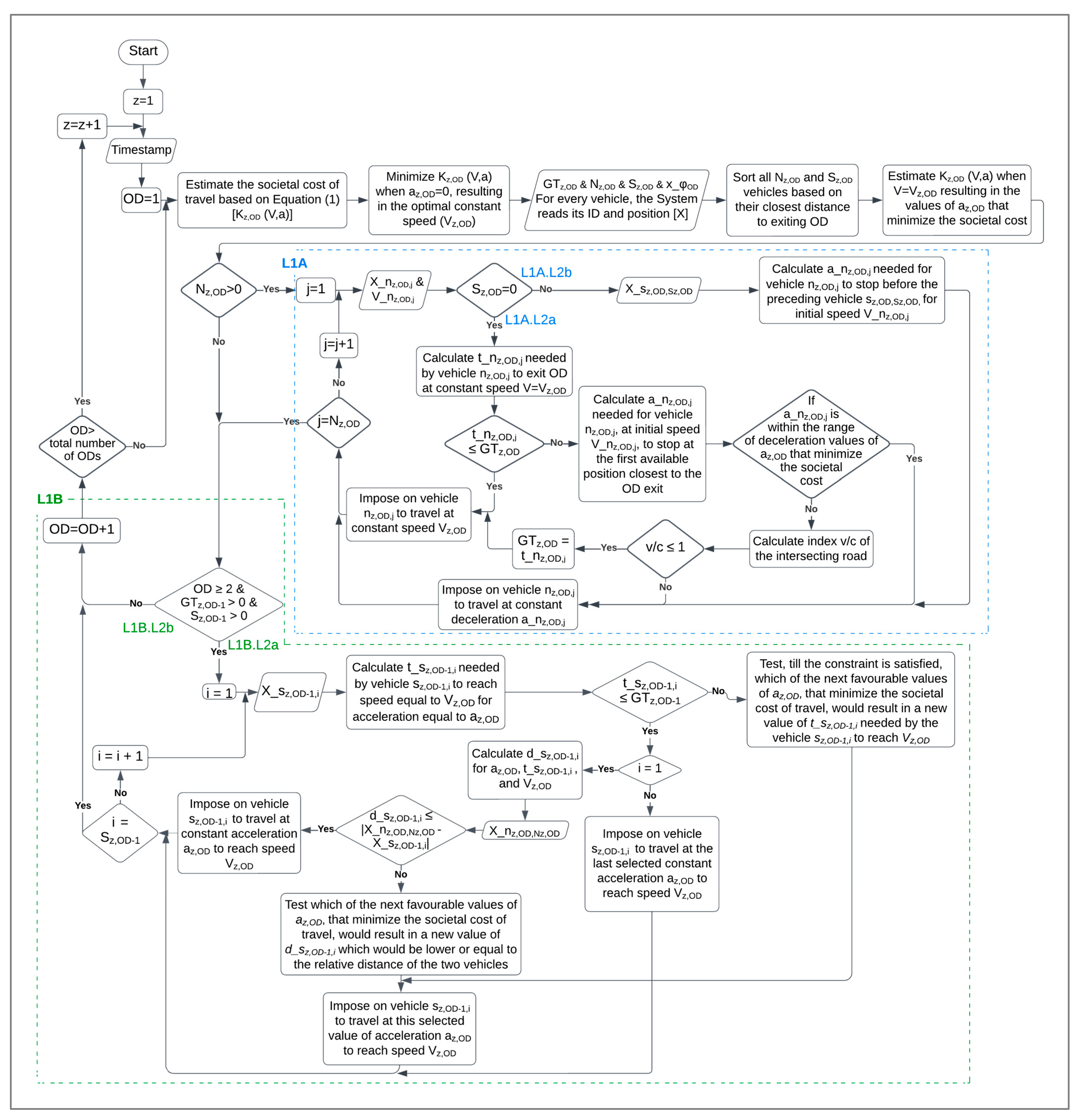
2.2. Innovative Urban Connected Intelligent Transport System

The Urban Connected Intelligent Transport System (Urban C-ITS) is applied to urban road networks consisting of a main road and secondary roads intersecting the main one at junctions with traffic lights. The iteration period interval (dt) must be defined. The System examines all sub-segments (OD) of the main road which are delimited by traffic lights. Through V2I technology, it imposes, in real time, on every connected vehicle that enters or moves on each OD the optimal velocity and/or acceleration to minimize the societal cost of travel till the next iteration, by utilizing mathematical optimization, respecting spatiotemporal traffic restrictions (i.e., movement of preceding vehicles and operation of traffic lights) but not allowing lane change.

When the minimization of the societal cost is not possible owing to traffic restrictions, the System intervenes in the OD traffic light’s cycle after assessing the index v/c for each road intersecting the main one. This index is the ratio of the traffic volume (v) to the traffic capacity (c). If the ratio v/c ≤ 1.0, then the System can extend the corresponding green phase time on the main road. The Urban C-ITS is presented in the flow chart of Figure 1.

The System reads the time and date (Timestamp) at every iteration (z). The model for the estimation of the societal cost of travel is configured based on time slots indicated in Table 7. Starting with the first OD, the System applies Equation (1) and estimates the societal cost of travel of the OD (K_z,OD (V,a)) as a function of mean velocity V and acceleration a. In each iteration (z), the formulated Equation (1) is the objective function to be minimized in next steps of the proposed Urban C-ITS, based on specific constraints defined in each step.

Next it minimizes the societal cost K_z,OD (V,a) (objective function) with the constraint that a_z,OD equals to zero, resulting in the optimal constant speed (V_z,OD).

The System reads the remaining green time (GT_z,OD) of the traffic light at the end of OD. It reads the total number of vehicles moving on the OD (N_z,OD) and the total number of vehicles idling at the end of the OD owing to red traffic light (S_z,OD). For every vehicle, the System reads its ID and position. This separation is necessary as there follow steps that differ according to the whether the vehicles are already in motion or are idling and have to accelerate to move and enter the next road sub-segment at the next iteration. Then, N_z,OD vehicles and S_z,OD vehicles are sorted based on their closest distance to exiting OD.

A single system for measuring the positions of vehicles in all ODs must be defined. The position of each vehicle defined from the beginning of the front bumper to the end of the rear bumper needs to be recorded. When the System calculates the relative distance (gap) between two vehicles, this is calculated as the difference of the position of the rear bumper of the preceding vehicle from the front bumper of the following vehicle. The position of the traffic light x_φ_OD is also read.

Next, the System estimates the societal cost K_z,OD (V,a) with the constraint that V equals to V_z,OD, resulting in the values of a_z,OD that minimize the societal cost. The conclusion in the literature [28] is that the lowest societal cost of travel is achieved when vehicles move either with constant speed or smoothly accelerating and decelerating. In this regard, the calculations below related to individual vehicle’s movement (e.g., distance, time) follow the fundamental equations of motion for the aforementioned cases.

• The first level of Case Classification (L1) refers to the existence of vehicles moving on the OD, N_z,OD.

  -

  L1A: If vehicles N_z,OD are moving on the OD

An iterative loop is activated. For every vehicle n_z,OD,j of this category (previously sorted), vehicle position X_n_z,OD,j and speed V_n_z,OD,j are read. The System checks if there are vehicles S_z,OD idling at the end of the OD owing to red traffic light.

• The second level of Case Classification (L2) of L1A refers to the existence of vehicles idling at the end of the OD owing to red traffic light, S_z,OD.

  —

  L1A.L2a: If there are no vehicles S_z,OD idling at the end of the OD

The time t_n_z,OD,j needed by vehicle n_z,OD,j to exit OD is calculated for traveling at constant speed equal to V_z,OD and given its current position X_n_z,OD,j. The System checks if vehicle n_z,OD,j traveling at constant speed V_z,OD will be able to exit OD with green light; i.e., it checks if time t_n_z,OD,j ≤ GT_z,OD.

If this check is valid, the System imposes on vehicle n_z,OD,j to travel at constant speed V_z,OD till the next iteration. At this point, the first loop iteration is completed, and the System continues the iterative loop for all next vehicles n_z,OD,j. If the aforementioned check is not valid, the System calculates the constant deceleration a_n_z,OD,j needed for vehicle n_z,OD,j, at initial speed V_n_z,OD,j, to stop at the first available position closest to the OD exit. If a_n_z,OD,j is within the range of deceleration values of a_z,OD that minimize the societal cost (previously estimated), the System imposes on vehicle n_z,OD,j to travel at constant deceleration a_n_z,OD,j. At this point, the first loop iteration is completed, and the System continues the iterative loop for all next vehicles n_z,OD,j.

If a_n_z,OD,j is out of the range of deceleration values of a_z,OD that minimize the societal cost (previously estimated), the System calculates the index v/c of the intersecting road. If v/c ≤ 1.0, the traffic state of the intersecting road permits the System to extend the corresponding green time on the main road. The time extension is equal to t_n_z,OD,j. The System imposes on vehicle n_z,OD,j to travel at constant speed V_z,OD till the next iteration. As a result, the unfavourable deceleration of vehicle n_z,OD,j causing high societal cost of travel is avoided. At this point, the first loop iteration is completed, and the System continues the iterative loop for all next vehicles n_z,OD,j. On the contrary, if v/c > 1.0, the heavy traffic conditions of the intersecting road do not permit the System to extend the corresponding green time on the main road. Thus, the vehicle n_z,OD,j will travel at constant deceleration a_n_z,OD,j. At this point, the first loop iteration is completed, and the System continues the iterative loop for all next vehicles n_z,OD,j.

•  

  —

  L1A.L2b: If there are vehicles S_z,OD idling at the end of the OD

The System reads last idling vehicle’s (${\mathrm{s}}_{{\mathrm{z},\mathrm{O}\mathrm{D},\mathrm{S}}_{\mathrm{z},\mathrm{O}\mathrm{D}}}$) position ${\mathrm{X}\_\mathrm{s}}_{{\mathrm{z},\mathrm{O}\mathrm{D},\mathrm{S}}_{\mathrm{z},\mathrm{O}\mathrm{D}}}$. Based on this position and n_z,OD,j vehicle’s position X_n_z,OD,j, the System calculates distance D_n_z,OD,j, which is available to vehicle n_z,OD,j to stop. Taking into account this distance and for initial speed V_n_z,OD,j, the System calculates the constant deceleration a_n_z,OD,j needed for vehicle n_z,OD,j to stop before the preceding vehicle ${\mathrm{s}}_{{\mathrm{z},\mathrm{O}\mathrm{D},\mathrm{S}}_{\mathrm{z},\mathrm{O}\mathrm{D}}}$. The System imposes on vehicle n_z,OD,j to travel at constant deceleration a_n_z,OD,j. At this point, the first loop iteration is completed, and the System continues the iterative loop for all next vehicles n_z,OD,j.

•  

  -

  L1B: If there are no vehicles N_z,OD moving on the OD or if all n_z,OD,j vehicles have been processed in the previous iterative loop

• The second level of Case Classification (L2) of L1B refers to the existence of remaining green time (GT_z,OD-1) of the traffic light at the end of OD-1.

  —

  L1B.L2a: If there is remaining green time GT_z,OD-1 of the traffic light at the end of OD-1

Next, the System analyses the vehicles s_z,OD-1,i which are idling at the traffic light at the end of main road’s previous sub-segment (OD-1) because of red light. These vehicles will accelerate to enter the OD sub-segment in the next time intervals. This analysis continues for all sub-segments under study; the constraint OD ≥ 2 must be applied since the analysis is not applicable when only one sub-segment is studied. Otherwise or if there no vehicles s_z,OD-1,i, the System follows the steps described in L1B.L2b.

This System’s loop starts when OD = 2 and there is remaining green time (GT_z,OD-1) of the traffic light at the end of OD-1, iterating for every vehicle s_z,OD-1,i (previously sorted) of category S_z,OD-1. In this iterative loop, data from both road sub-segments OD and OD-1 are needed. The vehicles idling at the red traffic light at the end of OD-1 should be analysed based on the equation of the societal cost of travel as formulated for the next sub-segment OD. Also, the acceleration of these vehicles is constrained by the traffic conditions of the next sub-segment OD.

For every vehicle s_z,OD-1,i, vehicle position X_s_z,OD-1,i is read. For acceleration a_z,OD that minimizes the societal cost of travel (previously estimated), the time t_s_z,OD-1,i needed by vehicle s_z,OD-1,i to reach speed equal to V_z,OD is calculated. At this point, the System checks if t_s_z,OD-1,i ≤ GT_z,OD-1.

If indeed t_s_z,OD-1,i ≤ GT_z,OD-1, and if I = 1, meaning that the first idling vehicle is being studied, then the System calculates the distance d_s_z,OD-1,i that this vehicle will traverse given that acceleration equals a_z,OD, time equals t_s_z,OD-1,i and speed equals V_z,OD. The System recalls the position ${\mathrm{X}\_\mathrm{n}}_{{\mathrm{z},\mathrm{O}\mathrm{D},\mathrm{N}}_{\mathrm{z},\mathrm{O}\mathrm{D}}}$ of the preceding vehicle, which is the position of the last moving vehicle on the next OD. If d_s_z,OD-1,i is less or equal to the relative distance (gap) of the two vehicles, then the System imposes on vehicle s_z,OD-1,i to travel at constant acceleration a_z,OD to reach the favourable speed V_z,OD. At this point, the first loop iteration is completed, and the System continues the iterative loop for all next vehicles s_z,OD-1,i. If d_s_z,OD-1,i is higher than the gap of the two vehicles, the System tests which of the next favourable values of a_z,OD, that minimize the societal cost of travel, would result in a new value of d_s_z,OD-1,i which would be lower or equal to the relative distance of the two vehicles. This selected value of a_z,OD is imposed on vehicle s_z,OD-1,i to reach V_z,OD. At this point, the first loop iteration is completed, and the System continues the iterative loop for all next vehicles s_z,OD-1,i. If indeed t_s_z,OD-1,i ≤ GT_z,OD-1, and i > 1, meaning that an idling vehicle, apart from the first one, is studied, the System imposes on vehicle s_z,OD-1,i to travel at the last selected constant acceleration a_z,OD to reach V_z,OD. At this point, the first loop iteration is completed, and the System continues the iterative loop for all next vehicles s_z,OD-1,i.

If constraint t_s_z,OD-1,i ≤ GT_z,OD-1 is not satisfied, the System tests, till the constraint is satisfied, which of the next favourable values of a_z,OD, that minimize the societal cost of travel, would result in a new value of t_s_z,OD-1,i needed by the vehicle s_z,OD-1,i to reach V_z,OD. For all studied vehicles except the first one, an additional limitation applies; the tests are performed up to the acceleration value obtained by the previous studied vehicle. The final selected favourable value of a_z,OD is imposed on vehicle s_z,OD-1,i to reach V_z,OD. At this point, the first loop iteration is completed, and the System continues the iterative loop for all next vehicles s_z,OD-1,i.

•  

  —

  L1B.L2b: If there is no remaining green time GT_z,OD-1 of the traffic light at the end of OD-1

The System continues to the next OD. When all ODs are analysed, the System proceeds to the next iteration z+1.

3. Study Area and Data

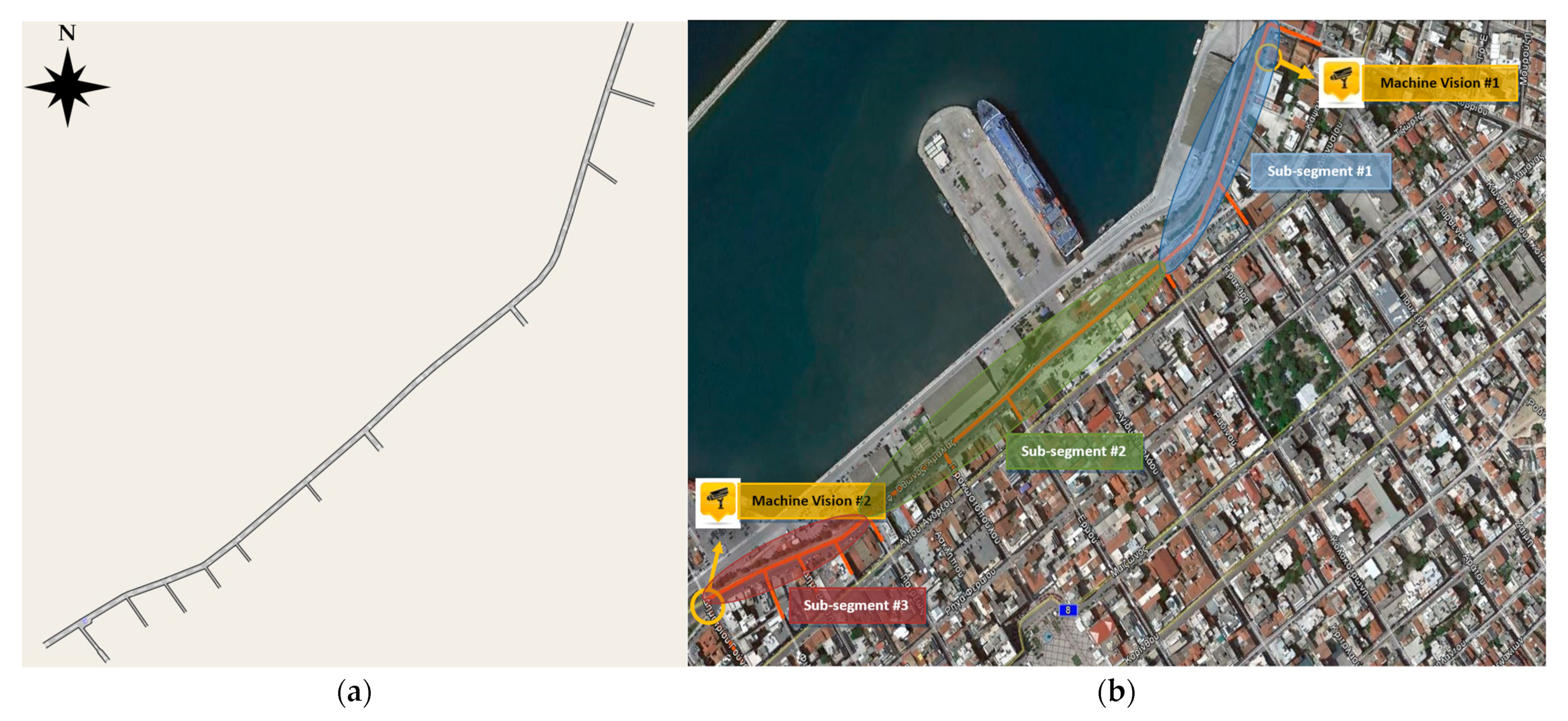
3.1. Study Area

In this research, the study area is a section of the main coastal urban road of Patras city, Greece: Othonos-Amalias avenue, bounded by the 28 October or Karolou intersecting street to Dimitriou Gounari intersecting avenue. Both the entrance and the exit of the study area are supervised by Machine Vision (MV) systems, each of which records traffic data. The model of the selected study area is shown in Figure 2a. The area under study is divided into three sub-segments delimited by traffic lights. The sub-segments and positions of the Machine Vision systems are shown in Figure 2b.

Sub-segment 1 is bounded by the 28 October or Karolou intersecting street to Kolokotroni intersecting street; Sub-segment 2 is bounded by Kolokotroni intersecting street to Patreos intersecting street; and Sub-segment 3 is bounded by Patreos intersecting street to Dimitriou Gounari intersecting avenue.

The city of Patras has an extensive beachfront, along which a coastal road network is being developed that serves a large volume of vehicles moving from one end of the city to the other. Othonos-Amalias avenue is used by travellers who move from areas north of the city such as Rio, to areas further south such as the southern port of Patras, Vrachneika and the Industrial Zone of Patras. It is also used by drivers heading out of Patras to nearby towns such as Amaliada and Pyrgos. In addition, users who want to avoid the urban centre of Patras choose Othonos-Amalias and turn onto the intersecting street which is their final destination. Of particular importance is the use of Othonos-Amalias by private and professional drivers heading to the southern port of Patras, which also explains the presence of heavy vehicles. From the above, the selected study area is a key avenue of the city, congested during peak hours.

The study area consists of two traffic lanes formed along its entire length. The width of each lane is at 3.5 m. The overall width of the avenue would allow vehicles to use a third lane, but the parked vehicles on the left side of the road do not allow this. The formation of a third traffic lane is observed at the point of the left turn onto Dimitriou Gounari avenue, i.e., shortly before the end of the study area. After that point, traffic continues in three lanes. Concerning public transport, several public bus routes traverse the study area, where the main train station is also located.

3.2. Data

In this study, multisource traffic-related data were used to implement the suggested methodological framework. The management of the data was as follows:

• Field data manually recorded: For developing a representative traffic simulation model, traffic flow and turning percentages data from the study area had to be collected. In particular, we measured the traffic flow entering the under study section of Othonos-Amalias avenue, the traffic flow entering Othonos-Amalias avenue from the intersecting roads and the turning flow exiting Othonos-Amalias avenue towards the intersecting roads. These data were recorded separately for the category of passenger vehicles and heavy vehicles, trucks and buses. The data were processed to obtain the exiting turning percentages. These data are shown in Tables S1 and S2 of Supplementary Materials.
• Traffic data from Machine Vision systems: Traffic volume, traffic flow and turning percentages were also collected by the two Machine Vision systems which monitor the entry and exit of the study area. The Machine Vision systems are parameterized to record traffic data per pre-defined vehicle classes by vehicle length. To adapt the recorded data into the vehicle categories of this study (i.e., passenger vehicles and heavy vehicles, trucks and buses) and insert them in the traffic simulation model, the data were processed as shown in Tables S3–S7 of Supplementary Materials.
• Data related to traffic lights at the intersections: It was necessary to record the cycle of each traffic light at the signalized intersections, including the duration of the individual traffic light phases. This information is needed for the development of the traffic simulation model. Location and operation data of each traffic light are shown in Table S8 of Supplementary Materials.
• Data related to public transport: For the traffic simulation of the study area, it was needed to record information on the routes of the city buses, and data on the average duration of the bus stops. The frequency of the routes (Table S9 of Supplementary Materials) was obtained from the official website of the urban transport authority of the city of Patras. The average stop duration was defined as 18 s based on field measurements of 45 buses that stopped at the bus stop located in the road segment under study.
• Traffic accidents: On the number of traffic accidents per category studied (all injury accidents (aia) including any injury regardless of severity and property-only damage accidents (pdo)), documentation from Patras Traffic Police was used to collect accident records as shown in Table S10 of Supplementary Materials.
• Open Street Maps were used to insert the study area in the traffic simulation software.

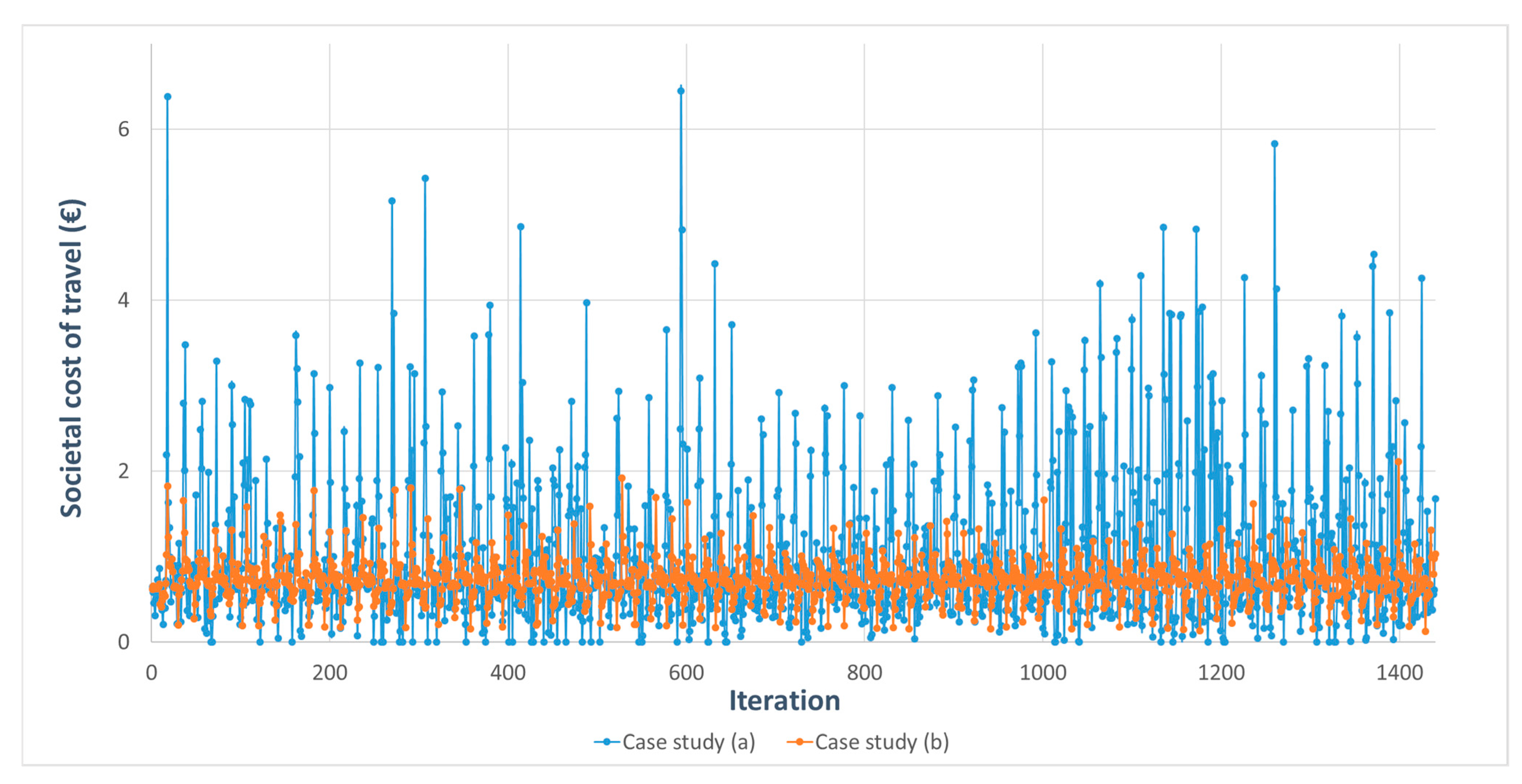
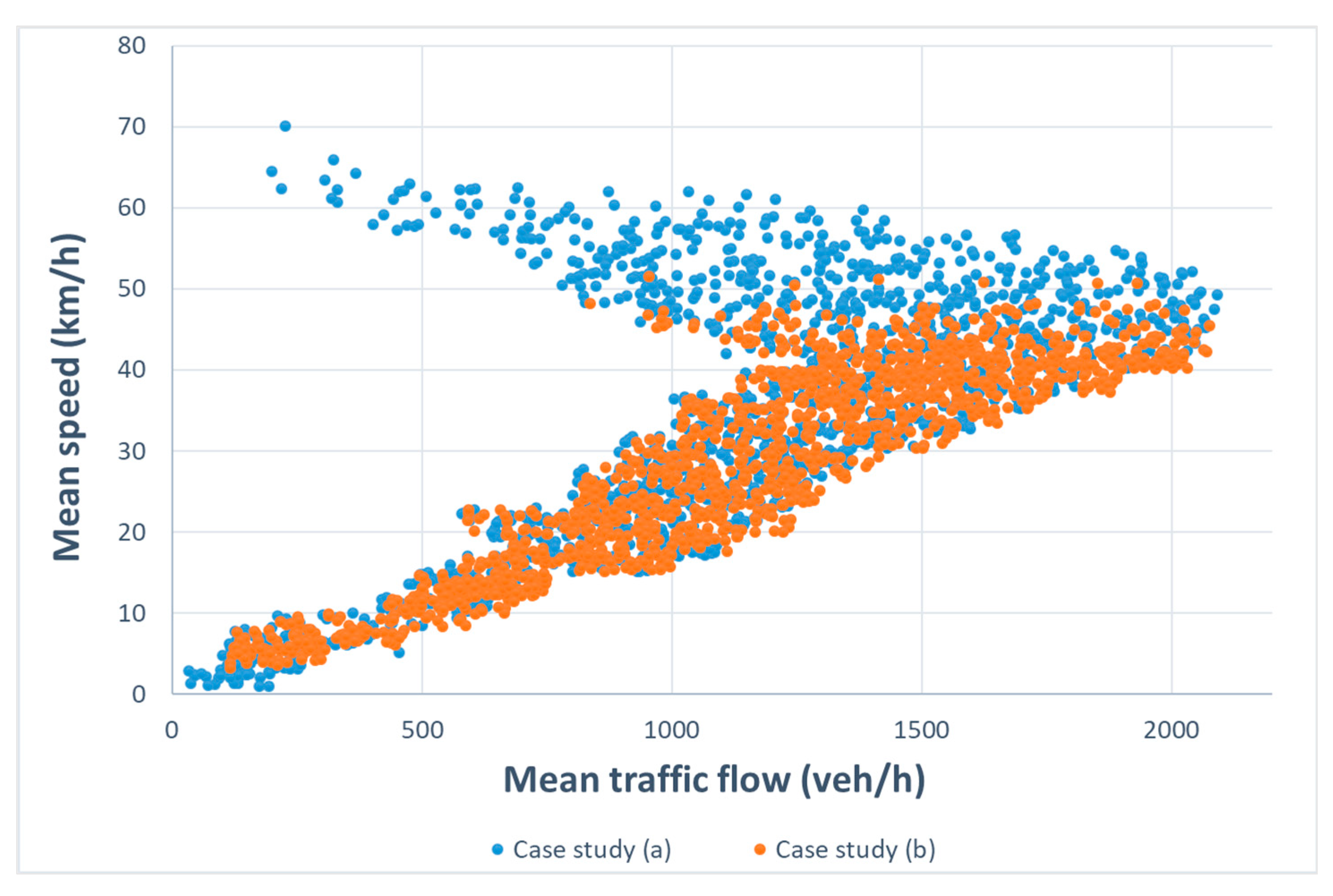
4. Results

Two case studies are analysed for the study area in Patras, Greece: Case study (a) without the application of the suggested Urban C-ITS, corresponding to current traffic conditions, and Case study (b) with the application of the suggested Urban C-ITS.

The results reported in this section demonstrate the influence of the suggested Urban C-ITS on traffic management, and on environmental and societal aspects, compared to current traffic conditions of the study area. A comparative evaluation enables us to quantify the impact deriving from the application of the proposed System, and draw useful conclusions. The evaluation indicators are the societal cost of travel, mean traffic flow, mean travel time, mean fuel consumption, total CO₂ emissions, total NO_x emissions, total VOC emissions and total PM emissions.

The study period is the same for both aforementioned cases: a weekday morning, from 9.00 a.m. to 11.00 a.m. The two case studies were simulated with traffic simulation software Aimsun Next 8.4.4.

Figure 3 illustrates the societal cost of travel (EUR) at each iteration (5 s) of the Urban C-ITS applied during the two-hour period of Case study (b); for the same time intervals, it depicts the societal cost of travel for Case study (a).

The values of the societal cost are reduced, for the majority of iterations in Case study (b) compared to Case study (a). In particular, there is significant reduction in the higher values of the societal cost that appeared in Case study (a), fulfilling the ultimate goal of the proposed Urban C-ITS. In Case study (b), where the System is applied, the majority of the societal cost values are between EUR 0.55 and EUR 0.85. This is justified by the System operation principles which form smooth traffic conditions reducing unnecessary sharp speed fluctuations and extreme values, resulting in societal cost estimations that do not vary substantially across iterations. At the iterations corresponding to yellow and red traffic light phases as well as the starting time of green phases (as shown in Tables S11–S16 of Supplementary Materials), when vehicles have to stop or restart, the societal cost values are greater and out of this range, but still lower compared to Case study (a). From the data, in Case study (a), the best adapted probability distribution is the generalized extreme value, while in Case study (b), the best is the Laplace distribution as demonstrated in Figure 4.

From Case study (a) in Figure 5, the same value of the mean traffic flow can be observed for a number of mean speed values. In particular, low mean traffic flow values are presented at very low and at very high mean speed values. This is justified by the fact that at very low speed values, the traffic flow served is low, as, for example, in congested traffic. Also, at low traffic flow values, vehicles can travel at a very high speed.

Further, the higher the traffic flow value, the more limited the range of speed values. For the highest observed traffic flow values, the speed values vary between 32 km/h and 58 km/h. The points of Case study (b), see Figure 5, follow a pattern similar to those of Case study (a); however, the majority of mean speed values do not exceed 50 km/h, and very few are slightly above this value. This is due to the proposed System operation which does not allow very high speed values as these values would increase the societal cost of travel. Additionally, all points of Case study (b) are slightly shifted to the right, compared to the points of Case study (a); i.e., when the suggested System is applied, at the same mean speed value, the mean traffic flow value is higher compared to the case where the System is not applied. Thus, the application of the System improves the traffic throughput of the road segment, i.e., more vehicles are served at the same mean speed.

Table 8. Evaluation indicators in each case study for the study period of two hours.

Evaluation Indicators	Case Study (a)	Case Study (b)	Percentage Change
Total societal cost of travel	EUR 1472.54	EUR 1053.39	(−) 28.46%
Total vehicles CO2 emissions	836,589 g	603,289 g	(−) 27.89%
Total vehicles NOx emissions	2638.6 g	2117.8 g	(−) 19.74%
Total vehicles VOC emissions	923.2 g	636.9 g	(−) 31.01%
Total vehicles PM emissions	215.8 g	147.3 g	(−) 31.74%
Average vehicle fuel consumption	0.149 L/veh	0.117 L/veh	(−) 21.48%
Average vehicle travel time	291 s	267 s	(−) 8.25%
Mean traffic flow	1124 veh/h	1137 veh/h	(+) 1.16%

summarizes the comparative evaluation results, presenting the values of the eight predefined evaluation indicators for both case studies. The evaluation indicator of the total societal cost of travel is equal to EUR 1472.54 in Case study (a), while in Case study (b), it equals EUR 1053.39. Thus, the application of the System leads to an estimated reduction of 28.46% in the societal cost of travel, i.e., in the desired direction in this research.

As for the direct impact on the environment and air quality, a considerable reduction in all four pollutants emissions is achieved in Case study (b) compared to Case study (a). Total vehicles CO₂ emissions are reduced by 27.89%, NO_x emissions by 19.74%, VOC emissions by 31.01% and PM emissions by 31.74%.

As for the indirect environmental impact in terms of the depletion of natural resources, the average vehicle fuel consumption is 0.149 L/veh in Case study (a) and 0.117 L/veh in Case study (b), resulting in a 21.48% reduction in vehicle fuel consumption when the System is applied. The average vehicle travel time is reduced by 8.25% as vehicles are crossing the under-study road segment faster by 24 s in Case study (b). The mean road traffic flow of the study area is 1124 veh/h in Case study (a), whereas in Case study (b), it is 1137 veh/h, i.e., increasing throughput by 1.16%, enabling more vehicles to be served.

5. Discussion

Environmentally burdened cities need innovative solutions to face their urgent sustainability challenges, and the share of the transport sector in this burden is high. Transportation causes substantial negative impacts on the environment and human health, being responsible for about a quarter of the EU’s total greenhouse gas (GHG) emissions, and causing air pollution and health risks [29]. In this framework, and considering the increasing traffic demand in urban road networks, the societal cost of travel should be systematically studied [28,30,31,32].

In particular, the societal cost of travel should be one of main elements used by transportation decision makers and engineers in designing transportation infrastructure and urban traffic management solutions. Traffic management plans and systems are often designed considering the design speed, the average travel time or the average delay per vehicle [33], leaving aside the societal costs related to environmental and air quality degradation, resources depletion and road users’ safety. Contrary to traditional approaches, the present study proposes an innovative urban traffic solution, the Urban Connected Intelligent Transport System (Urban C-ITS). The System dynamically manages traffic by imposing certain moving conditions on connected vehicles and by intervening in traffic signal control strategies based on the minimization of the societal cost of travel in the urban road network [1]. The suggested Urban C-ITS can contribute to the enhancement of urban transportation sustainability and the achievement of greener and safer urban travel.

For the estimation of the societal cost of travel, this research develops a societal cost model as a function of mean velocity and acceleration. The societal cost of travel consists of four factors: traffic accidents, fuel consumption, pollutant emissions and travel time. Each cost was estimated as a function of speed and/or acceleration of the vehicles moving in the urban network. The data of individual vehicles are easy to collect if all vehicles of the network are connected vehicles. As this was not the case in our application, the study area was simulated in Aimsun Next 8.4.4 traffic software using real traffic data collected from the study area primarily through Machine Vision systems.

The suggested Urban C-ITS, which incorporates the model of societal cost of travel, was applied to the study area in the urban road network of Patras, Greece. Two case studies were analysed: Case study (a): no-action case, corresponding to current traffic conditions; Case study (b): with application of the suggested Urban C-ITS. The study period is the same for both cases: a weekday morning, from 9.00 am to 11.00 am. The proposed methodology and modelling approach of this study is considered easily adjustable to the requirements of urban road networks with similar characteristics as the selected study area.

From the results, mean speed values varied in a smaller range after the application of the System, compared to the current no-action case, i.e., road operation without the System; implying that vehicle movements were smoother in Case study (b) compared to Case study (a). More specifically, less extreme mean speed values were observed when the System was responsible for traffic management.

In the no-action case, a large number of high mean speed values exceeding 50 km/h and several values exceeding 60 km/h was noted. In contrast, with the System’s application, the highest mean speed values reached up to 50 km/h and very few marginally exceeded this value. In summary, the proposed System leads to vehicle speeds between 30 km/h and 50 km/h. These values coincide with the current speed limits for the main types of road within an urban environment, and are consistent with the recent proposals of the National Road Safety Strategic Plan 2021–2030 [34] concerning speed limit reduction for urban roads.

In certain cases, the application of the proposed System led to the extension of the green phase of the main road of the study area in order to reduce the estimated societal cost. Nevertheless, very high values of societal cost of travel were rarely observed, and therefore, the System needed to intervene rarely.

The societal cost of travel was reduced in the vast majority of cases relative to the no-action case, mostly ranging between EUR 0.55 and EUR 0.85. This finding is justified by the System’s operation, which forms smooth traffic conditions without unnecessary sharp fluctuations and extreme speed values. This was not the case for orange and red phases as well as starting time of green phase. To be sure, when traffic control forces vehicles to stop, idle or restart, societal cost values increase; but in Case study (b), they are still lower compared to the no-action case study.

Overall, application of the proposed Urban C-ITS for the entire study period reduced total societal cost by almost 30%, indicating the viability of our hypothesis on its potential for achieving greener and safer urban travel. The results indicated considerable improvement of environmental performance, by a reduction between 20%–32% in all indicators, namely “Total vehicles CO₂ emissions”, “Total vehicles NO_x emissions”, “Total vehicles VOC emissions”, “Total vehicles PM emissions” and “Average vehicle fuel consumption”. Further, the System’s application led to a reduction in “Average vehicle travel time” of 8.25%. As travel time is directly perceived by the users, this reduction may contribute to future acceptance of the System’s application. Last, for the same mean speed value, a higher throughput is served in the case study with the System application compared to the no-action case study.

Certain prospects of this study are worthy of further discussion. First, the systematic entry of modern hybrid and electric vehicles will affect two of the factors in estimating the societal cost of travel. More specifically, these vehicle types are often considered to have reduced fuel (for hybrids) or energy (for purely electric) demand compared to conventional vehicles. As their fuel consumption and emissions behaviour cannot be described by the conventional models [35], it would be of interest to study their effect on these factors, and consequently on the overall societal cost in a mixed traffic or all-electric environment.

Another suggestion for further research would be the calculation of the exponents of Elvik’s model [10,24] for each study area from the very beginning. For this purpose, a large number and very detailed data on the conditions of the traffic accidents that take place in the study area would be needed. A comparative analysis between the existing exponent values and the estimated ones would result in estimating the impact of the exponents on the estimation of the societal cost of travel. In our study, this was not possible since no such detailed traffic accident data were recorded by Patras Traffic Police.

A further suggestion for research is related to the estimation of pollutant emissions. Some models estimate pollutant emissions by the slope of the road segment. In the present work, the selected study area does not exhibit a slope that could affect the results of the cost of pollutant emissions and thus the societal cost. However, if there is a considerable slope in the study area, researchers should use an appropriate model [36] in order to take it into account.

References

1. Peñabaena-Niebles, R.; Cantillo, V.; Moura, J.L. The positive impacts of designing transition between traffic signal plans considering social cost. Transp. Policy 2019, 87, 67–76. [Google Scholar] [CrossRef]
2. Mavrin, V.; Magdin, K.; Shepelev, V.; Danilov, I. Reduction of environmental impact from road transport using analysis and simulation methods. Transp. Res. Procedia 2020, 50, 451–457. [Google Scholar] [CrossRef]
3. Bento, L.C.; Parafita, R.; Rakha, H.A.; Nunes, U.J. A study of the environmental impacts of intelligent automated vehicle control at intersections via V2V and V2I communications. J. Intell. Transp. Syst. 2018, 23, 41–59. [Google Scholar] [CrossRef]
4. Milakis, D.; van Arem, B.; van Wee, B. Policy and society related implications of automated driving: A review of literature and directions for future research. J. Intell. Transp. Syst. 2017, 21, 324–348. [Google Scholar] [CrossRef]
5. Elvik, R. Optimal Speed Limits: Limits of Optimality Models. Transp. Res. Rec. J. Transp. Res. Board 2002, 1818, 32–38. [Google Scholar] [CrossRef]
6. Van Benthem, A. What is the optimal speed limit on freeways? J. Public Econ. 2015, 124, 44–62. [Google Scholar] [CrossRef]
7. Marousi, K.P.; Koukounaris, A.I.; Stephanedes, Y.J. Methodology for societal travel cost estimation in urban road networks. Transp. Res. Procedia 2019, 41, 405–409. [Google Scholar] [CrossRef]
8. Bai, X.; Chen, H.; Oliver, B.G. The health effects of traffic-related air pollution: A review focused the health effects of going green. Chemosphere 2021, 289, 133082. [Google Scholar] [CrossRef]
9. Yannis, G. Road Safety in Greece—A decade of improvements. In Proceedings of the 2nd Meeting of Western Balkans Road Safety Observatory—Role of the Traffic Safety Agency and Importance of Reliable Data in Policy Making, Skopje, Republic of Macedonia, 6 December 2021. [Google Scholar]
10. Elvik, R.; Nævestad, T.-O. Does empirical evidence support the effectiveness of the Safe System approach to road safety management? Accid. Anal. Prev. 2023, 191, 107227. [Google Scholar] [CrossRef]
11. Fuel Prices in Greece. Available online: www.fuelprices.gr/deltia_d.view (accessed on 2 November 2022).
12. Akcelik, R. On the elemental model of fuel consumption—Prediction of changes in fuel consumption two examples. In Proceedings of the Australian Road Research Board—Seminar on Fuel Consumption Modelling for Urban Traffic Management, Melbourne, Australia, 9 October 1981. [Google Scholar]
13. Akcelik, R.; Richardson, A.J.; Watson, H.C. Relation between two fuel consumption models. In Proceedings of the 2nd Joint SAE/ARRB Conference on Traffic, Energy and Emissions, Melbourne, Australia, 19–21 May 1982. [Google Scholar]
14. Akcelik, R.; Besley, M. Operating cost, fuel consumption, and emission models in aaSIDRA and aaMOTION. In Proceedings of the 25th Conference of Australian Institute of Transport research, Adelaide, Australia, 3–5 December 2003. [Google Scholar]
15. Pal, M.; Sarkar, D. Delay, fuel loss and noise pollution during idling of vehicles Nat signalized intersection in Agartala city, India. Civ. Environ. Res. 2012, 2, 8–14. [Google Scholar]
16. Stoica, R.-M.; Rădulescu, M.-E.; Dinu, I.; Ene, G.; Neagu, D.; Copae, I. The Comparative Study of Engine Vehicles Functioning With Petrol and Liquefied Petroleum Gas. In Proceedings of the European Automotive Congress EAEC-ESFA 2015, 1st ed.; Andreescu, C., Clenci, A., Eds.; Springer: Cham, Switzerland, 2016; Volume 1, pp. 285–295. [Google Scholar] [CrossRef]
17. Rahman, S.A.; Masjuki, H.; Kalam, M.; Abedin, M.; Sanjid, A.; Sajjad, H. Impact of idling on fuel consumption and exhaust emissions and available idle-reduction technologies for diesel vehicles—A review. Energy Convers. Manag. 2013, 74, 171–182. [Google Scholar] [CrossRef]
18. Brodrick, C.-J.; Dwyer, H.A.; Farshchi, M.; Harris, D.B.; King, F.G., Jr. Effects of Engine Speed and Accessory Load on Idling Emissions from Heavy-Duty Diesel Truck Engines. J. Air Waste Manag. Assoc. 2002, 52, 1026–1031. [Google Scholar] [CrossRef] [PubMed]
19. Frey, H.C.; Kuo, P.-Y. Real-World Energy Use and Emission Rates for Idling Long-Haul Trucks and Selected Idle Reduction Technologies. J. Air Waste Manag. Assoc. 2009, 59, 857–864. [Google Scholar] [CrossRef] [PubMed]
20. Khan, A.S.; Clark, N.N.; Gautam, M.; Wayne, W.S.; Thompson, G.J.; Lyons, D.W. Idle Emissions from Medium Heavy-Duty Diesel and Gasoline Trucks. J. Air Waste Manag. Assoc. 2009, 59, 354–359. [Google Scholar] [CrossRef] [PubMed]
21. Victoria Transportation Policy Institute Transportation Cost and Benefit Analysis II–Air Pollution Costs 2020. Available online: https://www.vtpi.org/tca/tca0510.pdf (accessed on 11 August 2023).
22. Panis, L.I.; Broekx, S.; Liu, R. Modelling instantaneous traffic emission and the influence of traffic speed limits. Sci. Total. Environ. 2006, 371, 270–285. [Google Scholar] [CrossRef] [PubMed]
23. Nilsson, G. Traffic Safety Dimensions and the Power Model to Describe the Effect of Speed on Safety. Ph.D. Thesis, Lund Institute of Technology and Society, Lund, Sweden, 2004. [Google Scholar]
24. Elvik, R.; Ulstein, H.; Wifstad, K.; Syrstad, R.S.; Seeberg, A.R.; Gulbrandsen, M.U.; Welde, M. An Empirical Bayes before-after evaluation of road safety effects of a new motorway in Norway. Accid. Anal. Prev. 2017, 108, 285–296. [Google Scholar] [CrossRef] [PubMed]
25. Elvik, R. A re-parameterisation of the Power Model of the relationship between the speed of traffic and the number of accidents and accident victims. Accid. Anal. Prev. 2013, 50, 854–860. [Google Scholar] [CrossRef] [PubMed]
26. Panagopoulou, M.; Chassiakos, A. An Optimization Model for Pavement Maintenance Planning and Resource Allocation. In Proceedings of the AASHTO-TRB Maintenance Management, Seatle, WA, USA; 2012. [Google Scholar]
27. Gounaris, A. Urban mobility in Athens. In Proceedings of the Future of Transport in Greece and across the World, Thessaloniki, Greece, 3–4 May 2018. [Google Scholar]
28. Hosseinlou, M.H.; Kheyrabadi, S.A.; Zolfaghari, A. Determining optimal speed limits in traffic networks. IATSS Res. 2015, 39, 36–41. [Google Scholar] [CrossRef]
29. European Environmental Agency. Available online: https://www.eea.europa.eu/publications/co2-emissions-of-new-heavy (accessed on 6 September 2023).
30. Frey, H.C.; Rouphail, N.M.; Unal, A.; Colyar, J.D. Emissions Reduction through Better Traffic Management: An Empirical Evaluation Based upon On-Road Measurements, 1st ed.; Joint Environmental Research Program; North Carolina State University: Raleigh, NC, USA, 2001; pp. 1–370. [Google Scholar]
31. Tong, H.; Hung, W.; Cheung, C. On-Road Motor Vehicle Emissions and Fuel Consumption in Urban Driving Conditions. J. Air Waste Manag. Assoc. 2000, 50, 543–554. [Google Scholar] [CrossRef]
32. Hung, W.-T.; Tong, H.-Y.; Cheung, C.-S. A Modal Approach to Vehicular Emissions and Fuel Consumption Model Development. J. Air Waste Manag. Assoc. 2005, 55, 1431–1440. [Google Scholar] [CrossRef]
33. Islam, T.; Tiwana, J.; Bhowmick, A.; Qiu, T.Z. Design of LRT Signal Priority to Improve Arterial Traffic Mobility. J. Transp. Eng. 2016, 142, 04016034. [Google Scholar] [CrossRef]
34. National Road Safety Strategic Plan 2021–2030. Available online: https://www.nrso.ntua.gr/nrss2030/wp-content/uploads/2022/06/NationalRoadSafetyStrategicPlan-eng.pdf (accessed on 10 September 2023).
35. Iora, P.; Tribioli, L. Effect of Ambient Temperature on Electric Vehicles’ Energy Consumption and Range: Model Definition and Sensitivity Analysis Based on Nissan Leaf Data. World Electr. Veh. J. 2019, 10, 2. [Google Scholar] [CrossRef]
36. QUARTET. Assessment of Current Tools for Environment Assessment in QUARTET; DRIVE II Project V2018; QUARTET: Toronto, ON, Canada, 1992. [Google Scholar]
Figure 1. Flow chart of the Urban C-ITS.
Sustainability 15 15383 g001
Figure 2. Study area of Othonos-Amalias avenue, Patras, Greece: (a) the model; (b) sub-segments and position of the Machine Vision systems (primary source: https://www.google.com/maps, accessed on 3 September 2023).
Sustainability 15 15383 g002
Figure 3. Societal cost of travel in each case study for every iteration.
Sustainability 15 15383 g003
Figure 4. Probability density function: (a) Case study (a), generalized extreme value; (b) Case study (b), Laplace.
Sustainability 15 15383 g004
Figure 5. Relationship between mean speed and mean traffic flow in each case study for the study period of two hours.
Sustainability 15 15383 g005