Transient Model for the Hydrodynamic Force in a Hydraulic Capsule Pipeline Transport System

Abstract

The hydraulic capsule pipeline (HCP) is an eco-friendly and sustainable pipeline transport option. The freight-carrying capsule is driven by hydraulic pipe flow. Fluid drag is generated by the principal dynamic force effect on the capsule, which could influence the capsule’s motion speed. To make the HCP more efficient, a transient model for the hydrodynamic force in an HCP was developed in this study. From a numerical simulation, the coherent vortex structures of fluctuating modes were observed, and the velocity iso-surfaces of the coherent vortex of the wake flow exhibited an annular trend in circumferential connection. Then, the hydrodynamic force was analyzed: the steady component and transient component were resolved, and the general trend in forces in terms of the transient components was that the maximum amplitude of forces reduced with an increase in mode order. Through short-term Fourier transform, the frequency components and their variations in terms of the entire time range could be acquired. The transient model in this study provided a perspective to build the connection between the flow structures and the hydrodynamic force. By the transient model, the transient component of hydrodynamic force can be explained as the fluctuation of coherent vortex structures.

1. Introduction

Most areas of the world have adopted modes of transport such as trains and trucks for transporting freight [1]. However, some of the associated problems concerning pollution in the environment and the use of non-renewable fuels have become more serious [2], especially in urbanized areas and areas with sensitive ecosystems [3]. Increasing attention has been focused on sustainable transport that is eco-friendly.

In terms of the eco-friendly and sustainability aims of transport, some studies have been conducted. Xue et al. [4] proposed a model to analyze the spatial and temporal characteristics and dynamic processes of carbon emissions among the transport options between cities. Regarding urban transport in cities, electric vehicles have been proposed as the most sustainable and least polluting transport option when analyzing the economic and environmental criteria [5]. The authors of [6] have previously shown that transport via railways and waterways has a lower effect on the environment and lower costs than road transport. Concentrated transport methods are considered to be more sustainable than distributed transport methods, especially between cities.

Pipeline transport has received increased attention in relation to concentrated transport. The use of slurry pipelines [7], gas pipelines [8], and oil pipelines [9] between cities, and even between countries, can be associated with huge economic and social efficiency. But there are still problems, such as the leakage of pipelines or explosion attacks, which may result in huge economic losses and pollution in the environment [10]. In order to meet the eco-friendly request, some monitoring methods for potential leakages have been proposed [11]. Furthermore, some limitations of these pipeline transport options still exist, including the sewage from slurry pipelines being difficult to treat. In addition, it is still unclear as to how parcels could be delivered using a pipeline transport method. The hydraulic capsule pipeline (HCP) is one of the more sustainable pipeline transport methods. By using clean energy produced by hydropower or the potential energy from a water reservoir, problems such as air pollution, noise pollution, and damage to the ecosystem can be avoided [12], and carbon emissions can be reduced. The capsules of the HCP contain freight, so the water in the pipe and the freight are separated by the capsule. The water and the capsules can be recycled.

Similarly, the HCP is filled with a water medium between the surface of the capsules and the inner boundary of the pipe. The pressurized pipe flow pushes the capsule and creates motion [13,14]. Therefore, the hydrodynamic force surrounding the capsule is the main issue concerning HCP transport. A pressure difference function was developed by connecting with the motion speed of a capsule in an HCP system; the numerical result shows that the friction component (viscous force) was nearly three orders of magnitude less than the pressure difference component [15]. While the capsules were separated by induction devices, the dynamic forces of the capsules’ motion were studied by theoretical analysis [16]. A general quantitative model was developed [17], and the model was used to estimate the overall conditions such as the costs, time, and distance required. Specifically, the fluid drag was the principal dynamic force on the capsule, as it could influence the motion speed of the capsule, and subsequently, the transport efficiency. To sum up, fluid drag is the key factor in terms of the transport efficiency of an HCP system [18].

Some studies have focused on the fluid drag of the capsule in an HCP system. Early in 1983, it was found that the fluid drag was the main force acting on the capsule [19]. The fluid drag is produced by the pressure difference induced by the wake vortex of the capsule. Some semi-empirical formulae of the time-averaged pressure difference close to the capsule have been developed for quantifying the fluid drag [20]. These semi-empirical formulae aimed to calculate the pressure component acting on the capsule by assuming the pressure difference was steady while the capsule was in motion. To conclude, these methods for calculating the fluid drag used the same theory of integral stresses on the capsule surface to estimate the force.

However, there is one problem with these time-averaged treatments of the pressure difference or friction stress. The pipe flow in an HCP system has a large Reynolds number, meaning that the flow around the capsule is fluctuating [21], and the wake vortex and the capsule motion speed show strongly transient characteristics. While the time-averaged treatment leads to steady results in terms of the fluid drag force and the capsule motion speed, there is a true necessity to model the fluid drag in terms of a transient view. However, the time-averaged treatment could not connect the fluid drag with the spatiotemporal evolution of the wake vortex. The transient model of the fluid drag is expected to have a distinct connection to the spatiotemporal evolution of the wake vortex. This is the main problem concerning the transport efficiency for each type of HCP system.

For the reasons stated above, a new model method has been proposed in this study. The remainder of this paper is structured as follows. The theorical deduction is shown in the Section 2. The physical experiment and numerical simulation setup is shown in Section 3. The results are analyzed in Section 4. Finally, the conclusion is presented in Section 5.

2. Transient Model for the Hydrodynamic Force

2.1. Fundamental Equation of Rigid-Body Dynamics

The dynamic force description of the capsule motion in an HCP can be expressed as a bluff rigid-body motion in the pipeline. Given the constraints of the capsule, rail, or other constraints, the capsule can only move axially along the pipeline axis. Therefore, there is one degree of freedom in the axial direction for the capsule. In the inertial frame, the motion of the capsule can be described by the Euler equation of rigid-body dynamics.

$$m_C\left(\frac{\mathrm{d}{V}_C}{\mathrm{d}t}\right)=F_{axis}$$

(1)

Here, m_c is the total mass of the capsule; V_C is the axial speed of the capsule; t is the time; and F_axis is the resulting force on the capsule.

In particular, the resulting force can be divided into the frictional resistance (between the capsule and the pipeline boundary) and the fluid drag force (produced by the flow around the capsule). Therefore, Equation (1) can be written as:

$$m_C\left(\frac{\mathrm{d}{V}_C}{\mathrm{d}t}\right)=D_C+{\mu }_f\cdot F_N$$

(2)

Here, μ_f·F_N is the frictional resistance; μ_f is the frictional coefficient; F_N is the supporting force; D_C is the fluid drag.

Actually, the frictional resistance is the product of the friction coefficient and the total supporting force. The supporting force is complex; besides the supporting force for the weight, the fluid lift force is also a component of the total supporting force. Therefore, Equation (2) should be written as:

$$m_C\left(\frac{\mathrm{d}{V}_C}{\mathrm{d}t}\right)=D_C+{\mu }_f\cdot \left(m_C\cdot g+L_C\right)$$

(3)

Here, g is the gravitational acceleration; L_C is the fluid lift force.

2.2. Far-Field Resolution of the Hydrodynamic Force

The far-field resolution method used to calculate the hydrodynamic force was developed based on aerodynamics [22,23]. The fundamental theory is the momentum theorem: the momentum difference in the object in the short term equals the force acting upon it. Therefore, the momentum difference should be measured in the upstream section and the downstream section. However, most examples have a uniform upstream flow, so the momentum distribution on the upstream section can be acquired directly [24], while the momentum distribution must be measured on the downstream section [25]. As the momentum distribution is measured on the downstream section of the wake zone of the bluff body, using the far-field resolution to calculate the hydrodynamic fore is usually called the wake plane integral method [26].

According to the far-field resolution method, the control volume is set as a cylindrical region, as shown in Figure 1. The downstream section of the control volume is set as one characteristic length from the capsule, and the characteristic length is the capsule length in the axial direction. The velocity distribution of the downstream section is U(u₁,v₁,w₁) and the static pressure is P₁ in Cartesian coordinates under the inertial frame. The upstream section is deployed as one characteristic length from the capsule, the velocity distribution is the pipe flow velocity distribution U(u₀,v₀,w₀), and the static pressure is P₀. Therefore, the hydrodynamic force is calculated using the far-field resolution method, which can be written as:

$$F_C={\displaystyle {\int }_{S_1}\left[\rho \left(U_1\cdot {\overrightarrow{U}}_1-U_0\cdot {\overrightarrow{U}}_0\right)+\left(p_1-p_0\right)\cdot \overrightarrow{n}\right]\mathrm{d}S}$$

(4)

Here, F_C is the hydrodynamic force acting on the capsule, and S is the surface of the control volume.

2.3. Reduced-Order Method

The hydrodynamic force can be calculated using the far-field resolution method, written as in Equation (4). This means we can use the reduced-order method to model the hydrodynamic force. The reduced-order method was proposed by Lumely [27], who used the proper orthogonal decomposition (POD) method to resolve the flow velocity field, and acquired the mode functions of the flow velocity field and the time coefficients corresponding to the mode functions. Then, they used the Galerkin method to reconstruct the flow velocity field with part of the mode functions. As the flow field is turbulence flow, the flow has a large number of degrees of freedom and is hard to model. Using the reduced-order method, the flow velocity field can be expressed by a few mode functions, and these mode functions can capture most of the flow turbulence characteristics and energy. The POD method process can be found in [21,28]. Here, we have only provided the velocity reduced-order model as:

$$u(x,t)={\displaystyle \sum _{l=1}^L{a}_l\left(t\right)\cdot {\phi }_l\left(x,y,z\right)}$$

(5)

Here, u is the velocity in the flow field site at time t; φ_l is the mode function of the flow velocity field; and a_l(t) is the time coefficient corresponding to the mode functions.

Furthermore, we have proposed using the discrete Fourier transform (DFT) method to resolve the time coefficients in the time dimension. Using the DFT method, the time coefficients can be transformed from a time dimension to a frequency dimension. The DFT method for the time coefficient can be written as:

$$A_l\left(k\right)=DFT\left[a_l\left(t\right)\right]={\displaystyle \sum _{t=0}^{N-1}{a}_l\left(t\right)W_N^{kt}}$$

(6)

Here, A_l(k) is the frequency coefficient corresponding to the mode functions; k is the frequency; W_N = e^−2πj/N; N is the number of signal sampling points used in the DFT method. The DFT method can be accomplished by short-term Fourier transform (STFT). Then, the transient characteristics can be acquired.

2.4. Transient Model for Dynamic Force

Using Newton’s second law of motion–force and acceleration, the capsule motion has been described as the sum of frictional resistance and fluid drag. The fluid drag and the fluid lift in the total supporting force are the components of the hydrodynamic force. They can be expressed as the wake plane integral on the downstream section using the far-field resolution method.

$$\begin{array}{l}{m}_C\left(\frac{\mathrm{d}{V}_C}{\mathrm{d}t}\right)={\mu }_f\cdot m_C\cdot g\\ +\left[{\displaystyle {\int }_{S_1}\rho \left(U_1\cdot {\overrightarrow{U}}_1-U_0^2\right)\mathrm{d}}S+\left(p_1-p_0\right)\cdot S\right]\cdot \left(\overrightarrow{n}+{\mu }_f\cdot \overrightarrow{\tau }\right)\end{array}$$

(7)

Here, the vector n is the normal vector and the positive direction is the external normal direction; the vector τ is the tangential vector and the positive direction is the upward direction.

Then, the flow velocity field in the wake plane integral can be resolved by the POD–Galerkin method, and the Euler equation of rigid-body dynamics can be written as the reduced-order type:

$$\begin{array}{l}{m}_C\left(\frac{\mathrm{d}{V}_C}{\mathrm{d}t}\right)={\mu }_f\cdot m_C\cdot g\\ +\left[{\displaystyle {\int }_{S_1}\rho \left(U_1\cdot {\displaystyle \sum _{l=1}^L{a}_l\left(t\right)\cdot {\phi }_l\left(x,y,z\right)}-U_0^2\right)\mathrm{d}}S+\left(p_1-p_0\right)\cdot S\right]\cdot \left(\overrightarrow{n}+{\mu }_f\cdot \overrightarrow{\tau }\right)\end{array}$$

(8)

The time coefficients can be transformed into the frequency coefficients. Finally, the transient model for the dynamic force of the capsule in an HCP system can be written as:

$$\begin{array}{l}{m}_C\left(\frac{\mathrm{d}{V}_C}{\mathrm{d}t}\right)={\mu }_f\cdot m_C\cdot g\\ +\left\{\begin{array}{l}{\displaystyle {\int }_{S_1}\rho \left[U_1\cdot {\displaystyle \sum _{l=1}^L\left({\displaystyle \sum _{t=0}^{N-1}{A}_l\left(k\right)\cdot W_N^{-kt}}\right){\phi }_l\left(x,y,z\right)}-U_0^2\right]\mathrm{d}}S\\ +\left(p_1-p_0\right)\cdot S\end{array}\right\}\cdot \left(\overrightarrow{n}+{\mu }_f\cdot \overrightarrow{\tau }\right)\end{array}$$

(9)

3. Experiment and Numerical Method

For testing and verifying the transient model of the fluid drag of a capsule, an HCP experiment system has been built using pipe flow drive. For measuring the flow generally and distinctly, the experimental system used was a scaled model of the real application.

3.1. Research Conditions

The physical experiment system was driven by pipe flow; therefore, a pipeline was deployed for creating a pressurized flow field, and the diameter of the pipe was 100 mm. The flow conditions were designed as Q = 40 m³ h⁻¹ and Q = 60 m³ h⁻¹, so the Reynolds numbers of the pipe flow were 140487.3 and 210731.0, respectively, at 293.15 K (calculated by pipe diameter). Then, three types of capsules were designed as cylindrical capsule. The diameters of the capsules were 60 mm, 70 mm, and 80 mm, and the lengths of the capsules were all 150 mm. Then, the frictional coefficient μ_f was 0.25. The diameter ratio η was introduced into the study, which is the ratio between capsule diameter and pipeline diameter. In order to maintain the cylindrical capsule so that it was concentric with the pipe, supporting bars were attached to the capsule, and the loading weights of the capsules were all designed to be 20 N. The cylindrical capsule is shown in Figure 2, and the research conditions are shown in

Table 1. The conditions of the wheeled capsule with different diameter ratios under the flows of Q = 40 m³ h⁻¹ and Q = 60 m³ h⁻¹.

Item	Parameters
Flow conditions	Q = 40 m3 h−1 and Q = 60 m3 h−1
Diameter ratios	η = 0.6, η = 0.7, η = 0.8
Other parameters	mc·g = 20 N, lC = 150 mm, μf = 0.25
	Q = 40 m3 h−1 η = 0.6	Q = 40 m3 h−1 η = 0.7	Q = 40 m3 h−1 η = 0.8
	Q = 60 m3 h−1 η = 0.6	Q = 60 m3 h−1 η = 0.7	Q = 60 m3 h−1 η = 0.8

.

3.2. Physical Experimental System

The system parts are given in Figure 3. The first part is the turbine device used for creating pressurized flow, and the second part is the magnetic flowmeter used to regulate the flow condition. The third part is the investing device used for the capsule and the fourth part is the launching device used to control the release of the capsule. The fifth part includes the measuring devices used for measuring the flow field. The sixth part is the pipeline used to maintain the pipe flow. The seventh part is the fixed device used to stabilize the system. The eighth part is the circulating tank, and the ninth part is the rectifier. The measuring sections are set away from the turbine device to provide uniform flow.

In the experiment, firstly, we set up the capsule and put it into the pipe using the investing device. Then, we turned the power on and regulated the flow to meet the research condition. Next we turned the measuring device on and released the capsule. The capsule moved through the measuring pipe, and the measuring devices measured the flow field around the motion capsule. The measuring device used particle image velocimetry (PIV), and the uncertainty analysis was conducted according to [21].

3.3. Numerical Simulation

The numerical simulation was conducted using ANSYS Fluent (2019 R2). The calculation domain was the fluid between the straight pipeline and the capsule, as is shown in Figure 4. (1) The inlet zone was the velocity inlet boundary, and the velocity inlet distribution was defined by the logarithmic distribution of the pipe flow field. The turbulence intensity was input by the turbulence intensity of the pipe flow field measured in the physical test, and the hydraulic diameter was given by the pipe diameter. (2) The outlet zone was correspondingly defined as the pressure outlet boundary. (3) The stationary pipeline was defined as a fixed wall boundary. (4) The capsule wall was defined as the moving wall boundary. The motion speed of the moving wall was input as a product of the capsule motion speed measured in the physical experiments. The WMLES turbulence model was adopted in the large eddy simulation in this study. More details of the numerical simulation can be found in [29].

3.4. The Relative Error of the Simulation Results

The results of numerical simulation can provide more evidence of flow, especially as regards the coherent vortex structures and the frequency characteristics. Using the physical experimental results, the simulation results were verified, ensuring the section was the characteristic section S₁. The relative errors were calculated by the velocity differences between the two results of section S₁, as shown in

Table 2. The relative errors of the results of the simulation on the characteristic section S₁.

Flow	Q = 40 m3 h−1			Q = 60 m3 h−1
Diameter ratio	η = 0.6	η = 0.7	η = 0.8	η = 0.6	η = 0.7	η = 0.8
Relative error	1.06%	2.77%	3.02%	2.86%	2.61%	2.79%

.

4. Results and Discussions

4.1. Coherent Vortex Structure of Fluctuating Modes

The coherent vortex structures in the four fluctuating modes of the wake flow field can be seen in Figure 5. The coherent structures present the physical meaning of the mode functions in Equation (5). The coherent vortex structures are represented by the velocity magnitude, enabling us to clearly analyze the coherent vortex structure; the yellow iso-surface U/(|U_max|) = 0.2 and the blue iso-surface U/(|U_max|) = −0.2. The spatial scale of the coherent structure was quantified by the ratio between the distance in the Z direction and the pipeline diameter D for dimensionless conditions.

In general, the velocity of the iso-surfaces of the coherent vortex of the wake flow exhibited an annular trend in terms of their circumferential connection. The annular structures formed by the coherent vortex gradually became more fragmented, and the number of the structures increased as the mode order increased. But the reduction in the characteristic scale of the structures was more significant, and the annular structures showed a precession motion trend along the flow direction; specifically, for example, the annular structures of the first fluctuating mode. The yellow-marked annular structures and the blue-marked annular structures tended to intertwine with each other and advanced downstream in a double-spiral annular shape. However, when Z/D = 0~0.25, it can be inferred that the iso-surface annular structures of the double-spiral annular shape are formed by the merging of multiple bundles of iso-surface structures. This merging can be seen in the red circle in Figure 5a. As shown in Figure 5c,d, the shapes of the velocity iso-surface of the coherent structures in the fifth fluctuating mode were relatively similar to those in Figure 5a,b. The main trend was that the iso-surface annular structures intertwined each other and advanced downstream. The iso-surface annular structures of the fifth fluctuating mode were nearly constant in terms of their circumferential direction. In Figure 5e,f, showing the coherent structure of the 20th fluctuating mode, it can be seen that there was a breakdown in the annular structure formed by the velocity iso-surface. The annular structures started to break from a position where Z/D = 1.5 to 1.75. However, in the range after Z/D = 1, the circumferential continuity of the annular structures was always lower. In fact, the phenomenon of annular structures breaking up can also be seen in other fluctuating modes. Due to the fact that the velocity magnitude of the circumferential approximate annular jet was higher than the overall velocity of the downstream wake flow field when the capsule was moving, downstream turbulence transport was generated in the wake region around the flow in the axial direction. Using POD treatment, the turbulence transport was resolved into multiple modes; the former fluctuating modes with a higher proportion of turbulence kinetic energy contributions tended to have a higher turbulence transport intensity, while the latter fluctuating modes with a lower proportion of turbulence kinetic energy contributions tended to have a lower turbulence transport intensity. Therefore, the different fluctuating modes of the wake flow field represent the turbulence transport form of the circumferential approximate annular jet flow downstream.

4.2. Hydrodynamic Force Characteristics

(1)

Steady and Transient Components

Using the far-field resolution method, the POD modes of velocity can be calculated as the wake plane integral, and the hydrodynamic forces can be resolved as POD modes. According to the POD–Galerkin method, among the POD modes, the zero mode is the steady mode, which represents the steady component of the flow; the other POD modes are fluctuating modes that represent the transient component of the flow. After the calculation of the wake plane integral, the zero mode can be used to report the steady component of the hydrodynamic force, and the fluctuating modes can report the transient component of the hydrodynamic force. The steady component of the hydrodynamic force is shown in

Table 3. The steady components of the hydrodynamic forces.

Hydrodynamic Force	Flow Q	Diameter Ratio η = 0.6	Diameter Ratio η = 0.7	Diameter Ratio η = 0.8
DC	40 m3 h−1	4.468 N	4.562 N	4.922 N
	60 m3 h−1	4.516 N	4.850 N	5.255 N
LC	40 m3 h−1	0.128 N	0.154 N	0.246 N
	60 m3 h−1	0.135 N	0.201 N	0.253 N

.

As is shown in Figure 6 and Figure 7, based on the reduced-order model, the hydrodynamic force obtained by the far-field resolution method was calculated for the first to the fiftieth fluctuation modes. Similarly, according to POD–Galerkin theory, for the first to the fiftieth fluctuating modes of reduced-order models, their physical meaning is that these components in the flow field can be considered as unsteady. Consequently, the hydrodynamic forces obtained by the far-field resolution method corresponding to the fluctuation modes can be regarded as transient components of the hydrodynamic force. In general, from the overall amplitude of the hydrodynamic force under different flow conditions and diameter ratios, the general trend in forces corresponding to each fluctuating mode in the transient components is that the maximum amplitude of forces reduces with the increase in mode order. As the mode order increases, the flow scale of the coherent vortex structures corresponding to each fluctuating mode decreases and the energy involved also decreases. Therefore, in same way, the momentum transport from the flow field to the capsule also decreases with increasing mode order. Under the same diameter ratio conditions, the maximum amplitude that the hydrodynamic force can reach increases with larger flow conditions. This is because a larger flow condition can provide more energy than the same diameter ratio condition; this is equivalent to the increasing momentum of the transport of the flow field in the same term. In this case, the energy contained in the transient component of the flow field increases, the energy of the flow field corresponding to each order of the fluctuating mode increases, and the hydrodynamic force acting on the capsule by momentum transport also increases at each order of the fluctuating mode.

As is shown in Figure 7, based on the reduced-order model of the hydrodynamic force, the hydrodynamic forces corresponding to the fluctuating modes reconstructed by the Galerkin method are shown with the time coordinate. The horizontal ordinate indicates dimensionless time, and the longitudinal ordinate indicates the amplitude of forces. The dimensionless time has been defined by the ratio between flow evolution time and flow statistic time. The flow statistic time was calculated from pipeline diameter D and the section-averaged velocity of pipeline flow. In general, the transient components of the hydrodynamic forces demonstrates the trend in the amplitude fluctuating around zero, and the amplitudes above zero and below zero are nearly symmetrical. According to the momentum theory, the transient components of the forces are also the instantaneous impulses in the short term. These forces have a large amplitude but a very short-acting term, so their instantaneous impulse would not be too large. For example, as can be seen in Figure 7a,b, the maximum amplitude of the fluid drag force was 19.900 N, which in Figure 7b represents a diameter ratio of η = 0.8, a dimensionless time near to 103.465, and an acting time of 5 × 10⁻⁴ s. Therefore, the instantaneous impulse generated by the maximum amplitude of the fluid drag force acting on the capsule was 9.950 × 10⁻³ N·s. This part of the instantaneous impulse was converted into the momentum change in the pipeline car, and the instantaneous velocity change in the capsule was 4.975 × 10⁻³ m·s⁻¹. The average speed of the capsule during the whole time range was 3.017 m·s⁻¹, and the ratio of speed change to average speed was 0.165%. The remaining conditions were similar and have therefore not been repeated with examples. Therefore, the amplitude, direction, and time-dependent variation in the transient components in the direction of each coordinate component constitute the transient evolution of the transient components in the hydrodynamic forces of the capsule throughout the whole time period.

(2)

Transient frequency characteristic

As is shown in Figure 8, the power spectrum density (PSD) curves were obtained by the short-term Fourier transform (STFT) of the time coefficients, which correspond to the fluid drag force of several typical fluctuating modes. The time axis of the horizontal ordinate in the figure represents the observation time range in milliseconds (ms), and the vertical ordinate represents the frequency components contained in the hydrodynamic force corresponding to the fluctuating modes in kilohertz (kHz). The contour of the cloud pattern indicates the frequency intensity of the fluid drag force corresponding to the fluctuating mode in the time ordinate in decibels/hertz (dB·Hz⁻¹). In general, the power spectral density curves obtained by short-term Fourier transform (STFT) provide more information than those obtained directly by fast Fourier transform (FFT). FFT can only provide the frequency information for the whole time range, but STFT can provide the frequency change information with time variation. This means that from STFT, we can acquire the frequency components and their variations in a different term of the whole time range.

5. Conclusions

In this study, we propose a transient model to connect the wake flow and the hydrodynamic force of a capsule in a hydraulic capsule pipeline. The hydrodynamic force (fluid drag force and fluid lift force) was divided into steady and transient components, and the wake flow was analyzed using a coherent vortex structure. The following conclusions were drawn:

(1)

The transient model of the hydrodynamic force was developed using Newton’s second law of motion–force and acceleration. Then, the hydrodynamic force was resolved using the far-field resolution method and expressed by the reduced-order method as the product of time coefficients and corresponding mode functions. Finally, the time coefficients were transformed into frequency coefficients by discrete Fourier transform;

(2)

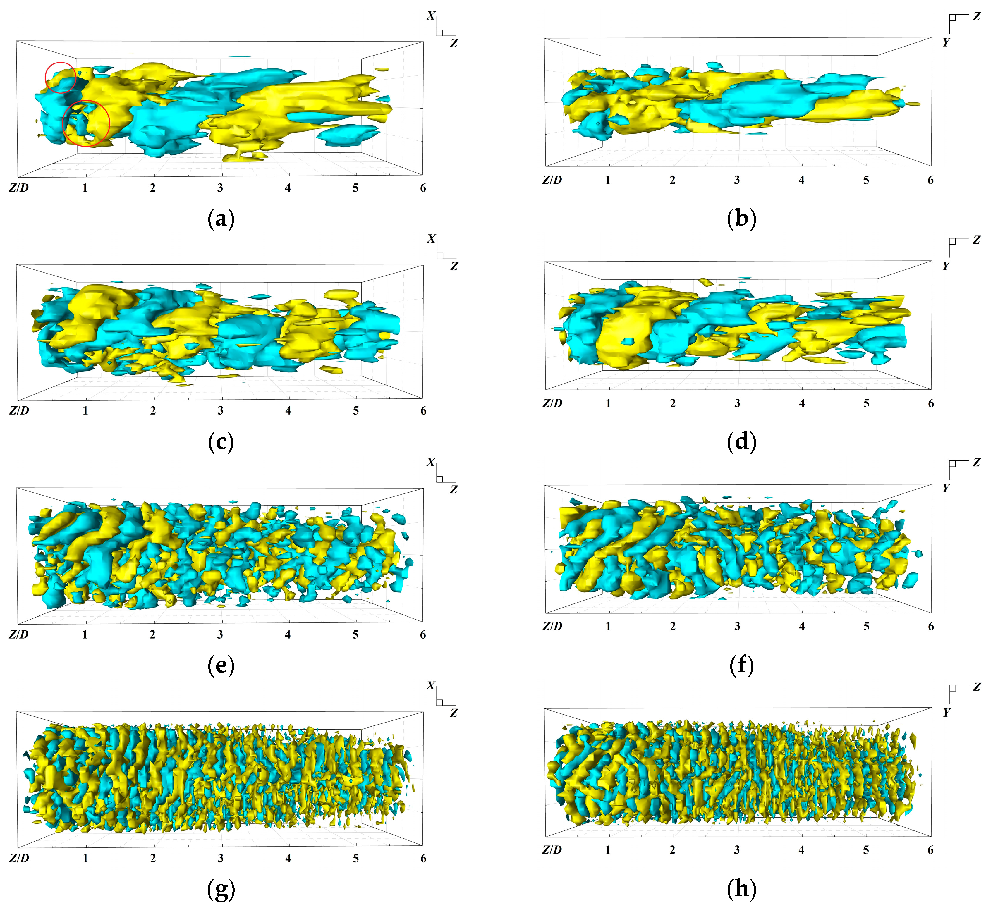
After carrying out the proper orthogonal decomposition, the coherent vortex structures of fluctuating modes were shown. The velocities of the iso-surfaces of the coherent vortex of the wake flow exhibited an annular trend in terms of circumferential connection. The annular structures formed by the coherent vortex gradually became more fragmented, and the number of structures increased as the mode order increased;

(3)

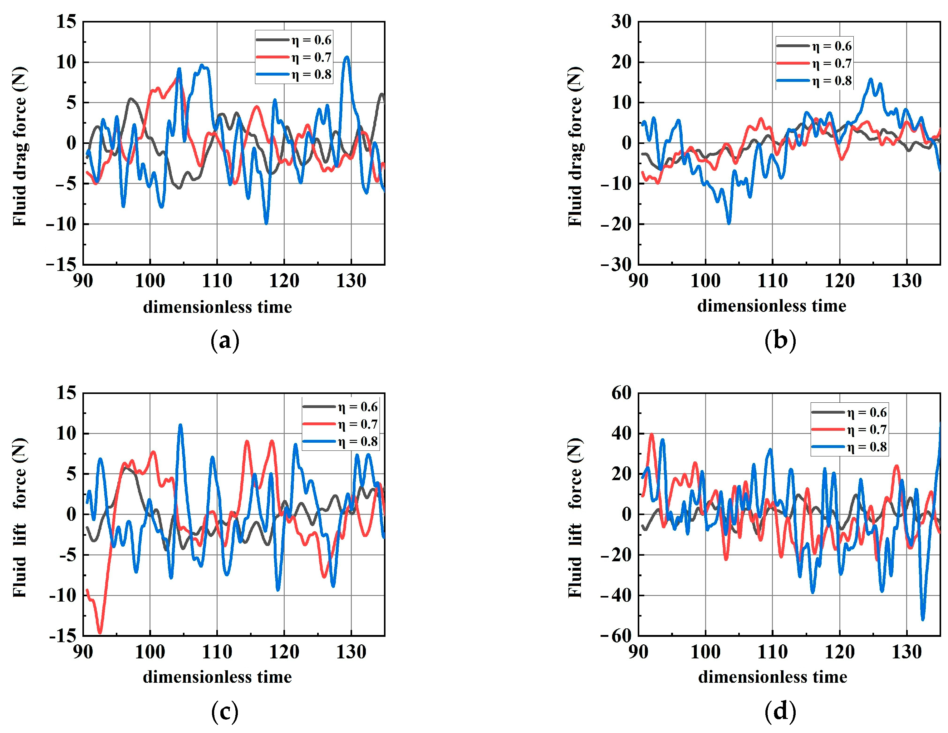
The steady component and transient component of hydrodynamic force were resolved, and the general trend seen in the forces in the transient components was that the maximum amplitude of forces reduced with the increase in mode order. The amplitude-, direction-, and time-dependent variations in the transient components constituted the transient evolution of the transient components in the hydrodynamic force. Using short-term Fourier transform, the frequency components and their variations in different terms across the whole time range can be acquired.

The transient model used in this study provided a perspective from which to build the connection between the flow structures and the hydrodynamic force. Using the transient model, the transient component of hydrodynamic force can be explained as the fluctuation of coherent vortex structures. Moreover, this model can provide evidence for the relation between the energy consumption of capsule motion and the spatial–temporal characteristic of the flow structure.

References

1. Balazadeh Meresht, N.; Moghadasi, S.; Munshi, S.; Shahbakhti, M.; McTaggart-Cowan, G. Advances in Vehicle and Powertrain Efficiency of Long-Haul Commercial Vehicles: A Review. Energies 2023, 16, 6809. [Google Scholar] [CrossRef]
2. Khazini, L.; Kalajahi, M.J.; Blond, N. An Analysis of Emission Reduction Strategy for Light and Heavy-Duty Vehicles Pollutions in High Spatial-Temporal Resolution and Emission. Environ. Sci. Pollut. Res. 2022, 29, 23419–23435. [Google Scholar] [CrossRef] [PubMed]
3. Achuo, E.D.; Miamo, C.W.; Nchofoung, T.N. Energy consumption and environmental sustainability: What lessons for posterity? Energy Rep. 2022, 8, 12491–12502. [Google Scholar] [CrossRef]
4. Xue, P.; Liu, J.; Liu, B.; Zhu, C. Impact of Urbanisation on the Spatial and Temporal Evolution of Carbon Emissions and the Potential for Emission Reduction in a Dual-Carbon Reduction Context. Sustainability 2023, 15, 4715. [Google Scholar] [CrossRef]
5. Javanmardi, E.; Hoque, M.; Tauheed, A.; Umar, M. Evaluating the Factors Affecting Electric Vehicles Adoption Considering the Sustainable Development Level. World Electr. Veh. J. 2023, 14, 120. [Google Scholar] [CrossRef]
6. Okyere, S.; Yang, J.; Adams, C.A. Optimizing the Sustainable Multimodal Freight Transport and Logistics System Based on the Genetic Algorithm. Sustainability 2022, 14, 11577. [Google Scholar] [CrossRef]
7. Shi, H.; Yuan, J.; Li, Y. The Impact of Swirls on Slurry Flows in Horizontal Pipelines. J. Mar. Sci. Eng. 2021, 9, 1201. [Google Scholar] [CrossRef]
8. Chen, Y.; Li, G.; Duan, J.; Liu, H.; Xu, S.; Guo, Y.; Hua, W.; Jiang, J. Review of Oil–Water Flow Characteristics of Emptying by Water Displacing Oil in Mobile Pipelines. Energies 2023, 16, 2174. [Google Scholar] [CrossRef]
9. Jiwa, M.Z.; Kim, Y.T.; Mustaffa, Z.; Kim, S.; Kim, D.K. A Simplified Approach for Predicting Bend Radius in HDPE Pipelines during Offshore Installation. J. Mar. Sci. Eng. 2023, 11, 2032. [Google Scholar] [CrossRef]
10. Hong, X.; Huang, L.; Gong, S.; Xiao, G. Shedding Damage Detection of Metal Underwater Pipeline External Anticorrosive Coating by Ultrasonic Imaging Based on HOG + SVM. J. Mar. Sci. Eng. 2021, 9, 364. [Google Scholar] [CrossRef]
11. Li, Z.; Wang, G.; Yao, S.; Yun, F.; Jia, P.; Li, C.; Wang, L. A Semi-Analytical Method for the Sealing Performance Prediction of Subsea Pipeline Compression Connector. J. Mar. Sci. Eng. 2023, 11, 854. [Google Scholar] [CrossRef]
12. Paul, A.R.; Bhattacharyya, S. Analysis and Design for Hydraulic Pipeline Carrying Capsule Train. J. Pipeline Syst. Eng. Pract. 2021, 12, 04021003. [Google Scholar] [CrossRef]
13. Asim, T.; Algadi, A.; Mishra, R. Effect of Capsule Shape on Hydrodynamic Characteristics and Optimal Design of Hydraulic Capsule Pipelines. J. Petrol. Sci. Eng. 2018, 161, 290–408. [Google Scholar] [CrossRef]
14. Asim, T.; Mishra, R.; Abushaala, S.; Jain, A. Development of A Design Methodology for Hydraulic Pipelines Carrying Rectangular Capsules. Int. J. Pres. Pip. 2016, 146, 111–128. [Google Scholar] [CrossRef]
15. Ulusarslan, D. Comparison of Experimental Pressure Gradient and Experimental Relationships for the Low Density Spherical Capsule Train with Slurry Flow Relationships. Powder Technol. 2008, 185, 170–175. [Google Scholar] [CrossRef]
16. O’Connell, R.; Lenau, C.; Zhao, T. Capsule Separation by Linear Induction Motor in Pneumatic Capsule Pipeline Capsule Transport System. J. Pipeline Syst. Eng. 2010, 1, 84–90. [Google Scholar] [CrossRef]
17. Chen, Y.; Guo, D.; Chen, Z.; Fan, Y.; Li, X. Using a Multi-Objective Programming Model to Validate Feasibility of an Underground Freight Transportation System for the Yangshan Port in Shanghai. Tunn. Undergr. Space Technol. 2018, 81, 463–471. [Google Scholar] [CrossRef]
18. Asim, T.; Mishra, R. Computational Fluid Dynamics Based Optimal Design of Hydraulic Capsule Pipelines Transporting Cylindrical Capsules. Powder Technol. 2016, 295, 180–201. [Google Scholar] [CrossRef]
19. Liu, H.; Graze, H. Lift and Drag on Stationary Capsule in Pipeline. J. Hydraul. Eng. ASCE 1983, 109, 28–47. [Google Scholar] [CrossRef]
20. Asim, T.; Mishra, R. Optimal Design of Hydraulic Capsule Pipelines Transporting Spherical Capsules. Can. J. Chem. Eng. 2016, 94, 966–979. [Google Scholar] [CrossRef]
21. Zhao, Y.; Li, Y.; Song, X. PIV Measurement and Proper Orthogonal Decomposition Analysis of Annular Gap Flow of a Hydraulic Machine. Machines 2022, 10, 645. [Google Scholar] [CrossRef]
22. Vooren, J. The Downstream Flow of a Transonic Aircraft: A Small Disturbance, High Reynolds Number Analysis. Aerosp. Sci. Technol. 2008, 12, 457–468. [Google Scholar] [CrossRef]
23. Aono, H.; Liang, F.; Liu, H. Near and Far-Field Aerodynamics in Insect Hovering Flight: An Integrated Computational Study. J. Exp. Biol. 2008, 211, 239–257. [Google Scholar] [CrossRef] [PubMed]
24. Chen, Z.; Zhang, B. Drag Prediction Method Investigation Basing on the Wake Integral. Acta Aerodyn. Sin. 2009, 27, 329–334. [Google Scholar] [CrossRef]
25. Paparone, L.; Tognaccini, R. Computational Fluid Dynamics-Based Drag Prediction and Decomposition. AIAA J. 2012, 41, 1647–1657. [Google Scholar] [CrossRef]
26. Talezade, A.; Mojtaba, S.; Manshadi, D. Streamlined Bodies Drag Force Estimation Using Wake Integration Technique. J. Braz. Soc. Mech. Sci. 2020, 42, 293. [Google Scholar] [CrossRef]
27. Lumley, J.; Blossey, P. Control of Turbulence. Annu. Rev. Fluid Mech. 1998, 30, 311–327. [Google Scholar] [CrossRef]
28. D’Agostino, D.; Diez, M.; Felli, M.; Serani, A. PIV Snapshot Clustering Reveals the Dual Deterministic and Chaotic Nature of Propeller Wakes at Macro- and Micro-Scales. J. Mar. Sci. Eng. 2023, 11, 1220. [Google Scholar] [CrossRef]
29. Zhao, Y.; Li, Y.; Sun, X. Modal Analysis of the Hydrodynamic Force of a Capsule in a Hydraulic Capsule Pipeline. J. Mar. Sci. Eng. 2023, 11, 1738. [Google Scholar] [CrossRef]
Figure 1. Schematic of the control volume.
Sustainability 15 15575 g001
Figure 2. (a) The schematic of physical experimental devices. (b) The schematic of the capsule.
Sustainability 15 15575 g002
Figure 3. The physical experimental schematic of the scaled model for an HCP system. (The red box contains the measuring devices).
Sustainability 15 15575 g003
Figure 4. The schematic of the calculation domain.
Sustainability 15 15575 g004
Figure 5. The coherent structure contoured by the iso-surface of velocity in the wake flow, with yellow iso-surface U/(|Umax|) = 0.2 and indigo iso-surface U/(|Umax|) = −0.2: (a) XOZ view of mode 1; (b) YOZ view of mode 1; (c) XOZ view of mode 5; (d) YOZ view of mode 5; (e) XOZ view of mode 20; (f) YOZ view of mode 20; (g) XOZ view of mode 50; (h) YOZ view of mode 50. (The red circles marked the merging of multiple bundles of iso-surface structures).
Sustainability 15 15575 g005
Figure 6. The transient component of the hydrodynamic force corresponding to fluctuating modes: (a) fluid drag force of Q = 40 m3 h−1; (b) fluid drag force of Q = 60 m3 h−1; (c) fluid lift force of Q = 40 m3 h−1; (d) fluid lift force of Q = 60 m3 h−1.
Sustainability 15 15575 g006
Figure 7. The transient component of the hydrodynamic forces in the time range: (a) fluid drag force of Q = 40 m3 h−1; (b) fluid drag force of Q = 60 m3 h−1; (c) fluid lift force of Q = 40 m3 h−1; (d) fluid lift force of Q = 60 m3 h−1.
Sustainability 15 15575 g007
Figure 8. The power spectrum density maps of time coefficients corresponding to the fluid drag force of the typical modes given by short-term Fourier transform: (a) PSD map of mode 1; (b) PSD map of mode 5; (c) PSD map of mode 16; (d) PSD map of mode 17; (e) PSD map of mode 40; (f) PSD map of mode 46.
Sustainability 15 15575 g008