Photovoltaic/Hydrokinetic/Hydrogen Energy System Sizing Considering Uncertainty: A Stochastic Approach Using Two-Point Estimate Method and Improved Gradient-Based Optimizer

Abstract

In this paper, stochastic sizing of a stand-alone Photovoltaic/Hydrokinetic/Hydrogen storage energy system is performed with aim of minimizing the cost of project life span (COPL) and satisfying the reliability index as probability of load shortage (POLS). The stochastic sizing is implemented using a novel framework considering two-point estimate method (2m+1 PEM) and improved gradient-based optimizer (IGBO). The 2m+1 PEM is used to evaluate the impact of uncertainties of energy resource generation and system demand on sizing problem. The 2m+1 PEM utilizes the approximate method to account for these uncertainties. In order to avoid premature convergence, the gradient-based optimizer (GBO), a meta-heuristic algorithm influenced by Newtonian concepts, is enhanced using a dynamic lens-imaging learning approach. The size of the system devices, which is determined utilizing the IGBO with the COPL minimization and optimally satisfying the POLS, is one of the optimization variables. The results of three hPV/HKT/FC, hPV/FC, and hHKT/FC configurations of the system are presented in two situations of deterministic and stochastic sizing without and with taking uncertainty into consideration. The findings showed that the hPV/HKT/FC configuration and the IGBO performed better than other configurations and techniques like conventional GBO, particle swarm optimization (PSO), and artificial electric field algorithm (AEFA) to achieve the lowest COPL and POLS (higher reliability) in various cases. Additionally, the COPL for the hPV/HKT/FC, hPV/FC, and hHKT/FC configurations increased by 7.63%, 7.57%, and 7.65%, respectively, while the POLS fell by 5.01%, 4.48%, and 4.59%, respectively, contrasted to the deterministic sizing, according to the results of stochastic sizing based on 2m+1 PEM. As a result, the findings indicate that in the deterministic sizing model, the quantity of output and energy storage is insufficient to meet demand under unknown circumstances. Applying stochastic sizing while taking into account the volatility of both supply and demand can, therefore, be an economically sound way to meet demand.

1. Introduction

1.1. Motivation and Background

In the past few decades, the usage of renewable energy has become more widespread. Several nations are attempting to make money off of these resources due to their industrial usage and geographic location. The rising cost of fossil fuels and the negative environmental effects of these resources are two factors driving more countries to the application of renewable energy resources (RES) [1,2]. Distributed generation (DG) according to the RES is advocated for stand-alone areausage to reduce the cost of installing electricity transmission lines. Saving money is one of the main objectives when utilizing renewable sources of energy [3,4]. A clever way to lower the network’s economic growth and building costs is to meet the energy needs of remote loads with sustainable resources [5,6]. By integrating two or more RES with storage technology, hybrid power plants can control changes in energy output, boosting load reliability [7,8]. In addition, one of the renewable energy sources that have recently received much attention is hydrokinetic turbine technology (HKT), which has evolved from wind turbine technology, which consists of several large axial flow turbines similar to underwater wind turbines. There is also considerable interest in the potential of small hydrokinetic turbines to generate off-grid electricity from rivers [9,10]. Crooks et al. (2022) presented the computational design of a hydrokinetic horizontal parallel stream direct-drive in [9], Kirke (2020) addressed the challenge of providing small scale electrical power and pumping from rivers in [10], and Saini and Saini (2023) evaluated the clearance and blockage impacts on the hydrodynamic performance of hybrid hydrokinetic turbines. These clean energy resources can be used in hybrid energy systems along with other energy sources [11]. The demand reliability of the hybrid RES (HRES) is increased through the addition of a storage system. Consequently, it plays a significant part in the reliable design of hybrid systems. Batteries and hydrogen-based fuel cells are two of the more important substantial technologies for storing energy available today [12,13]. Fuel cells are a long-term preservation method that utilizes hydrogen storage, whereas batteries are a short-term storage device. However, research on the development of HRESs has revealed that the cost of developing HRESs that utilize hydrogen is significantly higher than developing HRESs depending on battery storage [14]. The two operating modes for hybrid energy systems are autonomous and non-autonomous. In their autonomous configuration, these systems have no power exchange with the network, and the storage system plays a crucial role in continual load supply, boosting reliability, and lowering the cost of production [15]. The HRES may both inject electricity into the network and receive power from it when it becomes linked to the grid. As a result, receiving and injecting electricity might change system design characteristics. Furthermore, in HRES, the sizing process has a big impact on how accurate the design outcomes are [16]. Decreasing the price of producing electricity via the HRES, which is provided as the design’s economic measure, is a particularly popular objective function. One of the key concerns in the sizing of HRESs is reliability assessment, which expresses reliability constraints as a technical assessment [17]. To fulfill the reliability limitation and reduce the cost of energy production, the size of the HRES elements according to the economic and technical metrics would be calculated [18,19]. On the other hand, the uncertainty of renewable energy sources is another challenge facing these systems in meeting load demand. In other words, in such systems, the reserve energy level is one of the uncertain parameters in effective uncertainty conditions [20,21]. For the purpose of determining the ideal sizing of system elements with high computation and optimization capabilities, HRES engineers have paid a lot of attention lately to the application of cognitive and optimization iteration approaches.

1.2. Literature Review and Research Gaps

Several studies are conducted in previous studies on sizing of the HRESs, energy storage system, sizing criteria, and optimization technique. In [22], sizing of an hPV/WT/Biowaste combined with a hydro-pumped storage system is performed to mitigate the cost of energy (COE). Jin and Yang (2023) presented sizing of hybrid entirely electric ships in [23] while considering connected optimal energy management and voyage planning for minimizing the total cost by means of mixed-integer nonlinear programming (MINLP). Ghoniem et al. (2023) developed the sizing of an hPV/FC system in [24] via the HOMER by minimizing the COE and the net present cost. Mohammed (2023) performed designing a PV/FC system to reduce overall life-cycle expenses for a renewable farm via the MINLP in [25]. The off-grid hPV/WT system with battery is given in [26] with the COE minimized and the possibility of unfulfilled demand satisfied using the firefly algorithm (FA). In [27], multi-objective optimization of an hPV/WT/Battery system is presented t to minimize the cost of energy for Brazilian cities considering economic viability. Choosing WTs assuming the maximum permitted size limit with the goal of minimizing loss and voltage characteristics enhanced. The study conducted in [28] examines the allocation and sizing of WTs in the network using an improved spotted hyena optimizer (ISHO). An hPV/WT/Battery system sizing is presented via improved search space reduction algorithm to minimize the cost of energy considering Effect of adding electric vehicles in [29]. To optimize the power output of PV units and prevent power waste and potential instability resulting from inadequate PV power via conventional droop control, [30] suggests an enhanced droop control method. Jahannoosh and Nowdeh (2020) developed design of an hPV/WT/FC system with minimizing the energy costs and fulfillment of reliability constraints through the utilization of an enhanced sine–cosine algorithm (ISCA) according to [31]. In [32], sizing of an hPV/WT/Battery system for buildings supply is performed via a multi objective NSGA-II to minimize the total energy transfer and satisfying the reliability constraints. The sizing of a hPV/FC system is investigated in [33] minimizing the life cycle cost while ensuring the satisfaction of the LPSP via a harmony search algorithm (HSA). In [34], sizing of an hPV/Battery system is performed utilizing salp swarm optimization (SSO) with minimization of life-cycle cost considering the LPSP. Naderipour et al. (2022) presented an artificial electric field algorithm (AEFA) for designing an hPV/WT/Battery system for providing the load with the system cost minimization in [35]. Samy et al. (2019) developed the sizing of a hPV/FC system with cost minimization and satisfying the LPSP using the FPA in [36]. In [37], an hPV/WT/FC system sizing is conducted with the aim of overall system cost minimization through the utilization of the PSO. A sizing structure for a hPV/WT/Biowaste system is performed by minimizing the life cycle costs using a genetic algorithm (GA) in [38]. Gharibi and Askarzadeh (2019), implemented the design of an hPV/FC/Diesel system to minimize the cost while ensuring the LPSP using a crow search algorithm according to [39]. The optimum hPV/Battery with super capacitor energy storage system sizing technique is suggested via a based-on-rules algorithm with minimizing annual system operational cost by Yang et al. (2023) in [40]. Liu et al. (2023) developed an enhanced artificial ecosystem-based optimization algorithm (IAEO) to size an hPV/FC system in order to reduce the energy cost whereas satisfying the reliability requirement according to [41]. Naderipour et al. (2021) performed an hPV/HKT/FC energy system optimally to minimize the COE via the whale optimization algorithm (WOA) according to [42].

Table 1. Summary of the literature review.

Ref.	Configuration	HKT	Cost	Reliability	Uncertainty	Improved Solver
[22]	PV + WT + Biowaste	No	Yes	Yes	No	No
[23]	FC + Battery	No	Yes	No	No	No
[24]	PV + Battery + Diesel	No	Yes	Yes	No	No
[25]	PV + FC	No	Yes	Yes	No	No
[26]	PV + WT + Battery	No	Yes	Yes	No	No
[27]	PV + WT + Battery	No	Yes	Yes	No	No
[28]	WT	No	No	No	Yes	Yes
[29]	PV + WT + Battery	No	Yes	Yes	No	Yes
[30]	PV	No	No	No	Yes	No
[31]	PV + WT + Fuel cell	No	Yes	Yes	No	No
[32]	PV + WT + Battery	No	Yes	Yes	No	No
[33]	PV + Fuel cell	No	Yes	Yes	No	No
[34]	PV + Battery	No	Yes	Yes	No	No
[35]	PV + WT + Battery	No	Yes	Yes	No	No
[36]	PV + Fuel cell	No	Yes	Yes	No	No
[37]	PV + WT + Battery	No	Yes	Yes	No	No
[38]	PV + WT + Biowaste	No	Yes	No	No	No
[39]	PV + Fuel cell + Diesel	No	Yes	Yes	No	No
[40]	PV + Battery	No	Yes	No	No	No
[41]	PV + WT + FC	No	Yes	Yes	No	Yes
[42]	PV + WT + HKT	Yes	Yes	Yes	No	No
This paper	PV + WT + HKT	Yes	Yes	Yes	Yes	Yes

presents a summarized review of the background research.

The following are the research gaps in the size of hybrid energy systems as indicated by the literature review and Table 1:

• Battery storage, in particular, was used in the majority of research [22,23,24,25,26,27,28,29,30,31,32,33,34,35,36,37,38,39,40,41] on the size of HRESs made up of solar and wind sources to fulfill the demand. Hydrokinetic (HKT) energy systems have recently been considered in order to improve the effectiveness of power generation sources. As a result, the inclusion of HKT resources in the HRES may improve energy efficiency.
• The majority of hybrid energy system sizing studies, such those in [22,23,24,25,26,27,28,29,30,31,32,33,34,35,36,37,38,39,40], have not taken modeling uncertainty into account when determining system sizes. Keep in mind that the RES’s capacity and production are unclear. Therefore, in one scenario, the amount of load or renewable generation could be more or less than what the deterministic model predicted. The results from the stochastic sizing are less reliable than those from the deterministic model in this example because the quantity of batteries selected in the deterministic model could not be sufficient to account for the variations in load demand and renewable resource generation.
• Due to the enormous number of scenarios it takes into account, the Monte Carlo simulation (MCS) method, one of the standard approaches to uncertainty modeling, has a very high computational cost and necessitates the employment of scenarios reduction techniques. Additionally, the probability distribution function (PDF) of its inputs has a significant impact on the outcome.
• One of the most crucial elements in finding the best solution for the sizing of HRESs is the employment of robust and highly accurate optimization algorithms. According to the literature, in a small number of studies, the effectiveness of these algorithms is improved to avoid premature convergence, the risk that these methods may become stuck solving challenging problems at the local optimal level, and the possibility that increasing their efficiency may lead to rapid convergence to the optimal solution with low tolerance.

1.3. Contributions

The following list of research gaps in HRES scaling with various generation units and storage systems is based on the study background and Table 1:

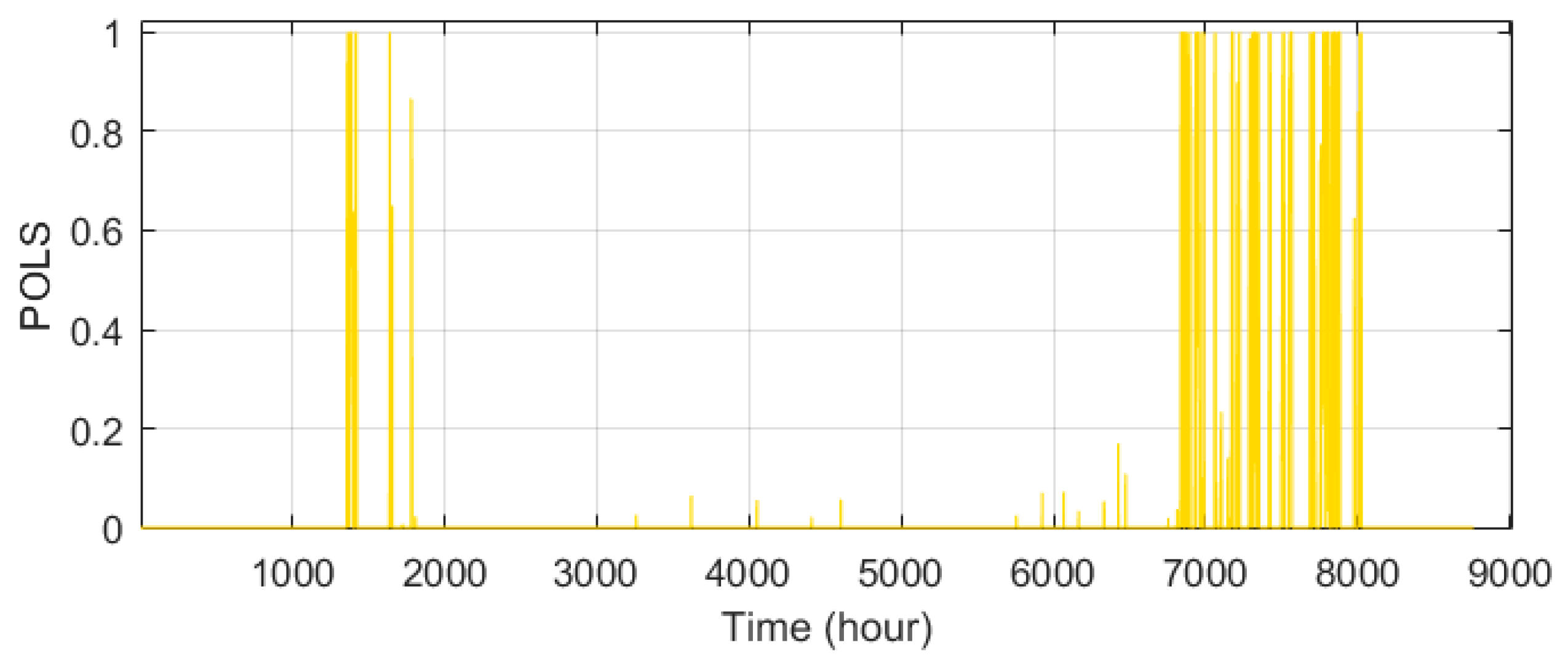
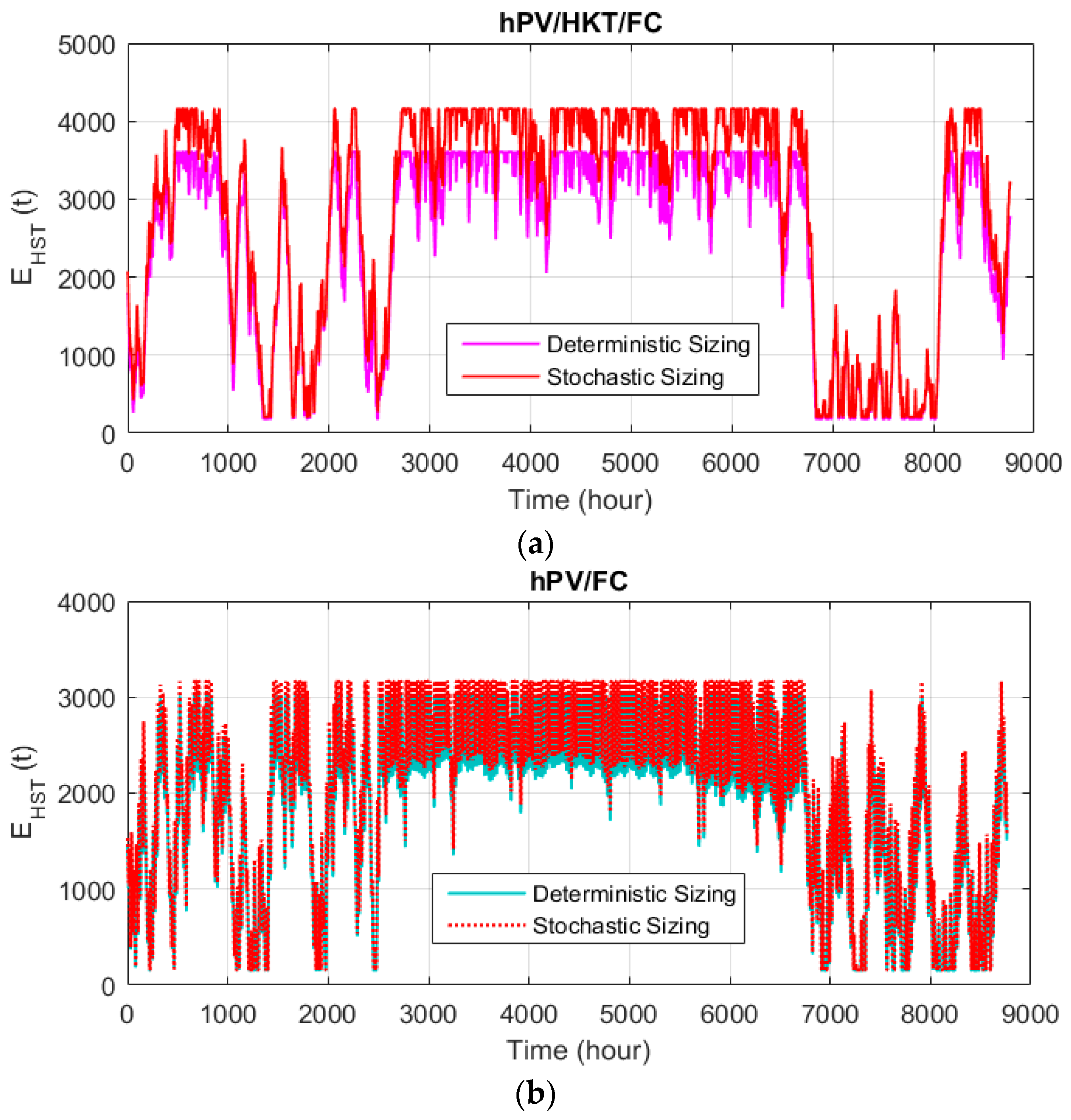
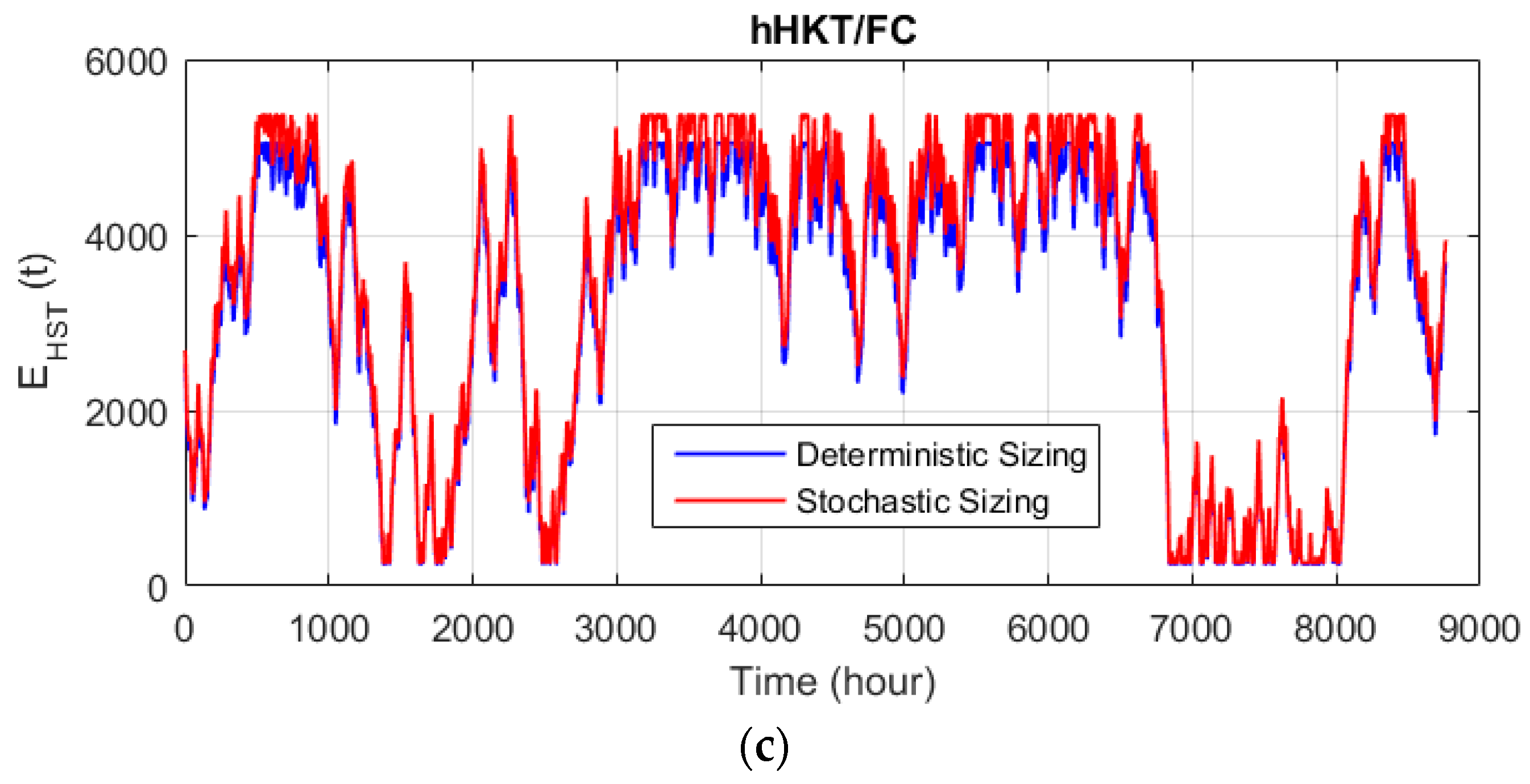
• Stochastic sizing of a stand-alone hybrid photovoltaic/hydrokinetic/fuel cell energy system (hPV/HKT/FC) integrated with hydrogen storage is carried out in this study with the goal of minimizing the cost of project life span (COPL) and the reliability index as the probability of load shortage (POLS), while taking into account the unpredictability of renewable resource generation and system demand.
• In order to properly express and analyze uncertainties, the 2m+1 PEM [43,44] is used to describe the uncertainties of RES generation and system load demand. The 2m+1 PEM does not rely on the PDF of unknown variables, in contrast to the MCS. Instead, it makes use of the original statistical moments to solve the approximations’ inadequacies. Additionally, it shows a lower computing burden and quicker iteration convergence as compared to the MCS. The simulation results are shown for three hPV/HKT/FC, hPV/FC, and hHKT/FC configurations of the HRES in two situations of deterministic and stochastic sizing, with and without taking uncertainty into account.
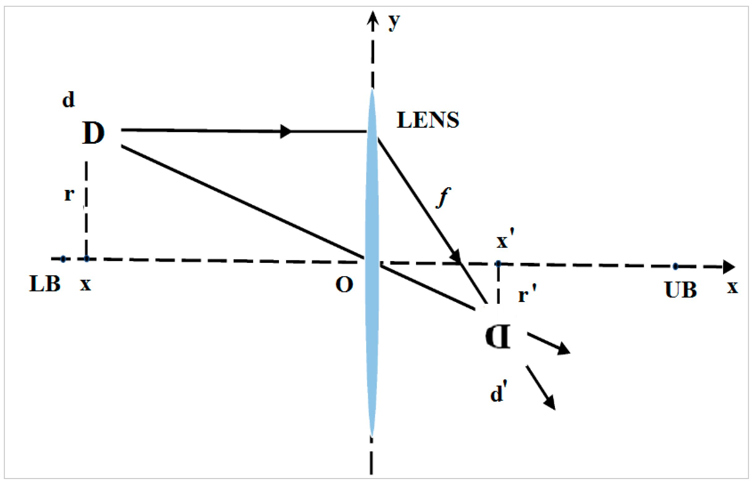
• The GBO [45] is a meta-heuristic algorithm for solving mathematical problems that draws its inspiration from Newton’s method and is enhanced by a dynamic lens-imaging learning method to avoid premature convergence. The IGBO is used to determine the decision variables, such as the HRES components’ ideal capacity.
• The suggested methodology is compared to other approaches, including traditional GBO, particle swarm optimization (PSO) [46], artificial electric field algorithm (AEFA) [47], and earlier works, to demonstrate its superiority.

1.4. Paper Structure

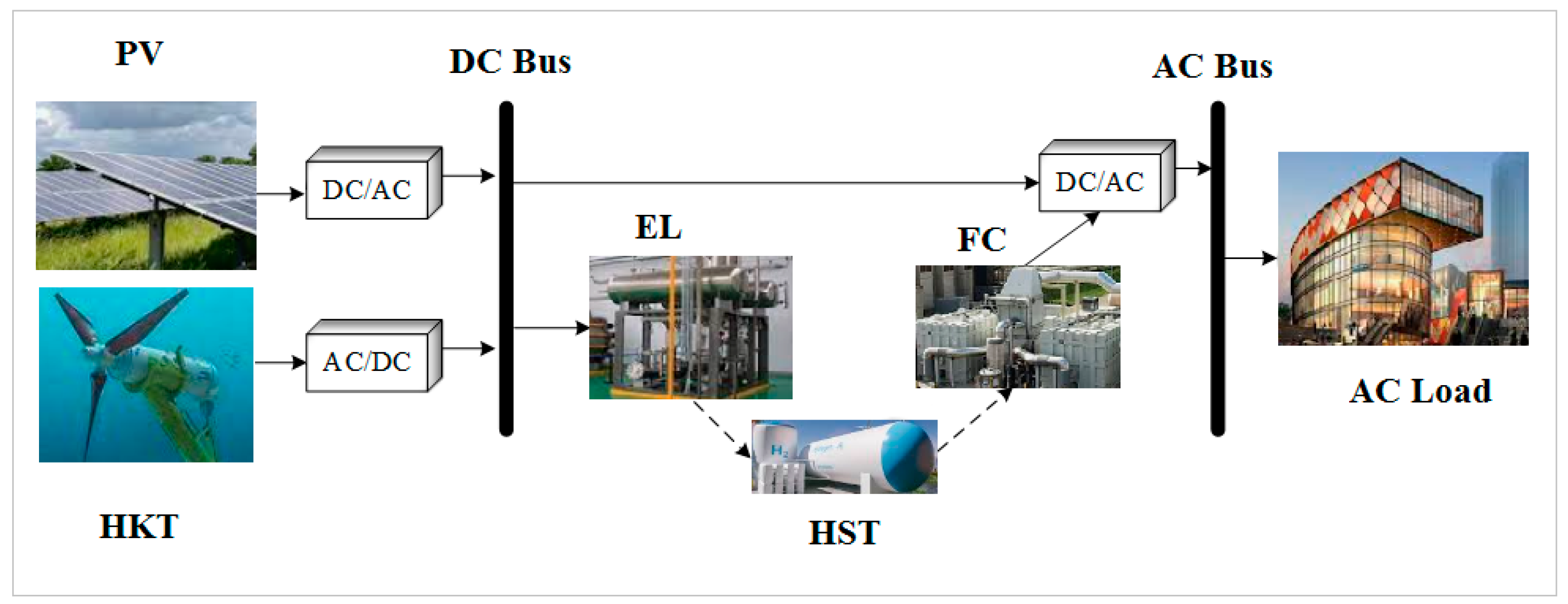
This paper comprises the sections listed below. In Section 2, the configurations, models, and operations of hybrid energy systems are described. Section 3 describes the 2m+1 PEM used to model uncertainty in stochastic sizing problems. In Section 4, the optimization methodology is outlined as well as the conventional GBO, improved GBO (IGBO), and its applicability to the sizing problem. Section 5 provides the results and in Section 6, the findings are summarized.

2. The Studied HRES

2.1. Configurations

In the broadest sense, the HRES is the one that integrates and exploits multiple easily accessible sources. The studied HRES comprises two renewable energy components, including PVs and HKTs, which are incorporated with a fuel cell stack comprising an electrolyzer (EL), a hydrogen storage tank (HST), and a fuel cell (FC). Before the process of optimum sizing, mathematical modeling of the HRES is a necessary prerequisite. The configuration and modeling of the HRES components are outlined in detail in the following section. The HRES configuration is illustrated in Figure 1. PVs and HKTs are the main types of electricity production applied to meet electricity demand. The execution of a load-following strategy is viewed as a successful approach to handling energy within this system. The load-following strategy is an approach used for efficiently overseeing renewable generation units to satisfy the hourly load demand. Utilizing the RES to satisfy the system’s capacity requirements is the first step in this specific approach. Utilizing a fuel cell system based on hydrogen storage, the excess power from renewable units is injected into the electrolyzer to produce hydrogen. In addition, if there is a shortage of load, hydrogen is transferred into the fuel cell in order to generate electricity, which is then transferred to the load through an inverter. In instances where renewable sources and fuel cells cannot meet the load, a portion of the load is eliminated.

2.2. The HRES Modelling

2.2.1. PV

The calculation of PV power is determined by the solar radiation that is incident upon the surface of the panel, as stated by [27,30,31].

$$P_{PV}=\frac{{(P}_{PV,Nominal}\times {\mathrm{E}\mathrm{t}\mathrm{t}\mathrm{a}}_{PV})\times ({Sol}_{VER}\left(t\right)\times \cos \left({\theta }_{PV}\right)+{Sol}_{HOR}(t)\times \sin ({\theta }_{PV}))}{{Sol}_{REF}}$$

(1)

where ${Sol}_{VER}\left(t\right)$ and ${Sol}_{HOR}\left(t\right)$ denote the vertical and horizontal irradiance components, respectively. ${Sol}_{REF}$ denotes irradiance under standard conditions (1000 W/m²). The parameter ${\theta }_{PV}$ represents the angle of PV installation in degrees. ${\mathrm{E}\mathrm{t}\mathrm{t}\mathrm{a}}_{PV}$ corresponds to the efficiency of PV tracking, and $P_{PV,Nominal}$ stands for the nominal power of the PV system.

2.2.2. HKT

Because the efficacy of HKT systems is comparable to that of hydropower plants, their use has increased and expanded. The HKT current flow is utilized to generate electricity. This investigation employs horizontal axis turbines. The HKT-provided power is estimated by factoring in a cut-in, cut-out, and rated water flow by [48]

$$P_{HKT=}\left\{\begin{array}{c}0;V_{HKT}\le V_{HKTcutin},V_{HKT}\ge V_{HKTcutout}\\ 0.5\delta A{C}_P{V_{HKT}}^3; V_{HKTcutin}<V_{HKT}<V_{HKTr}\\ P_{HKTr}; V_{HKTr}\le V_{HKT}\le V_{HKTcutout}\end{array}\right.$$

(2)

where $P_{HKT}$ and $P_{HKTr}$ refer to the HKT power and its nominal power (kW), respectively; $V_{HKT}$ denotes water current speed, $V_{HKTcutin}$ indicates the cut-in speed, $V_{HKTr}$ is the nominal speed, and $V_{HKTcutout}$ refers to the cutout speed (m/s). $\delta$ is the density of fluid (kg/m²), $A$ denotes the area of cross-sectional turbine (m²), and $C_P$ clears the coefficient of power.

2.2.3. EL

The EL generates both hydrogen and oxygen through the electrolysis of water. In the event of an HRES power deficit, the hydrogen stored in the HS cylinder will be sent to the FC to compensate for the demand [27,30,31].

$$P_{\mathrm{E}\mathrm{L} \mathrm{t}\mathrm{o} \mathrm{H}\mathrm{S}\mathrm{T}}=P_{HST-EL}\times {Etta}_{EL}$$

(3)

where ${Etta}_{EL}$ is the EL proficiency, and $P_{HST-EL}$ is the transferred power to the EL via the HKT, and PV sources.

2.2.4. HST

Hydrogen is stored under high pressure in an HST. The HST energy is achieved by [27,30,31]

$$E_{HST}\left(t\right)=E_{HST}(t-1)+P_{\mathrm{EL} \mathrm{to} \mathrm{HST}}\left(t\right)\times \mathsf{\Delta }t-{\mathrm{P}}_{\mathrm{H}\mathrm{S}\mathrm{T}-\mathrm{F}\mathrm{C}}\left(t\right)\times \mathsf{\Delta }t\times {Etta}_{HST}$$

(4)

where $E_{HST}(t-1)$ is HST energy in t − 1, $P_{\mathrm{E}\mathrm{L} \mathrm{t}\mathrm{o} \mathrm{H}\mathrm{S}\mathrm{T}}$ is power of the EL sent to the HST, ${\mathrm{P}}_{\mathrm{H}\mathrm{S}\mathrm{T}-\mathrm{F}\mathrm{C}}$ denotes power of HST sent to the FC. Additionally, $E_{HST}\left(t\right)={HHV}_{H2}{\times m}_{HST}\left(t\right)$ that $m_{HST}\left(t\right)$ is H₂ mass (kg) at time t, ${HHV}_{H2}$ clear the value of hydrogen heating, and ${Etta}_{HST}$ is the HST proficiency.

2.2.5. FC

The power generated by the FC is computed by the hydrogen gained, and its equation is therefore defined by

$$P_{FC-INV}=P_{HST-FC}\times {Etta}_{FC}$$

(5)

where ${EF}_{FC}$ is the FC efficiency.

2.2.6. Inverter

The inverter injects the following power formula into the load:

$$P_{Inv-Load}=(P_{FC-Inv}+P_{HRES-Inv})\times {Etta}_{Inv}$$

(6)

here, ${Etta}_{Inv}$ is the inverter efficiency, and $P_{HRES-Inv}$ is the HRES power transferred to the inverter.

3. Stochastic Approach

This study focuses on the stochastic scheduling of an HRES. The main challenge addressed in this study is the uncertainty associated with RESs generation and load demand. There are three distinct groups that encompass uncertainty modeling methods such as Monte Carlo simulation (MCS), as well as analytical, and approximate techniques. This study employs the 2m+1 PEM approach, utilizing approximate approaches to effectively represent and analyze uncertainties [43,44]. In contrast to the MCS, the PEM does not rely on the probability density function (PDF) of uncertain variables. Instead, it addresses the limitations associated with the approximations by utilizing the initial statistical moments. Furthermore, in comparison to the MCS, it exhibits a reduced computational burden and faster convergence in terms of iterations. The 2m+1 PEM is derived using statistical data, specifically the low estimated value obtained from the central moments (CMs) related to the random input variables (RIVs) [43,44]. The statistical moments related to the output variables are determined by evaluating the objective function 2m+1 times while considering only the two CMs for each RIV. In the context of the PEM framework, the CMs are utilized to identify representative points, referred to as centers, for each variable. The model is solved using representative points, and the statistical information of the uncertain output variable is determined based on the answers derived from these representative points [45,46,47]. To ascertain the CMs of the output variables pertaining to the stochastic sizing problem, the procedural guidelines for the application of the 2m+1 PEM are outlined as follows:

Step (1)

Define the quantity of the RIV (m).

Step (2)

Specify the moment vector of the output variable as $E(U^i)=0, i=1,2$. Here, $E(U^i)$ signifies the moment vector of the output variable at the ith position.

Step (3)

Tuning $c=1 (c=1,2,\mathrm{\dots },m)$.

Step (4)

The 2 standard positions of the variable randomly are acquired in the following manner:

$${\zeta }_{c,j}=\frac{{\lambda }_{c,3}}{2}+{(-1)}^{3-j}.\sqrt{{\lambda }_{c,4}-\frac{3{\lambda }_{{}_{c,3}}^2}{4}}j=1,2$$

(7)

where ${\zeta }_{c,j}$ denotes the standardized positions of the RIV, ${\lambda }_{c,3}$ represents the skewness of the RIVs $z_c$, and ${\lambda }_{c,4}$ signifies the expression for the kurtosis of the RIV.

Step (5)

The positions $z_c$ are delineated as follows:

$$z_{c,j}={\mu }_{z_c}+{\zeta }_{c,j}.{\sigma }_{z_c}j=1,2$$

(8)

where $z_{c,j}$ represents the positions of the RIVs, ${\mu }_{z_c}$ denotes the mean of $z_c$, and ${\sigma }_{z_c}$ signifies the standard deviation of $z_c$.

Step (6)

The deterministic sizing of the HRES is implemented for two locations.

$$U_{c,j}=f({\mu }_{z_1},{\mu }_{z_2},\mathrm{\dots },z_{c,j},\mathrm{\dots },{\mu }_{z_m})j=1,2.$$

(9)

here, $U_{c,j}$ denotes deterministic sizing for the specified positions $z_c$.

Step (7)

Two weighting factors ($g_{c,j}$) for $z_c$ are established:

$$g_{c,j}=\frac{{(-1)}^{3-j}}{{\zeta }_{c,j}.({\zeta }_{c,1}-{\zeta }_{c,2})}j=1,2.$$

(10)

Step (8)

Update $E(U^i)$.

$$E(U^i)=E(U^i)+{\displaystyle {\sum }_{j=1}^2{g}_{c,j}{(U_{c,j})}^i.}$$

(11)

Step (9)

Repeat Steps 4 to 8 for each subsequent iteration of the variable, until all RIVs have been taken into consideration.

Step (10)

The hPV/HKT/FC deterministic sizing problem is executed based on the RIV vector provided by

$$z_{\mu }=[{\mu }_{z_1},{\mu }_{z_2},\mathrm{\dots },{\mu }_{z,c},\mathrm{\dots },{\mu }_{z_m}]j=1,2.$$

(12)

here, $z_{\mu }$ represents the vector of RIVs.

Step (11)

The weight coefficient for the HRES sizing, which was solved in Step (10), is computed using the following formula.

$$g_0=1-{\displaystyle {\sum }_{c=1}^m\frac{1}{{\lambda }_{c,4}-{\lambda }_{c,3}^2}.}$$

(13)

where, $g_0$ represents the weighting factor associated with the HRES sizing problem.

Step (12)

$E(U^i)$ is outlined as follows.

$$E(U^i)={{\displaystyle {\sum }_{c=1}^m{\displaystyle {\sum }_{j=1}^2{g}_{c,j}[({\mu }_{z_1},{\mu }_{z_2},\mathrm{\dots },{\mu }_{c,j},\mathrm{\dots },{\mu }_{z_m})]}}}^i+g_0{[U(z_{\mu })]}^i.$$

(14)

Step (13)

According to the statistical moments related to the output random variable (ROV), the mean value ${\mu }_U$ and standard deviation ${\sigma }_U$ are established as follows.

$${\mu }_U=E(U);{\sigma }_U=\sqrt{E(U^2)-{\mu }_{{}_U}^2}.$$

(15)

In this context, ${\mu }_U$ and ${\sigma }_U$ denote the mean and standard deviation of the ROV, respectively.

4. Problem Formulation

In this section, the objective function of the HRES sizing problem and also the constraints are formulated in detail.

4.1. Objective Function

The objective function for the HRES sizing is defined as the cost of project life span (COPL) minimization for 20 years [22,37]. The COPL includes capital (${\partial }_{CAP}$), maintenance and operation (${\partial }_{MAINOP}$), and replacement (${\partial }_{REP}$) costs of the HRES [27,30,31]. The objective function and each of its parts are formulated in detail below:

$$Min COPL={\partial }_{CAP}+{\partial }_{MAINOP}+{\partial }_{REP}$$

(16)

$$\begin{gathered} { {\partial }_{CAP}=\partial }_{PVcap}\times {\mathsf{\varpi }}_{PV}+{\partial }_{HKTcap}\times {\mathsf{\varpi }}_{HKT}+{\partial }_{ELcap}\times {\mathsf{\varpi }}_{EL}+{\partial }_{HSTcap}\times {\mathsf{\varpi }}_{HST} \\ +{\partial }_{FCcap}\times {\mathsf{\varpi }}_{FC}+{\partial }_{Invcap}\times {\mathsf{\varpi }}_{Inv} \end{gathered}$$

(17)

$$\begin{gathered} {\partial }_{MAINOP}=\frac{{\left(1+\left(\kappa \right)\right)}^{\tau }-1}{\left(\kappa \right){\left(1+\left(\kappa \right)\right)}^{\tau }}\times ({\partial }_{PVmainop}\times {\mathsf{\varpi }}_{PV}+{\partial }_{HKTmainop}\times {\mathsf{\varpi }}_{HKT} \\ +{\partial }_{ELmainop}\times {\mathsf{\varpi }}_{EL}+{\partial }_{HSTmainop}\times {\mathsf{\varpi }}_{HST}+{\partial }_{FCmainop}\times {\mathsf{\varpi }}_{FC}+{\partial }_{Invmainop}\times {\mathsf{\varpi }}_{Inv}) \end{gathered}$$

(18)

$$\begin{gathered} {\partial }_{REP}=\sum _{n=1}^{\zeta }\frac{1}{{\left(1+\left(\kappa \right)\right)}^{n.\psi }} \times ({\partial }_{PVrep}\times {\mathsf{\varpi }}_{PV}+{\partial }_{HKTrep}\times {\mathsf{\varpi }}_{HKT}+{\partial }_{ELrep}\times {\mathsf{\varpi }}_{EL} \\ +{\partial }_{HSTrep}\times {\mathsf{\varpi }}_{HST}+{\partial }_{FCrep}\times {\mathsf{\varpi }}_{FC}+{\partial }_{Invrep}\times {\mathsf{\varpi }}_{Inv}) \end{gathered}$$

(19)

where ${\partial }_{HKTcap}$, ${\partial }_{PVcap}$, ${\partial }_{ELcap}$, ${\partial }_{HSTcap}$, ${\partial }_{FCcap}$, and ${\partial }_{Invcap}$ refer to the capital unit cost of HKT, PV, EL, HST, FC, and inverter components. ${\partial }_{HKTmainop}$, ${\partial }_{PVmainop}$, ${\partial }_{ELmainop}$, ${\partial }_{HSTmainop}$, ${\partial }_{FCmainop}$, and ${\partial }_{Invmainop}$ refers to the maintenance and operation of HKT, PV, EL, HST, FC, and inverter components for each normal dimension per year. ${\partial }_{HKTrep}$, ${\partial }_{PVrep}$, ${\partial }_{ELrep}$, ${\partial }_{HSTrep}$, ${\partial }_{FCrep}$, and ${\partial }_{Invrep}$ denote the unit replacement cost of HKT, PV, EL, HST, FC, and inverter components. ${\mathsf{\varpi }}_{PV}$, ${\mathsf{\varpi }}_{HKT}$, ${\mathsf{\varpi }}_{EL}$, ${\mathsf{\varpi }}_{HST}$, ${\mathsf{\varpi }}_{FC}$, and ${\mathsf{\varpi }}_{Inv}$ are number of HKT, PV, EL, HST, FC, and inverter components. $\kappa$ is the real interest rate, $\tau$ denotes the project life span, $\psi$ is the project life span and $\zeta$ denotes the number of component replacements for the project life span.

4.2. Constraint

4.2.1. Reliability Constraint

For HRESs to be reliable, it is necessary to consider the probability of load shortage (POLS) [27,30,31]. The value from 0 to 1 defines POLS. A POLS value of 1 indicates that the burden will never be satisfied, whereas an LPSP value of 0 clears that the load is perpetually fulfilled. The POLS is characterized by

$$POLS=\frac{LSh}{\sum _{t=1}^T\left[P_{Load}\left(t\right)\right]}=\frac{\sum _{t=1}^T\left[P_{Load}\left(t\right)/{Etta}_{Inv}-\left(P_{HRES-Inv}\left(t\right)+P_{FC-Inv}(t\right)\right]}{\sum _{t=1}^T\left[P_{Load}\left(t\right)\right]}$$

(20)

where $LSh$ is the load shortage. The upper limit of the reliability constraint (${ENSP}^{max}$) is defined by

$$ENSP \le {ENSP}^{max}$$

(21)

4.2.2. Components Constraint

Constraints on the upper and lower limits of the HRES components have been imposed by

$$\begin{gathered} 0\le {\mathsf{\varpi }}_{PV}\le {\mathsf{\varpi }}_{PV}^{max} \\ 0\le {\theta }_{PV}\le {\theta }_{PV}^{max} \\ 0\le {\mathsf{\varpi }}_{HKT}\le {\mathsf{\varpi }}_{HKT}^{max} \\ 0\le {\mathsf{\varpi }}_{EL}\le {\mathsf{\varpi }}_{EL}^{max} \\ 0\le {\mathsf{\varpi }}_{HST}\le {\mathsf{\varpi }}_{HST}^{max} \\ 0\le {\mathsf{\varpi }}_{FC}\le {\mathsf{\varpi }}_{FC}^{max} \\ 0\le {\mathsf{\varpi }}_{Inv}\le {\mathsf{\varpi }}_{Inv}^{max} \end{gathered}$$

(22)

where ${\mathsf{\varpi }}_{PV}^{max}$,${\mathsf{\varpi }}_{HKT}^{max}$,${\mathsf{\varpi }}_{EL}^{max}$, ${\mathsf{\varpi }}_{HST}^{max}$,${\mathsf{\varpi }}_{FC}^{max}$, and ${\mathsf{\varpi }}_{Inv}^{max}$ denote maximum limit of HKT, PV, EL, HST, FC, and inverter components and ${\theta }_{PV}^{max}$ is maximum angle of PV array.

5. Proposed Optimizer

In this study, an improved gradient-based optimizer (IGBO) is proposed for sizing the different configurations of the HRES.

5.1. GBO

The GBO algorithm draws inspiration from the principles behind Newton’s technique, as documented in reference [45]. The algorithm incorporates two primary operators, namely the gradient search rule (GSR) and the local escape operator (LEO), to achieve an equilibrium within exploration and exploitation.

5.1.1. Gradient Search Rule (GSR)

The application of the suggested GSR can enhance the exploration and escape phases of local optimization for the GBO algorithm through the integration of stochastic behavior throughout the optimization process. To improve the convergence rate of the GBO, a technique called Direct Motion (DM) is employed to establish an effective local search. The utilization of GSR and DM leads to the below equation, which is employed to update the current vector position ($x_n^m$) [45].

$${X1}_n^m=x_n^m-randn\times {\rho }_1\times \frac{2\mathsf{\Delta }x\times x_n^m}{(x_{\mathrm{worst}}-x_{best}+\epsilon )}+rand\times {\rho }_2\times (x_{best}-x_n^m)$$

(23)

where

$${\rho }_1=2\times rand\times \alpha -\alpha$$

(24)

$$\alpha =\left|\beta \times \sin \left(\frac{3\pi }{2}+\mathit{sin}\left(\beta \times \frac{3\pi }{2}\right)\right)\right|$$

(25)

$$\beta ={\beta }_{min}+\left({\beta }_{max}-{\beta }_{min}\right)\times {\left(1-{\left(\frac{m}{M}\right)}^3\right)}^2$$

(26)

where ${\beta }_{min}$ and ${\beta }_{max}$ take values of 0.2 and 1.2, respectively. The variable m represents the number of iterations, while M stands for the iterations number. The term randn signifies a number drawn from a normal distribution randomly, and ε is a small value between the range [0, 0.1]. The calculation of ${\rho }_2$ is carried out by [45]

$${\rho }_2=2\times rand\times \alpha -\alpha$$

(27)

$$∆x=rand(1:N)\times \left|step\right|$$

(28)

$$step=\frac{(x_{best}-x_{r1}^m)+\delta }{2}$$

(29)

$$\delta =2\times rand\times (\left|\frac{x_{r1}^m+x_{r2}^m+x_{r3}^m+x_{r4}^m}{4}-x_n^m\right|)$$

(30)

where $rand(1:N)$ represents an N-dimensional random number array. The values $r1, r2, r3, r4 (r1\ne r2\ne r3\ne r4\ne n$ are distinct integers randomly chosen from the interval [1, N]. The step is a size found by $x_{best}$ and $x_{r1}^m$. By substituting the best vector position $x_{\mathrm{best}}$ with the present vector ($x_n^m$), the new vector (${X2}_n^m$) can be generated using the following procedure [45]:

$${X2}_n^m=x_{\mathrm{best}}-randn\times {\rho }_1\times \frac{2\mathsf{\Delta }x\times x_n^m}{({yp}_n^m-{yq}_n^m+\epsilon )}+rand\times {\rho }_2\times (x_{r1}^m-x_{r2}^m)$$

(31)

$${yp}_n=rand\times (\frac{\left[z_{n+1}{+x}_n\right]}{2}+rand\times ∆x)$$

(32)

$${yq}_n=rand\times (\frac{\left[z_{n+1}{+x}_n\right]}{2}-rand\times ∆x)$$

(33)

Using the positions of ${X1}_n^m$, ${X2}_n^m$, and the current position ($X_n^m$), the forthcoming solution in the subsequent iteration ($x_n^{m+1}$) can be presented by [45]

$$x_n^{m+1}=r_a\times \left(r_b\times {X1}_n^m+\left(1-r_b\right)\times {X2}_n^m\right)+\left(1-r_a\right){\times X3}_n^m$$

(34)

$${X3}_n^m=X_n^m-{\rho }_1\times ({X2}_n^m-{X1}_n^m)$$

(35)

5.1.2. Enhancing Efficiency with Local Escape Operator (LEO)

To enhance the efficacy of the proposed GBO in addressing intricate problems, the Local Escape Operator (LEO) is outlined. LEO employs multiple solutions to formulate the optimal performing solution ($X_{LEO}^m$), which encompasses the superior position ($x_{\mathrm{best}}$), solutions ${X1}_n^m$ and ${X2}_n^m$, two randomly selected solutions $x_{r1}^m$ and $x_{r2}^m$, along with a novel random solution ($x_k^m$). The creation of the solution $X_{LEO}^m$ follows the subsequent approach [45]:

$$\begin{array}{l}\mathit{i}\mathit{f} rand<pr\\ \hspace{1em}\hspace{1em}\hspace{1em}\mathit{i}\mathit{f} rand<0.5\\ \hspace{1em}\hspace{1em} X_{LEO}^m=X_n^{m+1}+f_1\times \left(u_1\times x_{\mathrm{best}}-u_2\times x_k^m\right)+f_2\times {\rho }_1\times \left(u_3\times {(X2}_n^m-{X1}_n^m\right)+u_2\times (x_{r1}^m-x_{r2}^m))/2\\ X_n^{m+1}=X_{LEO}^m\\ \hspace{1em}\hspace{1em}\hspace{1em}\mathbf{else}\\ X_{LEO}^m=x_{\mathrm{best}}+f_1\times \left(u_1\times x_{\mathrm{best}}-u_2\times x_k^m\right)+f_2\times {\rho }_1\times \left(u_3\times {(X2}_n^m-{X1}_n^m\right)+u_2\times (x_{r1}^m-x_{r2}^m))/2\\ X_n^{m+1}=X_{LEO}^m\\ \hspace{1em}\hspace{1em} \mathbf{End}\\ \mathbf{End}\end{array}$$

(36)

where $f_1$ represents a uniform number within the interval [−1, 1] randomly, while $f_2$ is a random number drawn from a distribution normally based on a mean and standard deviation of 1. The parameter pr stands for probability. Additionally, $u_1$, $u_2$, and $u_3$ denote three distinct random numbers, as defined below [45]:

$$u_1=\left\{\begin{array}{c}2\times randif {\mu }_1<0.5\hfill \\ 1otherwise\hfill \end{array}\right.$$

(37)

$$u_2=\left\{\begin{array}{c}randif {\mu }_1<0.5\hfill \\ 1otherwise\hfill \end{array}\right.$$

(38)

$$u_3=\left\{\begin{array}{c}randif {\mu }_1<0.5\hfill \\ 1otherwise\hfill \end{array}\right.$$

(39)

where $rand$ signifies a random number within the interval [0, 1], and ${\mu }_1$ represents a value within the range [0, 1]. The given equations can be simplified through the following procedure [45]:

$$u_1=L_1\times 2\times rand+(1-L_1)$$

(40)

$$u_2=L_1\times rand+(1-L_1)$$

(41)

$$u_3=L_1\times rand+(1-L_1)$$

(42)

In this context, $L_1$ is a binary parameter taking on values of 0 or 1. When the parameter ${\mu }_1$ is less than 0.5, the value of $L_1$ becomes 1; otherwise, it is set to 0. The process of determining the solution $x_k^m$ is outlined using the following approach [45]:

$$x_k^m=\left\{\begin{array}{c}{x}_{rand}if {\mu }_2<0.5\hfill \\ x_p^{m}otherwise\hfill \end{array}\right.$$

(43)

$$x_{rand}=X_{min}+rand\left(0,1\right)\times (X_{max}-X_{min})$$

(44)

where $x_{rand}$ denotes a novel solution, $x_p^m$ represents a random solution selected from the population (where $p\in [1, 2,\dots , N$]), and ${\mu }_2$ is a random number within the interval [0, 1]. Equation (43) can be streamlined in the subsequent manner:

$$x_k^m=L_2\times x_p^m+(1-L_2)\times x_{rand}$$

(45)

where $L_2$ is a binary parameter that can assume values of 0 or 1. When ${\mu }_2$ is less than 0.5, the value of $L_2$ is set to 1; otherwise, it is assigned a value of 0.

5.2. IGBO Based on the Dynamic Lens-Imaging Learning

Meta-heuristic algorithms have been seen to encounter challenges such as premature convergence or sluggish convergence when used to certain optimization tasks. The current investigation employs the dynamic lens-imaging learning (DLIL) technique [49] in order to enhance the efficacy of the conventional GBO by mitigating premature convergence and enhancing the exploration period. The concept is derived from the principles of optics governing the formation of images in convex lenses. This approach involves the refraction of an individual from one side of a convex lens to the other, resulting in the formation of an inverted image. The depicted technique can be observed in Figure 2. On the negative side of the y-axis, there exists a person denoted as F, whose projection on the x-axis is represented by the variable X, and whose vertical distance from the x-axis is denoted as r. The y-axis can be considered as a convex lens with a focal length denoted as f, and point O represents the lens’s center. When light passes through a convex lens, it generates a virtual image F′ on the other side of the lens. The position of this image on the x-axis is denoted by X′, and its distance from the x-axis is represented by r′. The individual denoted as X and its counterpart are referred to as X′.

X and X′ will be acquired using the imaging law, which is described as follows.

$$\frac{\frac{LB+UB}{2}-X}{X^{\prime }-\frac{LB+UB}{2}}=\frac{r}{r^{\prime }}$$

(46)

where ${\psi }_u$ and ${\psi }_l$ denote the upper and lower boundaries of the search space, respectively. Taking into account the parameters $r/r^{\prime }=\mu$, and $\mu$, (which represent the scaling factor), X′ is derived using the following formula:

$$X^{\prime }=\frac{LB+UB}{2}+\frac{LB+UB}{2\times \mu }-\frac{X}{\mu }$$

(47)

$\mu$ enhances the algorithm’s local discovery capabilities. The selection of a constant scaling index in the primary lens-imaging learning technique hampers the algorithm’s convergence. This study employs a scaling index that relies on nonlinear dynamic reduction. This index exhibits the ability to attain higher values during the initial iterations of the algorithm, thereby expanding the algorithm’s capacity for search space exploration. Ultimately, in the concluding stages of the algorithm, more diminutive values are achieved, enhancing the system’s capacity for local optimization. The present study introduces a scaling index that is based on nonlinear dynamic reduction $\mu$.

$$\mu ={\lambda }^{\min }-({\lambda }^{\max }-{\lambda }^{\min })\times {(\frac{t}{T})}^2.$$

(48)

where ${\lambda }^{\max }$ and ${\lambda }^{\min }$ correspond to the max and min limits of the scaling indexes (set at 100 and 10, respectively) [37], whereas T signifies the maximum iterations number for the algorithm. Equation (47) is expressed in the n-dimensional space as shown below:

$$X_j^{\prime }=\frac{L{B}_j+U{B}_j}{2}+\frac{L{B}_j+U{B}_j}{2\times ƛ}-\frac{X_j}{ƛ}.$$

(49)

here, X_j and X′_j denote the components of X′ and X in dimension j, respectively. Furthermore, $L{B}_j$ and $U{B}_j$ correspond to the max and min bounds of dimension j. The original opposition-based learning is a special form of $ƛ=1$ in Equation (12) which one of the learning strategies is the learning strategy based on dynamic lens-imaging learning technique.

5.3. IGBO Implementation

This study presents the implementation of a stochastic sizing of the HRES using the IGBO. The decision variables encompass the quantity of PV, HKT, EL power, HST mass, FC power and also transferred power using the inverter to the demand. The optimal configuration of the HRES is found by the utilization of the IGBO. The steps for IGBO implementation to solve the sizing are depicted in Figure 3 and are also outlined below.

Step (1)

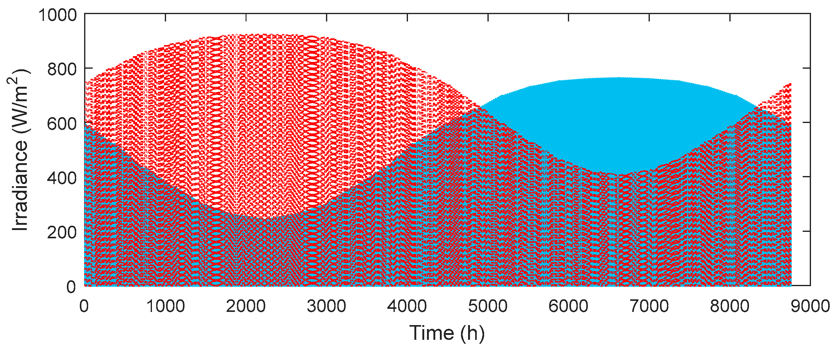
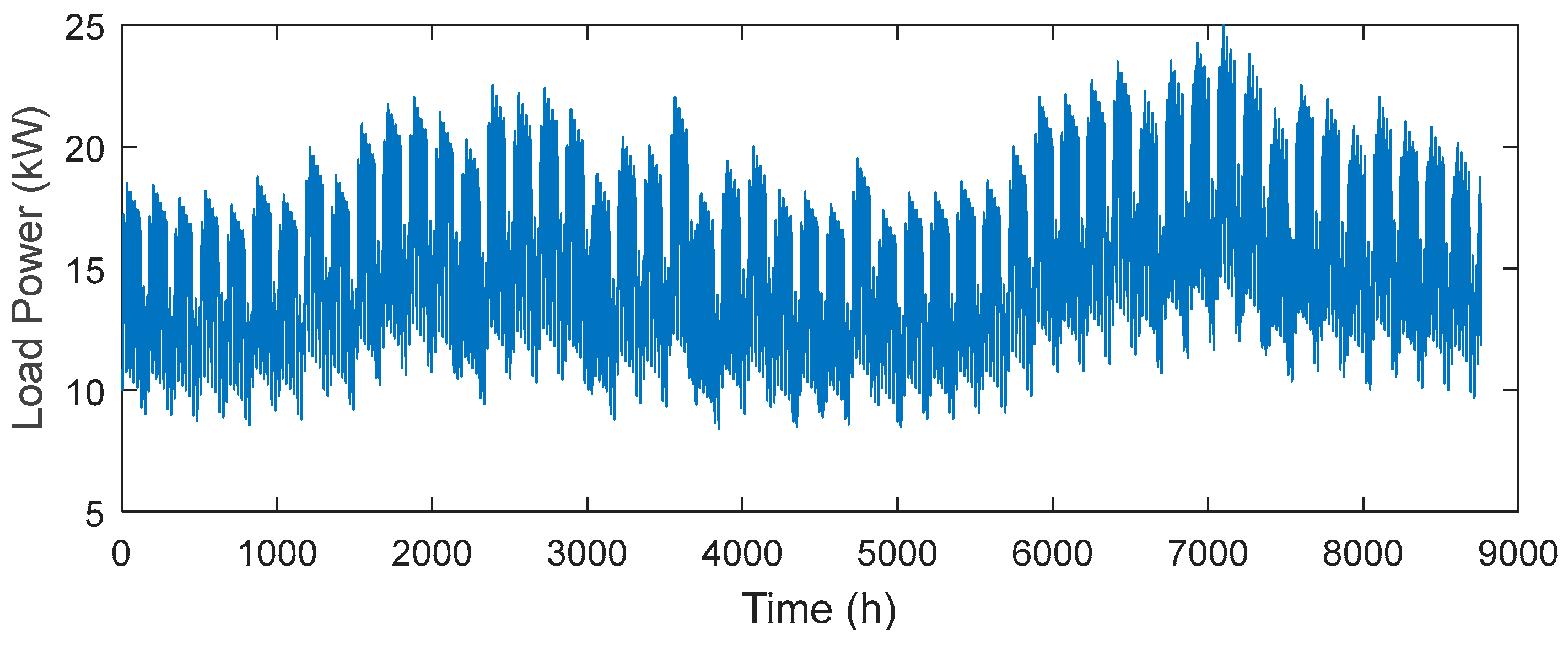
Initializing the data for an HRES, which include information on wind, irradiance, and load demand for a year, as well as numerical data pertaining to the size, cost, efficiency, and lifetime of the system’s components.

Step (2)

Commence the algorithm population, establish the maximum iteration, and determine the repetition. Additionally, the variables are generated randomly.

Step (3)

The COPL (Equation (16)) is computed for each algorithm’s member. This computation is performed on variables that have been randomly assigned while ensuring that they satisfy the POLS (Equation (20)).

Step (4)

Identification of the most optimal individual within the algorithm population is conducted by evaluating the individual’s COPL value, with preference given to those with lower COPL values, as well as considering their POLS performance, aiming for improved outcomes.

Step (5)

Proceed with the revision of the algorithm population.

Step (6)

The COPL meeting POLS is computed for members of the population identified in Step (5).

Step (7)

Identification of the optimal variable set characterized by the minimal COPL and superior POLS if the current COPL is less than the COPL calculated in Step (4), the current set is replaced with the latter.

Step (8)

Convergence metrics are evaluated. If these metrics meet the required criteria, we proceed to Step (10). However, if the convergence indices do not meet the required criteria, we must go to Step (5).

Step (9)

Set of variables that yield the ideal outcome is found.

Step (10)

Terminate the implementation of the algorithm.

6. Simulation Results and Discussion

6.1. System Data

In this section, the deterministic and stochastic sizing results for the hPV/HKT/FC, hPV/FC, and hHKT/FC configurations are presented to minimize the COPL while satisfying the POLS constraint. The system’s total yearly demand is 277,690 MW. The actual information on irradiance, wind speed, and annual variations in load are derived Ref. [27], where they are depicted in Figure 4, Figure 5 and Figure 6.

Table 2. The techno-economic data of the HRES components [27,30,31,48].

Device	${\partial }_{\mathit{C}\mathit{A}\mathit{P}}$ ($/Unit)	${\partial }_{\mathit{R}\mathit{E}\mathit{P}}$ ($/Unit)	${\partial }_{\mathit{M}\mathit{A}\mathit{I}\mathit{N}\mathit{O}\mathit{P}}$ ($/Unit-Year)	Rated Size	Efficiency	Life Span (Year)
PV	2000	500	33	1 kW	-	20
HKT	25,000	17,000	100	10 kW	-	20
EL	20,000	1400	100	3 kW	0.74	5
HST	1300	200	25	1 kg	0.95	20
FC	20,000	1400	100	3 kW	0.50	5
Inv	800	200	8	1 kW	0.90	15

provides techno-economic data of the HRES components derived from Refs. [27,30,31,48]. A study has been undertaken to evaluate the possibility and likelihood of constructing the proposed HRES in the Ardabil area. The objective of this research is to find the most reliable and economical system configuration for implementing an HRES based on PVs and HKTs, with hydrogen storage, taking into account stochastic sizing uncertainties. The proposed method is compared with conventional GBO (${\beta }_{min}=0.2, {\beta }_{max}=1.2, \mathrm{a}\mathrm{n}\mathrm{d} p_r=0.5$), particle swarm optimization (PSO) (c₁ and c₂ = 2, w_min = 0.1 and w_max = 0.9) [46], and artificial electric field algorithm (AEFA) (K₀ = 500) [47] to demonstrate its superiority. The general parameters of each algorithm are chosen based on their respective basis reference [43,46,47]. In addition, the population, maximum iteration, and repetition of each algorithm are considered to be 50, 200, and 30 using a combination of the authors’ knowledge. According to a 20-year project lifespan, the estimated interest and inflation rates are 9% and 3%, respectively. The utmost limit for HKTs, PVs, EL power, HST mass, FC power, and power injected by the inverter to the load are 1000, 1000, 1000, 1000, and 100, respectively, and the minimum limit for these variables is zero.

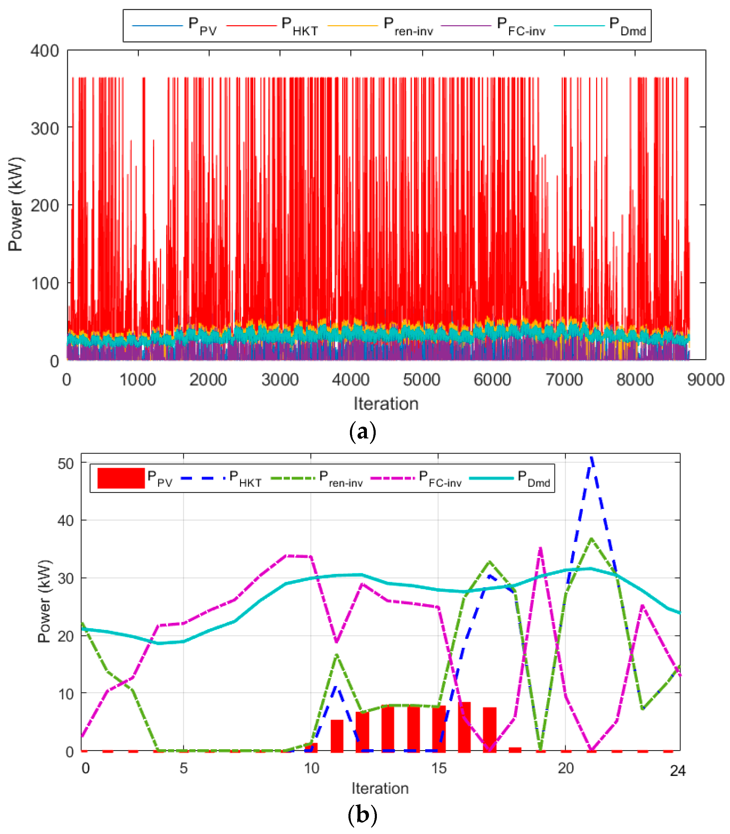
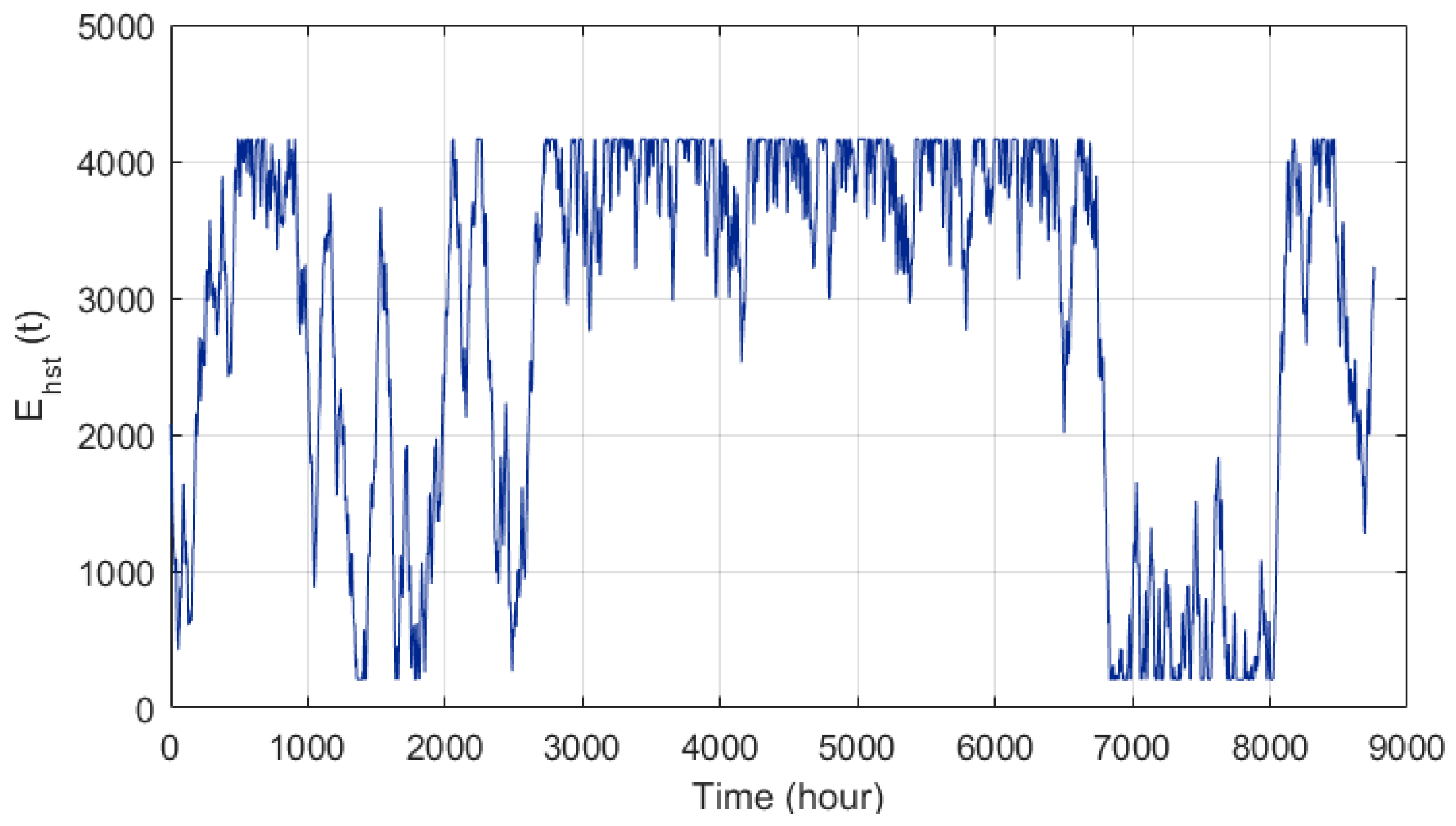
6.2. Results of Deterministic Sizing

The deterministic sizing results without uncertainty for various HRES configurations utilizing the IGBO method are presented. Figure 7 depicts the convergence curve obtained from the IGBO in solving the sizing of various hPV/HKT/FC, hPV/FC, and hHKT/FC configurations, which indicates that the hPV/HKT/FC and hHKT/FC configurations have obtained a lower COPL. It is also evident that the hPV/FC configuration has higher sizing costs than the other two configurations.

Table 3. The deterministic sizing results of the HRES using IGBO, case 1.

System Type/Item	${\mathrm{P}}_{\mathrm{H}\mathrm{K}\mathrm{T}} \left(\mathrm{k}\mathrm{W}\right)$	${\mathrm{P}}_{\mathrm{P}\mathrm{V}} \left(\mathrm{k}\mathrm{W}\right)$	${\mathsf{\theta }}_{\mathrm{P}\mathrm{V}}$	${\mathrm{P}}_{\mathrm{E}\mathrm{l}}$ $\left(\mathrm{k}\mathrm{W}\right)$	${\mathrm{M}}_{\mathrm{H}\mathrm{S}\mathrm{T}} \left(\mathrm{k}\mathrm{g}\right)$	${\mathrm{P}}_{\mathrm{F}\mathrm{C}} \left(\mathrm{k}\mathrm{W}\right)$	${\mathrm{P}}_{\mathrm{I}\mathrm{n}\mathrm{v}} \left(\mathrm{k}\mathrm{W}\right)$
hPV/HKT/FC	360.09	70.54	37.52	16.81	90.82	14.87	55.29
hPV/FC	--	1067.57	32.83	78.14	75.93	16.91	54.16
hHKT/FC	410.78	--	--	16.79	127.09	16.47	54.42

presents the numerical results of deterministic sizing without uncertainty for hPV/HKT/FC, hPV/FC, and hHKT/FC configurations employing the IGBO. Using the IGBO in case 1, the values of HKTs power, PVs power, EL power, HST mass, FC power, and injected power from the inverter to the load are as follows: 3600.9 kW, 70.54 kW, 16.81 kW, 90.82 kg, 14.87 kW, and 55.29 kW, respectively. In addition, according to the results in

Table 4. The reliability and cost results of deterministic sizing of the HRES using IGBO, case 1.

System Type/Item	$\mathrm{P}\mathrm{O}\mathrm{L}\mathrm{S}$	$\mathrm{B}\mathrm{e}\mathrm{s}\mathrm{t} \mathrm{C}\mathrm{O}\mathrm{P}\mathrm{L} \left(\mathrm{M}\mathrm{\$}\right)$	$\mathrm{M}\mathrm{e}\mathrm{a}\mathrm{n} \mathrm{C}\mathrm{O}\mathrm{P}\mathrm{L} \left(\mathrm{M}\mathrm{\$}\right)$	$\mathrm{W}\mathrm{o}\mathrm{r}\mathrm{s}\mathrm{t} \mathrm{C}\mathrm{O}\mathrm{P}\mathrm{L} \left(\mathrm{M}\mathrm{\$}\right)$	$\mathrm{s}\mathrm{t}\mathrm{d} \left(\mathrm{M}\mathrm{\$}\right)$
hPV/HKT/FC	0.0339	2.056	2.058	2.061	1174.69
hPV/FC	0.0401	4.952	4.961	4.981	5234.29
hHKT/FC	0.0370	2.131	2.132	2.137	700.05

, it is evident that the hPV/HKT/FC configuration is a reliable-economical energy configuration, as it achieved the lowest COPL and POLS, as well as the highest level of reliability when compared with other configurations. The resulting POLS values for hPV/HKT/FC, hPV/FC, and hHKT/FC configurations are 0.0339, 0.0401, and 0.0370, and the COPL values for these configurations are 2.056 M$, 2.131 M$, and 4.952 M$, respectively. By overlapping PV and HKT energy sources with hydrogen reserve power, the results cleared that the hPV/HKT/FC configuration has superior performance. The results demonstrated that the total cost of sizing the hPV/FC configuration with only PV production resources and hydrogen storage is significantly higher than the other two configurations and is not cost-effective in comparison to them. It is also evident from the results that the hHKT/FC configuration, which follows hPV/HKT/FC in terms of efficacy, has the highest cost and the lowest level of reliability.

In Figure 8, the cost contribution for components in each of the different configurations is presented. In the hPV/HKT/FC configuration the HKT resources (46%), in the hPV/FC configuration the PV resources (51%) and in the hHKT/FC configuration the HKT resources (51%) account for the highest percentage of the total cost (COPL); moreover, the inverter is the piece of equipment that has the lowest cost share among the equipment of any configuration.

Figure 9 illustrates the yearly and daily contribution provided by each system component to the hPV/HKT/FC sizing solution. On the basis of Figure 9 and (b) and the overlap of HKT and PV sources in addition to hydrogen storage and fuel cell production power, the required load energy has been supplied with a reliability of 96.61% ($(1-\left(0.0339/1\right))\times 100$). In addition, Figure 10 illustrates the HST energy variations, which demonstrates how the hydrogen tank with hydrogen charging and discharging and intelligent management of hydrogen reserve power (particularly hours 1000 to 2500 and hours 7000 to 8000) generates electrical scheduling and continual supply of the load at an appropriate level of reliability.

In Figure 11, the yearly variations of POLS for the hPV/HKT/FC configuration are plotted, and it is evident that the demand is entirely provided in the majority of hours, with the exception of a few hours in which the load is greater than other hours and a portion of the load cannot be met naturally. Consequently, 3.39% of the total load has not been supplied considering $POL{S}_{\max }=5\%$.

In following, the IGBO’s ability to solve the deterministic sizing problem for the optimal hPV/HKT/FC configuration is contrasted to that of other algorithms, such as the traditional GBO, PSO, and AEFA. Figure 12 depicts the convergence curve resulting from the optimization process by various algorithms, and as can be seen, the method outlined in this study accomplished a lower cost objective function value than other methods. It has been demonstrated that utilizing the dynamic lens-imaging learning technique to enhance the performance of the traditional GBO has enhanced the algorithm’s exploration, decreased its convergence tolerance, and increased its convergence rate.

In

Table 5. Sizing results of the hPV/HKT/FC system via different algorithms.

System Type/Item	${\mathrm{P}}_{\mathrm{H}\mathrm{K}\mathrm{T}}\left(\mathrm{k}\mathrm{W}\right)$	${\mathrm{P}}_{\mathrm{P}\mathrm{V}}\left(\mathrm{k}\mathrm{W}\right)$	${\mathsf{\theta }}_{\mathrm{P}\mathrm{V}}$	${\mathrm{P}}_{\mathrm{E}\mathrm{l}}$ $\left(\mathrm{k}\mathrm{W}\right)$	${\mathrm{M}}_{\mathrm{H}\mathrm{S}\mathrm{T}}\left(\mathrm{k}\mathrm{g}\right)$	${\mathrm{P}}_{\mathrm{F}\mathrm{C}}\left(\mathrm{k}\mathrm{W}\right)$	${\mathrm{P}}_{\mathrm{I}\mathrm{n}\mathrm{v}}\left(\mathrm{k}\mathrm{W}\right)$
IGBO	360.09	70.54	37.52	16.81	90.82	14.87	55.29
GBO	420.85	32.54	33.95	16.20	118.47	16.75	54.80
PSO	410.88	24.66	30.67	16.74	123.70	15.86	55.10
AEFA	350.49	85.68	38.99	16.27	143.56	14.88	55.04

and

Table 6. Cost and reliability results of the hPV/HKT/FC system sizing via different algorithms.

System Type/Item	$\mathrm{P}\mathrm{O}\mathrm{L}\mathrm{S}$	$\mathrm{B}\mathrm{e}\mathrm{s}\mathrm{t} \mathrm{C}\mathrm{O}\mathrm{P}\mathrm{L} \left(\mathrm{M}\mathrm{\$}\right)$	$\mathrm{M}\mathrm{e}\mathrm{a}\mathrm{n} \mathrm{C}\mathrm{O}\mathrm{P}\mathrm{L} \left(\mathrm{M}\mathrm{\$}\right)$	$\mathrm{W}\mathrm{o}\mathrm{r}\mathrm{s}\mathrm{t} \mathrm{C}\mathrm{O}\mathrm{P}\mathrm{L} \left(\mathrm{M}\mathrm{\$}\right)$	$\mathrm{s}\mathrm{t}\mathrm{d} \left(\mathrm{M}\mathrm{\$}\right)$
IGBO	0.0339	2.056	2.058	2.061	374.69
GBO	0.0375	2.376	2.381	2.389	1265.55
PSO	0.0355	2.132	2.133	2.135	417.65
AEFA	0.0394	2.152	2.157	2.161	1064.49

, the deterministic sizing results, including the optimal variable set, as well as the cost and reliability results gained using various algorithms are displayed. It can be observed that the proposed IGBO takes the system with the greatest amount of reliability (lowest POLS) and the lowest COPL when compared with other methods. Using IGBO, GBO, PSO, and AEFA, the PLOS value is 0.0339, 0.0394, 0.0355, and 0.0375, respectively, and the best COPL value is 2.056 M$, 2.152 M$, 2.132 M$, and 2.138 M$, respectively, demonstrating that IGBO is preferable to other algorithms for sizing hPV/HKT/FC.

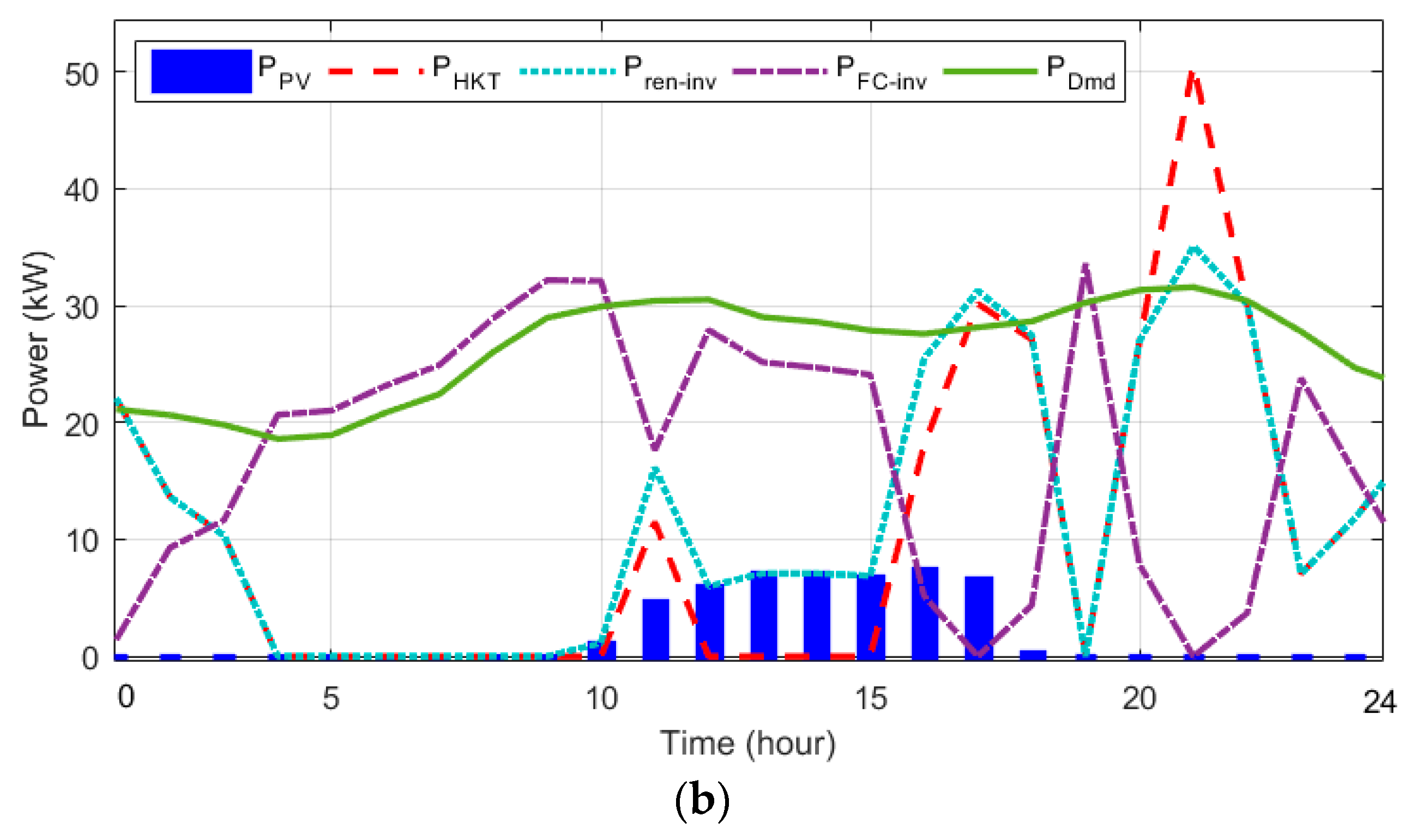
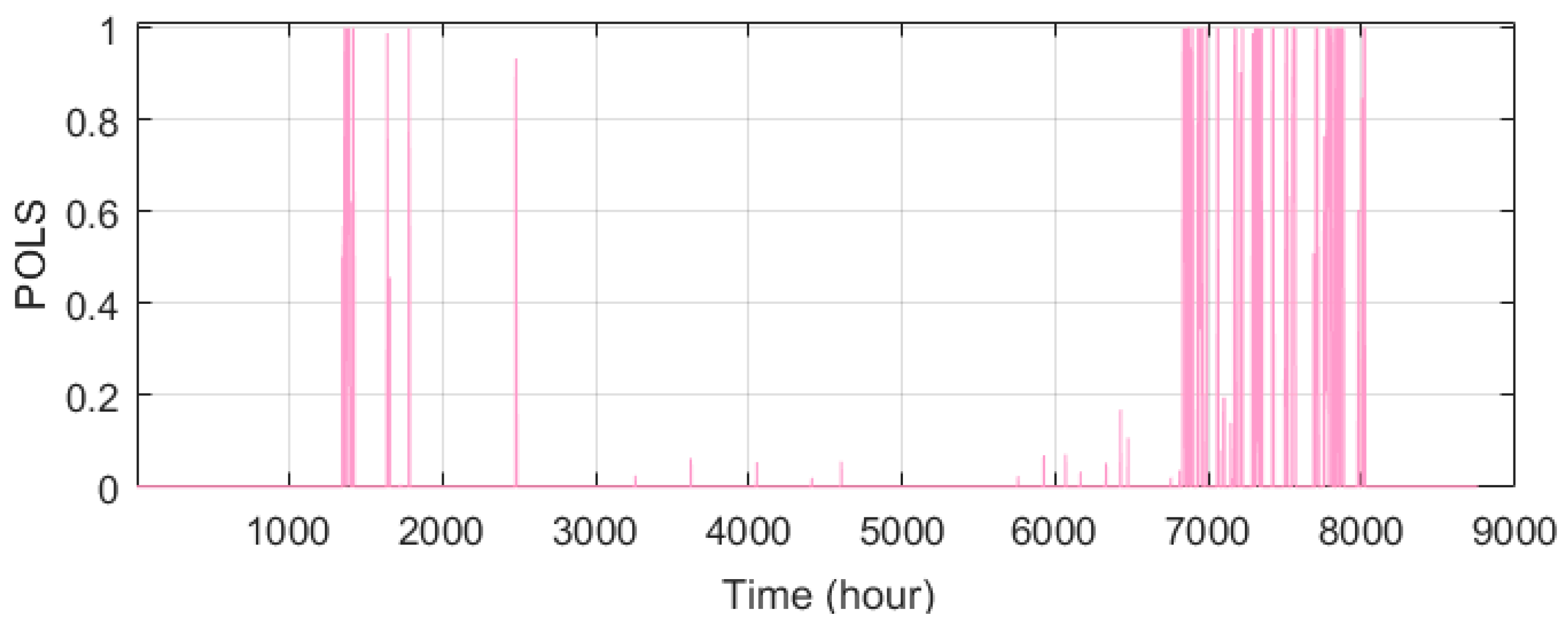
6.3. Results of Stochastic Sizing

The results of stochastic sizing of different HRES combinations based on the 2m+1 PEM approach incorporating RESs generation and demand uncertainties for the hPV/HKT/FC, hPV/FC, and hHKT/FC configurations using the IGBO method are given in

Table 7. The deterministic sizing results of the HRES using IGBO, case 2.

System Type/Item	${\mathrm{P}}_{\mathrm{H}\mathrm{K}\mathrm{T}}\left(\mathrm{k}\mathrm{W}\right)$	${\mathrm{P}}_{\mathrm{P}\mathrm{V}}\left(\mathrm{k}\mathrm{W}\right)$	${\mathsf{\theta }}_{\mathrm{P}\mathrm{V}}$	${\mathrm{P}}_{\mathrm{E}\mathrm{l}}$ $\left(\mathrm{k}\mathrm{W}\right)$	${\mathrm{M}}_{\mathrm{H}\mathrm{S}\mathrm{T}}\left(\mathrm{k}\mathrm{g}\right)$	${\mathrm{P}}_{\mathrm{F}\mathrm{C}}\left(\mathrm{k}\mathrm{W}\right)$	${\mathrm{P}}_{\mathrm{I}\mathrm{n}\mathrm{v}}\left(\mathrm{k}\mathrm{W}\right)$
hPV/HKT/FC	380.32	82.25	39.46	18.25	104.79	15.59	55.76
hPV/FC	--	1179.09	36.11	82.09	79.74	17.38	54.69
hHKT/FC	460.31	--	--	17.57	135.15	17.12	54.86

. According to Table 7, the values of HKTs power, PVs power, EL power, HST mass, FC power, and sent power by the inverter to the load are obtained 38.32 kW, 82.25 kW, 18.25 kW, 104.79 kg, 15.59 kW, and 55.76 kW, respectively using the IGBO in case 2. According to the results in

Table 8. The reliability and cost results of deterministic sizing of the HRES using IGBO, case 2.

System Type/Item	$\mathrm{P}\mathrm{O}\mathrm{L}\mathrm{S}$	$\mathrm{B}\mathrm{e}\mathrm{s}\mathrm{t} \mathrm{C}\mathrm{O}\mathrm{P}\mathrm{L} \left(\mathrm{M}\mathrm{\$}\right)$	$\mathrm{M}\mathrm{e}\mathrm{a}\mathrm{n} \mathrm{C}\mathrm{O}\mathrm{P}\mathrm{L} \left(\mathrm{M}\mathrm{\$}\right)$	$\mathrm{W}\mathrm{o}\mathrm{r}\mathrm{s}\mathrm{t} \mathrm{C}\mathrm{O}\mathrm{P}\mathrm{L} \left(\mathrm{M}\mathrm{\$}\right)$	$\mathrm{s}\mathrm{t}\mathrm{d} \left(\mathrm{M}\mathrm{\$}\right)$
hPV/HKT/FC	0.0322	2.213	2.214	2.218	965.44
hPV/FC	0.0383	5.327	5.332	5.349	3203.55
hHKT/FC	0.0353	2.294	2296	2298	777.06

, it is clear that hPV/HKT/FC is the optimal configuration because it obtained the lowest COPL and the lowest POLS compared with other configurations. The POLS for hPV/HKT/FC, hPV/FC, and hHKT/FC configurations are obtained 0.0322, 0.0383, and 0.0353, respectively, and the COPL for hPV/HKT/FC, hPV/FC, and hHKT/FC configurations are calculated 2.213 M$, 5.327 M$, and 2.294 M$, respectively. Therefore, the results demonstrated the better performance of the hPV/HKT/FC configuration by overlapping PV and HKT resources with hydrogen storage energy. The results demonstrated that the total cost of sizing the hPV/FC configuration using only PV production resources with hydrogen storage is much higher than the other two combinations and, like case 1, it is not economical compared to them. Additionally, similarly to the deterministic case, it is clear from the stochastic sizing results that hHKT/FC configuration after hPV/HKT/FC has the best performance but with a higher cost and lower reliability level.

In Figure 13, annual and daily contributions of each system components for hPV/HKT/FC stochastic sizing are depicted. Based on Figure 13 and (b), with the overlap of HKT and PV resources, as well as hydrogen storage and FC production power, the required load energy has been supplied with a reliability of 96.78% ($(1-\left(0.0322/1\right))\times 100$). Additionally, the HST energy curve is presented in Figure 14, which shows that the hydrogen tank with hydrogen charging and discharging, and intelligent management of hydrogen reserve power has created electrical scheduling and a continuous supply of load with a suitable level of reliability.

In Figure 15, the annual variation of POLS for the hPV/HKT/FC configuration in stochastic sizing based on the 2m+1 PEM approach is presented, which shows that most of the load hours are fully supplied, with the exception of some hours in which the load is greater than other hours and part of the load is not provided. In other words, 3.22% of the total load considering $POL{S}_{\max }=5\%$ is not supplied.

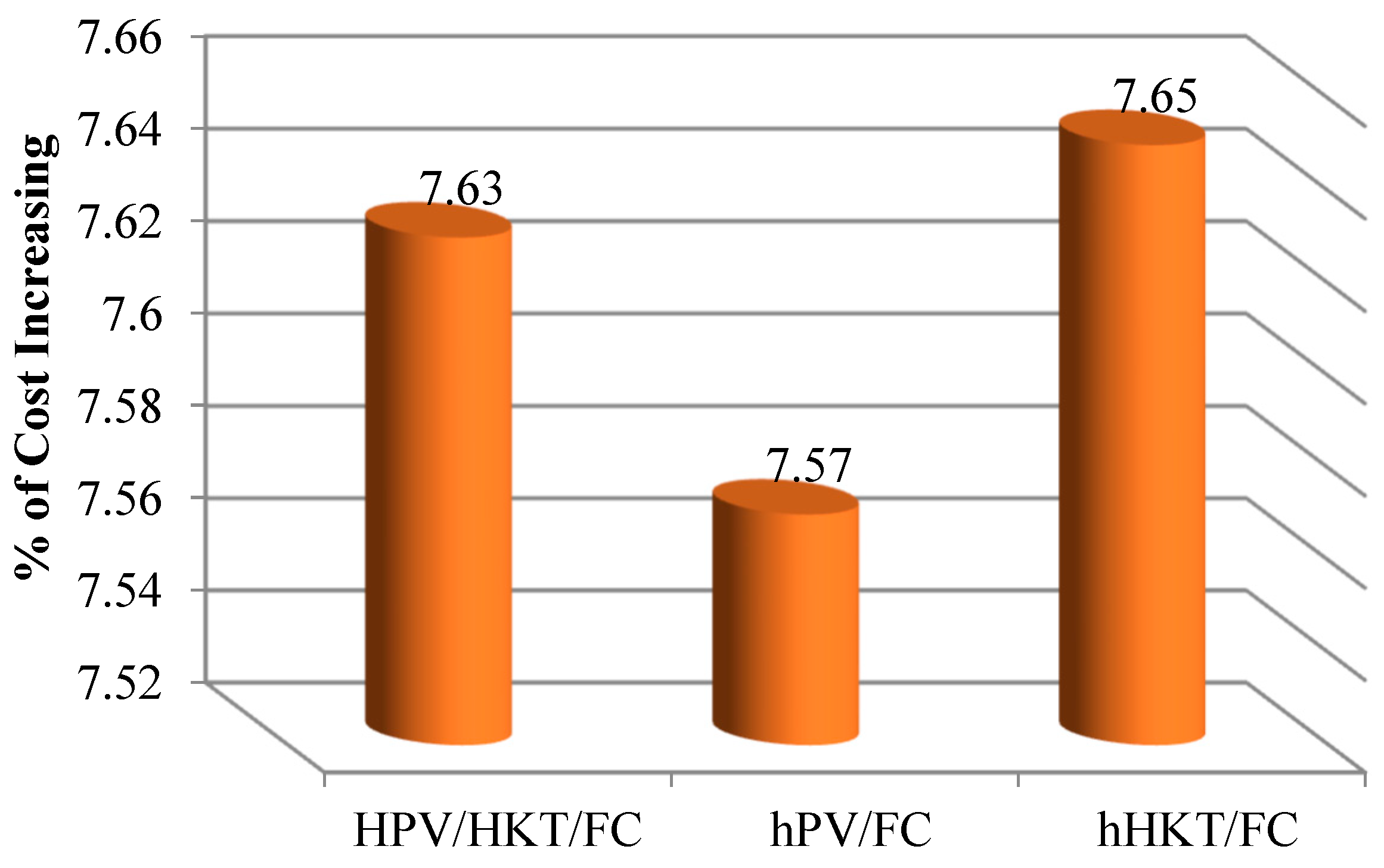
6.4. Deterministic and Stochastic Results Comparison

Examining the results revealed that in order to accomplish the desired reliability, at least as in deterministic sizing, it is required to increase the level of power production and storage (see Figure 16) in different configurations of the HRES in order to use the proposed method under stochastic sizing conditions with the uncertainty of energy production sources and system load. In this manner, stochastic conditions result in a greater degree of production and storage level determination than deterministic measurement. Consequently, the results demonstrated that the storage level obtained from deterministic sizing does not guarantee the load requirement under uncertain conditions; thus, the proposed program raised the renewable production level, particularly the hydrogen storage value, to more precisely support the load requirements.

As shown in

Table 9. The results comparison of deterministic and stochastic sizing for HRES different configuration.

System/Item	Approach	${\mathrm{P}}_{\mathrm{H}\mathrm{K}\mathrm{T}}\left(\mathrm{k}\mathrm{W}\right)$	${\mathrm{P}}_{\mathrm{P}\mathrm{V}}\left(\mathrm{k}\mathrm{W}\right)$	${\mathsf{\theta }}_{\mathrm{P}\mathrm{V}}$	${\mathrm{P}}_{\mathrm{E}\mathrm{l}}$ $\left(\mathrm{k}\mathrm{W}\right)$	${\mathrm{M}}_{\mathrm{H}\mathrm{S}\mathrm{T}}\left(\mathrm{k}\mathrm{g}\right)$	${\mathrm{P}}_{\mathrm{F}\mathrm{C}}\left(\mathrm{k}\mathrm{W}\right)$	${\mathrm{P}}_{\mathrm{I}\mathrm{n}\mathrm{v}}\left(\mathrm{k}\mathrm{W}\right)$	$\mathrm{P}\mathrm{O}\mathrm{L}\mathrm{S}$	$\mathrm{C}\mathrm{O}\mathrm{P}\mathrm{L}$
hPV/HKT/FC	Deterministic	36.09	70.54	37.52	16.81	90.82	14.87	55.29	0.0339	2.056
	Stochastic	38.32	82.25	39.46	18.25	104.79	15.59	55.76	0.0322	2.213
hPV/FC	Deterministic	--	1067.57	32.83	78.14	75.93	16.91	54.16	0.0401	4.952
	Stochastic	--	1179.09	36.11	82.09	79.74	17.38	54.69	0.0383	5.327
hHKT/FC	Deterministic	41.78	--	--	16.79	127.09	16.47	54.42	0.0370	2.131
	Stochastic	46.31	--	--	17.57	135.15	17.12	54.86	0.0353	2.294

COPL: M$.

and Figure 17, the value of COPL for hPV/HKT/FC, hPV/FC, and hHKT/FC configurations increased by 7.63%, 7.57%, and 7.65%, respectively, in stochastic sizing compared with deterministic sizing. In addition, according to Table 9 and Figure 18, the value of POLS for hPV/HKT/FC, hPV/FC, and hHKT/FC configurations in stochastic sizing has declined by 5.01%, 4.48%, and 4.59%, respectively, when compared to deterministic sizing. Consequently, deterministic sizing cannot provide energy system operators with accurate knowledge of design costs and levels of reliability, whereas stochastic sizing, which accounts for uncertainties, can result in correct scheduling and optimal load demand support with accurate knowledge of cost and reliability values.

According to Figure 19, the lower cost for each equipment is obtained for the optimal hPV/HKT/FC combination. Figure 19 shows the component costs of different system configurations for deterministic and stochastic sizing problems. HKTs have the largest cost contribution in the hPV/HKT/FC and hHKT/FC configurations when using deterministic and stochastic measurement techniques. In the hPV/FC configuration, PVs have the largest cost share. The inverter has the lowest cost contribution in all configurations for both measurement methods. Therefore, HKTs energy sources have the largest share of cost in the sizing of hybrid energy systems. Therefore, in the optimal combination, their participation with PV sources has reduced sizing costs.

6.5. Comparison with Previous Studies

In this section,

Table 10. Results comparison with previous studies.

Ref.	HRES Type	Stochastic Sizing	COE ($/kWh)
Homer [50]	PV/Wind/FC	✕	0.83
FPA [27]	PV/WT/FC	✕	0.52
WOA [42]	PV/HKT/FC	✕	0.4546
This paper	PV/HKT/FC	✓	0.3984

is used to compare the results derived from the optimal configuration in terms of cost of energy (COE) to supply each kilowatt-hour of load demand with those of previous studies. It should be noted, however, that meteorological data is one of the most important factors in hybrid energy system measurement. Therefore, in this comparison, the higher or lower COE does not indicate the superiority of the method; rather, it reveals that the COE of each region differs from another region due to weather conditions and meteorological data differences. According to the 277,690 kWh load demand, the COE for the stochastic method proposed in this study is 2213 M$ and the 20-year project life span is 0.3984 $/kWh. The results demonstrated that the integration of the stochastic methodology proposed in this study with the meteorological data of the Ardabil region has a lower COE than other studies, particularly Ref. [42], which has the same HRES but a different methodology.

6.6. Discussion

In order to reduce the COPL while still meeting the POLS requirement, the deterministic and stochastic sizing of the hPV/HKT/FC, hPV/FC, and hHKT/FC configurations are provided in this work. For various HRES configurations using the IGBO approach, the deterministic sizing results without uncertainty are first retrieved.

The hPV/FC design has greater sizing costs than the other two configurations, according to the deterministic results, which also demonstrated that the hPV/HKT/FC and hHKT/FC configurations have achieved lower COPLs. The hPV/HKT/FC configuration achieved the lowest COPL and POLS, as well as the best level of reliability when compared with other configurations, and the hHKT/FC configuration has the highest cost and the lowest degree of reliability, proving that it is a reliable economical energy configuration. The findings showed that the HKT resources account for the highest percentage of the total cost (COPL) in the hPV/HKT/FC configuration (46%) followed by the PV resources (51%) and the HKT resources (51%) in the hPV/FC configuration. Additionally, the IGBO’s superiority is contrasted with that of the traditional GBO, PSO, and AEFA algorithms. The results showed that the dynamic lens-imaging learning technique improved the exploration, decreased the convergence tolerance, and increased the convergence rate of the traditional GBO, making the IGBO superior to other algorithms for sizing the hPV/HKT/FC configuration. The stochastic results show that the required load energy has been delivered with a reliability of 96.61% based on the hPV/HKT/FC.

Then, utilizing the IGBO, stochastic sizing of various HRES combinations is accomplished based on the 2m+1 PEM approach, taking into account the uncertainties in RESs generation and demand for the hPV/HKT/FC, hPV/FC, and hHKT/FC configurations. The hPV/HKT/FC arrangement performs better than other configurations due to the mixture of PV and HKT resources with hydrogen storage energy. According to the results, this design is best since it acquired the lowest COPL and lowest POLS relative to other configurations. The stochastic sizing findings show that similar to the deterministic scenario, the hHKT/FC configuration after hPV/HKT/FC has the highest performance but at a greater cost and poorer reliability level. The stochastic results show that the required load energy has been delivered with a reliability of 96.78% based on the hPV/HKT/FC.

The outcomes of stochastic and deterministic sizing are then contrasted. In comparison to deterministic sizing, stochastic conditions lead to higher levels of production and storage. The proposed program increased the renewable production level, notably the hydrogen storage value, to more precisely support the load requirements as it was determined that the storage level derived by deterministic sizing does not ensure the load demand under unknown situations. Furthermore, when uncertainty based on stochastic sizing as opposed to deterministic sizing is taken into account, the COPL for the hPV/HKT/FC, hPV/FC, and hHKT/FC configurations increased by 7.63%, 7.57%, and 7.65%, respectively, and the POLS had decreased by 5.01%, 4.48%, and 4.59%, respectively.

7. Conclusions

In this paper, stochastic sizing of different configurations of an off-grid HRES incorporating hydrogen energy storage was implemented using 2m+1 PEM and IGBO to minimize the COPL satisfying the POLS. The 2m+1 PEM addresses the limitations associated with the approximations by utilizing the initial statistical moments applied to model the RESs generation and demand uncertainties. The effectiveness of the proposed stochastic sizing was compared with the deterministic sizing without uncertainty. The outcomes of the study are presented as below:

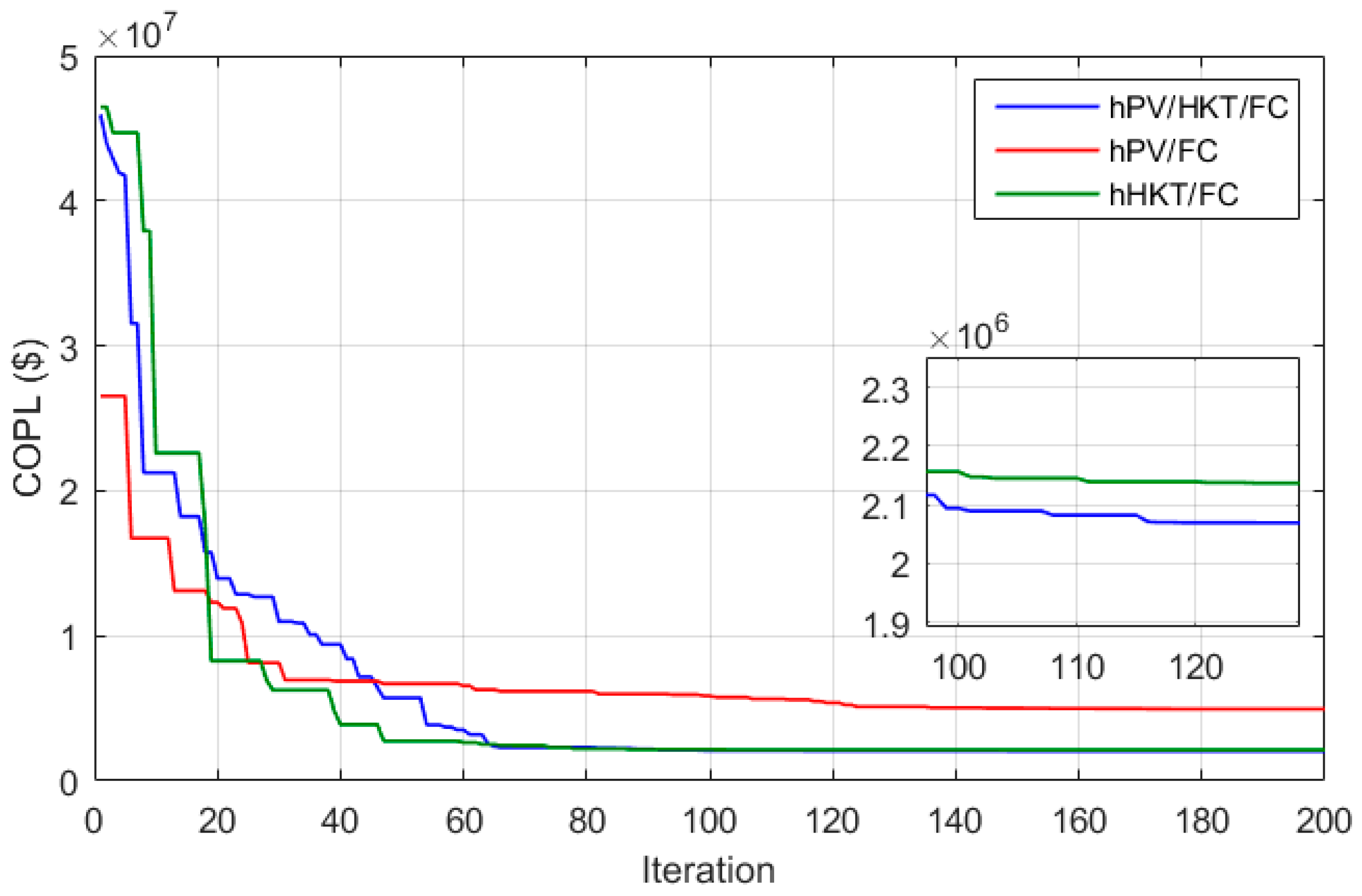
• The deterministic results cleared that the hPV/HKT/FC configuration was the optimal with lowest COPL and POLS (highest reliability level) and the hPV/FC configuration obtained higher COPL and POLS. COPL and POLS achieved 0.0339 and 2.056 M$, for the hPV/HKT/FC configuration and for hPV/FC configuration they obtained 0.0401 and 2.131 M$, respectively.
• The findings proved the superior sizing capability of the IGBO compared with conventional GBO, PSO, and GWO methods with the lowest COPL and POLS. The results of the comparison of the algorithms confirmed the capability of the dynamic lens-imaging learning technique to improve the conventional GBO performance in achieving the best solution with less convergence tolerance.
• The stochastic sizing results showed that the hPV/HKT/FC configuration was obtained as the optimal configuration for the lowest obtained COPL and POLS compared with other configurations; moreover, the hPV/FC was introduced as an expensive configuration. The COPL and POLS for optimal configuration were obtained at 0.0322 and 2.213 M$ and were also achieved at 0.0383 and 5.327 M$, respectively, for expensive configuration.
• Therefore, the results demonstrated that the storage level obtained in deterministic sizing does not guarantee the load requirement in the conditions of uncertainty that the proposed stochastic sizing increased the renewable production level and also hydrogen storage level to more accurately support the load needs. In other words, stochastic sizing, taking into account uncertainties, can lead to correct scheduling and optimal load demand support with the correct knowledge of values of cost and reliability.
• The robust sizing and energy management of the hPV/HKT/FC energy system with multi-energy storage using the information gap decision theory is suggested for future work. In other words, in this proposed plan, the effect of using the robust method compared to the stochastic method will be investigated in terms of uncertainty on the sizing problem considering battery and hydrogen-based energy storage.
• Additionally, the stochastic sizing of the hPV/HKT energy system integrated with different technologies of battery energy storage is suggested for future work. In this project, the effect of various battery technologies, including lithium-ion and Vanadium redox batteries, on solving the sizing problem under conditions of uncertainty will be evaluated.

References

1. Sarker, A.K.; Azad, A.K.; Rasul, M.G.; Doppalapudi, A.T. Prospect of Green Hydrogen Generation from Hybrid Renewable Energy Sources: A Review. Energies 2023, 16, 1556. [Google Scholar] [CrossRef]
2. Huang, S.; Huang, M.; Lyu, Y. Seismic performance analysis of a wind turbine with a monopile foundation affected by sea ice based on a simple numerical method. Eng. Appl. Comput. Fluid Mech. 2021, 15, 1113–1133. [Google Scholar] [CrossRef]
3. Zhang, Z.; Altalbawy, F.M.; Al-Bahrani, M.; Riadi, Y. Regret-based multi-objective optimization of carbon capture facility in CHP-based microgrid with carbon dioxide cycling. J. Clean. Prod. 2023, 384, 135632. [Google Scholar] [CrossRef]
4. Mahzouni-Sani, M.; Hamidi, A.; Nazarpour, D.; Golshannavaz, S. Multi-objective linearised optimal reactive power dispatch of wind-integrated transmission networks. IET Gener. Transm. Distrib. 2019, 13, 2686–2696. [Google Scholar] [CrossRef]
5. Baghban-Novin, S.; Mahzouni-Sani, M.; Hamidi, A.; Golshannavaz, S.; Nazarpour, D.; Siano, P. Investigating the impacts of feeder reforming and distributed generation on reactive power demand of distribution networks. Sustain. Energy Grids Netw. 2020, 22, 100350. [Google Scholar] [CrossRef]
6. Fathi, R.; Tousi, B.; Galvani, S. A new approach for optimal allocation of photovoltaic and wind clean energy resources in distribution networks with reconfiguration considering uncertainty based on info-gap decision theory with risk aversion strategy. J. Clean. Prod. 2021, 295, 125984. [Google Scholar] [CrossRef]
7. Rostami, A.; Mohammadi, M.; Karimipour, H. Reliability assessment of cyber-physical power systems considering the impact of predicted cyber vulnerabilities. Int. J. Electr. Power Energy Syst. 2023, 147, 108892. [Google Scholar] [CrossRef]
8. Liu, Z.; Tang, P.; Hou, K.; Zhu, L.; Zhao, J.; Jia, H.; Pei, W. A Lagrange-multiplier-based Reliability Assessment for Power Systems Considering Topology and Injection Uncertainties. IEEE Trans. Power Syst. 2023, 1–11. [Google Scholar] [CrossRef]
9. Crooks, J.M.; Hewlin, R.L., Jr.; Williams, W.B. Computational Design Analysis of a Hydrokinetic Hori-zontal Parallel Stream Direct Drive Counter-Rotating Darrieus Turbine System: A Phase One Design Analysis Study. Energies 2022, 15, 8942. [Google Scholar] [CrossRef]
10. Kirke, B. Hydrokinetic turbines for moderate sized rivers. Energy Sustain. Dev. 2020, 58, 182–195. [Google Scholar] [CrossRef] [PubMed]
11. Saini, G.; Saini, R.P. Clearance and blockage effects on hydrodynamic performance of hybrid hydrokinetic turbine. Sustain. Energy Technol. Assess. 2023, 57, 103210. [Google Scholar] [CrossRef]
12. Li, M.; Yang, M.; Yu, Y.; Lee, W.J. A wind speed correction method based on modified hidden Markov model for enhancing wind power forecast. IEEE Trans. Ind. Appl. 2021, 58, 656–666. [Google Scholar] [CrossRef]
13. Chen, H.; Wu, H.; Kan, T.; Zhang, J.; Li, H. Low-carbon economic dispatch of integrated energy system containing electric hydrogen production based on VMD-GRU short-term wind power prediction. Int. J. Electr. Power Energy Syst. 2023, 154, 109420. [Google Scholar] [CrossRef]
14. Zhang, L.; Sun, C.; Cai, G.; Koh, L.H. Charging and discharging optimization strategy for electric vehicles considering elasticity demand response. eTransportation 2023, 18, 100262. [Google Scholar] [CrossRef]
15. Alanazi, M.; Alanazi, A.; Almadhor, A.; Rauf, H.T. An Improved Fick’s Law Algorithm Based on Dynamic Lens-Imaging Learning Strategy for Planning a Hybrid Wind/Battery Energy System in Distribution Network. Mathematics 2023, 11, 1270. [Google Scholar] [CrossRef]
16. Shezan, S.A.; Kamwa, I.; Ishraque, M.F.; Muyeen, S.M.; Hasan, K.N.; Saidur, R.; Rizvi, S.M.; Shafiullah, M.; Al-Sulaiman, F.A. Evaluation of different optimization techniques and control strategies of hybrid microgrid: A review. Energies 2023, 16, 1792. [Google Scholar] [CrossRef]
17. Aschidamini, G.L.; da Cruz, G.A.; Resener, M.; Ramos, M.J.; Pereira, L.A.; Ferraz, B.P.; Haffner, S.; Pardalos, P.M. Expansion Planning of Power Distribution Systems Considering Reliability: A Comprehensive Review. Energies 2022, 15, 2275. [Google Scholar] [CrossRef]
18. Kiehbadroudinezhad, M.; Merabet, A.; Hosseinzadeh-Bandbafha, H. Review of latest advances and prospects of energy storage systems: Considering economic, reliability, sizing, and environmental impacts approach. Clean Technol. 2022, 4, 477–501. [Google Scholar] [CrossRef]
19. Cai, T.; Dong, M.; Chen, K.; Gong, T. Methods of participating power spot market bidding and settlement for renewable energy systems. Energy Rep. 2022, 8, 7764–7772. [Google Scholar] [CrossRef]
20. Liu, Z.; Li, H.; Hou, K.; Xu, X.; Jia, H.; Zhu, L.; Mu, Y. Risk assessment and alleviation of regional integrated energy system considering cross-system failures. Appl. Energy 2023, 350, 121714. [Google Scholar] [CrossRef]
21. Jiang, J.; Zhang, L.; Wen, X.; Valipour, E.; Nojavan, S. Risk-based performance of power-to-gas storage technology integrated with energy hub system regarding downside risk constrained approach. Int. J. Hydrogen Energy 2022, 47, 39429–39442. [Google Scholar] [CrossRef]
22. Menesy, A.S.; Sultan, H.M.; Habiballah, I.O.; Masrur, H.; Khan, K.R.; Khalid, M. Optimal Configuration of a Hybrid Photovoltaic/Wind Turbine/Biomass/Hydro-Pumped Storage-Based Energy System Using a Heap-Based Optimization Algorithm. Energies 2023, 16, 3648. [Google Scholar] [CrossRef]
23. Jin, H.; Yang, X. Bilevel Optimal Sizing and Operation Method of Fuel Cell/Battery Hybrid All-Electric Shipboard Microgrid. Mathematics 2023, 11, 2728. [Google Scholar] [CrossRef]
24. Ghoniem, R.M.; Alahmer, A.; Rezk, H.; As’ad, S. Optimal Design and Sizing of Hybrid Photovoltaic/Fuel Cell Electrical Power System. Sustainability 2023, 15, 12026. [Google Scholar] [CrossRef]
25. Mohammed, A. An Optimization-Based Model for A Hybrid Photovoltaic-Hydrogen Storage System for Agricultural Operations in Saudi Arabia. Processes 2023, 11, 1371. [Google Scholar] [CrossRef]
26. Sanajaoba, S. Optimal sizing of off-grid hybrid energy system based on minimum cost of energy and reliability criteria using firefly algorithm. Sol. Energy 2019, 188, 655–666. [Google Scholar] [CrossRef]
27. Pires, A.L.G.; Junior, P.R.; Rocha, L.C.S.; Peruchi, R.S.; Janda, K.; de Carvalho Miranda, R. Environmental and financial multi-objective optimization: Hybrid wind-photovoltaic generation with battery energy storage systems. J. Energy Storage 2023, 66, 107425. [Google Scholar] [CrossRef]
28. Naderipour, A.; Nowdeh, S.A.; Saftjani, P.B.; Abdul-Malek, Z.; Mustafa, M.W.B.; Kamyab, H.; Davoudkhani, I.F. Deterministic and probabilistic multi-objective placement and sizing of wind renewable energy sources using improved spotted hyena optimizer. J. Clean. Prod. 2021, 286, 124941. [Google Scholar] [CrossRef]
29. Mahesh, A.; Sushnigdha, G. Optimal sizing of photovoltaic/wind/battery hybrid renewable energy system including electric vehicles using improved search space reduction algorithm. J. Energy Storage 2022, 56, 105866. [Google Scholar] [CrossRef]
30. Zhang, W.; Zheng, Z.; Liu, H. Droop control method to achieve maximum power output of photovoltaic for parallel inverter system. CSEE J. Power Energy Syst. 2021, 8, 1636–1645. [Google Scholar]
31. Jahannoosh, M.; Nowdeh, S.A. Optimal designing and management of a stand-alone hybrid energy system using meta-heuristic improved sine-cosine algorithm for Recreational Center, case study for Iran country. Appl. Soft Comput. 2020, 96, 106611. [Google Scholar] [CrossRef]
32. Niveditha, N.; Singaravel, M.R. Optimal sizing of hybrid PV–Wind–Battery storage system for Net Zero Energy Buildings to reduce grid burden. Appl. Energy 2022, 324, 119713. [Google Scholar] [CrossRef]
33. Maleki, A.; Nazari, M.A.; Pourfayaz, F. Harmony search optimization for optimum sizing of hybrid solar schemes based on battery storage unit. Energy Rep. 2020, 6, 102–111. [Google Scholar] [CrossRef]
34. Ridha, H.M.; Gomes, C.; Hizam, H.; Mirjalili, S. Multiple scenarios multi-objective salp swarm optimization for sizing of standalone photovoltaic system. Renew. Energy 2020, 153, 1330–1345. [Google Scholar] [CrossRef]
35. Naderipour, A.; Kamyab, H.; Klemeš, J.J.; Ebrahimi, R.; Chelliapan, S.; Nowdeh, S.A.; Abdullah, A.; Marzbali, M.H. Optimal design of hybrid grid-connected photovoltaic/wind/battery sustainable energy system improving reliability, cost and emission. Energy 2022, 257, 124679. [Google Scholar] [CrossRef]
36. Samy, M.M.; Barakat, S.; Ramadan, H.S. A flower pollination optimization algorithm for an off-grid PV-Fuel cell hybrid renewable system. Int. J. Hydrogen Energy 2019, 44, 2141–2152. [Google Scholar] [CrossRef]
37. Samy, M.M.; Mosaad, M.I.; Barakat, S. Optimal economic study of hybrid PV-wind-fuel cell system integrated to unreliable electric utility using hybrid search optimization technique. Int. J. Hydrogen Energy 2021, 46, 11217–11231. [Google Scholar] [CrossRef]
38. Mokhtara, C.; Negrou, B.; Settou, N.; Settou, B.; Samy, M.M. Design optimization of off-grid Hybrid Renewable Energy Systems considering the effects of building energy performance and climate change: Case study of Algeria. Energy 2021, 219, 119605. [Google Scholar] [CrossRef]
39. Gharibi, M.; Askarzadeh, A. Technical and economical bi-objective design of a grid-connected photovoltaic/diesel generator/fuel cell energy system. Sustain. Cities Soc. 2019, 50, 101575. [Google Scholar] [CrossRef]
40. Yang, J.; Chen, Y.L.; Yee, P.L.; Ku, C.S.; Babanezhad, M. An Improved Artificial Ecosystem-Based Optimization Algorithm for Optimal Design of a Hybrid Photovoltaic/Fuel Cell Energy System to Supply A Residential Complex Demand: A Case Study for Kuala Lumpur. Energies 2023, 16, 2867. [Google Scholar] [CrossRef]
41. Liu, Y.; Zhong, Y.; Tang, C. Sizing Optimization of a Photovoltaic Hybrid Energy Storage System Based on Long Time-Series Simulation Considering Battery Life. Appl. Sci. 2023, 13, 8693. [Google Scholar] [CrossRef]
42. Naderipour, A.; Abdul-Malek, Z.; Nowdeh, S.A.; Kamyab, H.; Ramtin, A.R.; Shahrokhi, S.; Klemeš, J.J. Comparative evaluation of hybrid photovoltaic, wind, tidal and fuel cell clean system design for different regions with remote application considering cost. J. Clean. Prod. 2021, 283, 124207. [Google Scholar] [CrossRef]
43. Alonso-Travesset, À.; Martín, H.; Coronas, S.; de la Hoz, J. Optimization models under uncertainty in distributed generation systems: A review. Energies 2022, 15, 1932. [Google Scholar] [CrossRef]
44. Roy, N.B.; Das, D. Probabilistic optimal power dispatch in a droop controlled islanded microgrid in presence of renewable energy sources and PHEV load demand. Renew. Energy Focus 2023, 45, 93–122. [Google Scholar] [CrossRef]
45. Ahmadianfar, I.; Bozorg-Haddad, O.; Chu, X. Gradient-based optimizer: A new metaheuristic optimization algorithm. Inf. Sci. 2020, 540, 131–159. [Google Scholar] [CrossRef]
46. Kennedy, J.; Eberhart, R. Particle swarm optimization. In Proceedings of the ICNN’95-International Conference on Neural Networks, Perth, Australia, 27 November–1 December 1995; Volume 4, pp. 1942–1948. [Google Scholar]
47. Yadav, A. AEFA: Artificial electric field algorithm for global optimization. Swarm Evol. Comput. 2019, 48, 93–108. [Google Scholar]
48. Das, H.S.; Yatim, A.H.M.; Tan, C.W.; Lau, K.Y. Proposition of a PV/tidal powered micro-hydro and diesel hybrid system: A southern Bangladesh focus. Renew. Sustain. Energy Rev. 2016, 53, 1137–1148. [Google Scholar] [CrossRef]
49. Long, W.; Jiao, J.; Xu, M.; Tang, M.; Wu, T.; Cai, S. Lens-imaging learning Harris hawks optimizer for global optimization and its application to feature selection. Expert Syst. Appl. 2022, 202, 117255. [Google Scholar] [CrossRef]
50. Fazelpour, F.; Soltani, N.; Rosen, M.A. Economic analysis of standalone hybrid energy systems for application in Tehran, Iran. Int. J. Hydrogen Energy 2016, 41, 7732–7743. [Google Scholar] [CrossRef]
Figure 1. Schematic of the studied HRES.
Sustainability 15 15622 g001
Figure 2. Strategy of the DLIL technique.
Sustainability 15 15622 g002
Figure 3. Flowchart of IGBO implementation for sizing the HRES.
Sustainability 15 15622 g003
Figure 4. Annual profile of horizontal (blue) and vertical (red) irradiance [27].
Sustainability 15 15622 g004
Figure 5. Annual profile of wind speed [27].
Sustainability 15 15622 g005
Figure 6. Annual profile of load [27].
Sustainability 15 15622 g006
Figure 7. Convergence process of different methods for sizing of the HRES using IGBO, case 1.
Sustainability 15 15622 g007
Figure 8. Cost of HRES components in different configurations: (a) hPV/HKT/FC; (b) hPV/FC; (c) hHKT/FC.
Sustainability 15 15622 g008aSustainability 15 15622 g008b
Figure 9. The HRES components contribution for the hPV/HKT/FC deterministic sizing, case 1: (a) yearly; (b) daily.
Sustainability 15 15622 g009aSustainability 15 15622 g009b
Figure 10. Variations of the HST energy in hPV/HKT/FC deterministic sizing, case 1.
Sustainability 15 15622 g010
Figure 11. Variations of the POLS in hPV/HKT/FC deterministic sizing, case 1.
Sustainability 15 15622 g011
Figure 12. Convergence process of different methods in sizing of the hPV/HKT/FC system.
Sustainability 15 15622 g012
Figure 13. The HRES components contribution for the hPV/HKT/FC deterministic sizing, case 2: (a) yearly; (b) daily.
Sustainability 15 15622 g013
Figure 14. Variations of the HST energy in hPV/HKT/FC deterministic sizing, case 2.
Sustainability 15 15622 g014
Figure 15. Variations of the POLS in hPV/HKT/FC deterministic sizing, case 2.
Sustainability 15 15622 g015
Figure 16. Energy of HST with deterministic and stochastic sizing: (a) hPV/HKT/FC; (b) hPV/FC; (c) hHKT/FC.
Sustainability 15 15622 g016aSustainability 15 15622 g016b
Figure 17. Percentage of COPL increasing in stochastic sizing compared to deterministic sizing.
Sustainability 15 15622 g017
Figure 18. Percentage of POLS decreasing in stochastic sizing compared to deterministic sizing.
Sustainability 15 15622 g018
Figure 19. Cost of HRES components with deterministic and stochastic sizing: (a) hPV/HKT/FC; (b) hPV/FC; (c) hHKT/FC.
Sustainability 15 15622 g019aSustainability 15 15622 g019b