Drone Lidar Deep Learning for Fine-Scale Bare Earth Surface and 3D Marsh Mapping in Intertidal Estuaries

Abstract

Tidal marshes are dynamic environments providing important ecological and economic services in coastal regions. With accelerating climate change and sea level rise (SLR), marsh mortality and wetland conversion have been observed on global coasts. For sustainable coastal management, accurate projection of SLR-induced tidal inundation and flooding requires fine-scale 3D terrain of the intertidal zones. The airborne Lidar systems, although successful in extracting terrestrial topography, suffer from high vertical uncertainties in coastal wetlands due to tidal effects. This study tests the feasibility of drone Lidar leveraging deep learning of point clouds on 3D marsh mapping. In an ocean-front, pristine estuary dominated by Spartina alterniflora, drone Lidar point clouds, and in-field marsh samples were collected. The RandLA-Net deep learning model was applied to classify the Lidar point cloud to ground, low vegetation, and high vegetation with an overall accuracy of around 0.84. With the extracted digital terrain model and digital surface model, the cm-level bare earth surfaces and marsh heights were mapped. The bare earth terrain reached a vertical accuracy (root-mean-square error, or RMSE) of 5.55 cm. At the 65 marsh samples, the drone Lidar-extracted marsh height was lower than the in-field height measurements. However, their strongly significantly linear relationship (Pearson’s r = 0.93) reflects the validity of the drone Lidar for measuring marsh canopy height. The adjusted Lidar-extracted marsh height had an RMSE of 0.12 m. This experiment demonstrates a multi-step operational procedure to deploy drone Lidar for accurate, fine-scale terrain and 3D marsh mapping, which provides essential base layers for projecting wetland inundation in various climate change and SLR scenarios.

1. Introduction

Intertidal marshes in coastal wetlands provide essential ecosystem services such as nutrient filtering and storm surge mitigation and contribute to important commercial seafood and recreational industries [1]. It has been reported that marsh vitality faces great challenges from accelerating climate change, sea level rise (SLR), and coastal development. According to the 2022 NOAA Sea Level Rise Technical Report, sea level along the U.S. coastline is projected to rise 10–25 inches by 2050, the same as the total SLR over the past 100 years [2]. Coastal terrains are relatively flat. A minor variation in water level may significantly affect tidal inundation and marsh plant production. Therefore, high-resolution 3D terrain and marsh biophysical information are crucial demand for characterizing tidal inundation and forecasting marsh migration pathways due to SLR.

The U.S. Geological Survey (USGS) airborne LiDAR point clouds have been collected in every county to build meter-scale digital terrain models of the Earth’s solid surface [3]. In vegetated lands, the canopy height layer can be extracted by subtracting the bare ground from digital surface models composed of Lidar’s topmost returns [4]. In coastal land–water interfaces, however, a good number of studies have reported that LiDAR-extracted topography suffers from high vertical uncertainties attributed to tidal water, instrument sensitivity and large spacing intervals [5,6,7,8]. In marsh fields, studies also reported that airborne Lidar point clouds of marsh vegetation lack multiple returns [9]. The single-return point cloud contributes to further confusion between ground and vegetation points. Marsh height extraction from airborne Lidar systems is thus highly impacted by the uncertainties of bare-earth elevation.

Defined as “Personal Remote Sensing”, small unmanned aircraft systems (sUAS), or drones, have been increasingly adopted in recent years for timely high-resolution surveillance in remote landscapes of coastal wetlands. Most experiments utilize the RGB or multispectral cameras mounted on drones [10,11,12]. Although the time efficiency and cost effectiveness of using sUAS on the coast have been well addressed, these studies focused on horizontal information, such as species identification, land cover maps, and greenness quantification. With highly overlaid RGB or multispectral photos, vertical profiles could be extracted based on photogrammetry and structure-from-motion (SfM) technologies. However, substantial uncertainties in height measurement from drone photogrammetry remain, especially in densely vegetated areas [4,13,14]. Lidar is an optimal device for 3D landscape mapping. However, drone Lidar deployment on the coast is still in its early stage due to multiple obstacles, such as the high cost and the limited availability of lightweight, compact Lidar systems. In some limited efforts, Pinton et al. [15] demonstrated that in comparison with airborne Lidar, drone Lidar sensors have the capacity to collect denser cloud points and more ground points by effectively penetrating vegetation canopy. For this reason, drone Lidar achieved higher accuracies on 3D coastal terrains than the SfM-based drone cameras [16]. Still, considerable uncertainties were observed in drone Lidar-extracted marsh topography [7]. Among the challenges in drone Lidar applications, one major concern was to classify the ground points from the cloud point that was highly impacted by the bio-geomorphic complexity of marsh environments [17].

Recent advancements in deep learning boost the performance of Lidar point cloud classification. In this aspect, the most commonly recognized deep learning models involve architectures built upon traditional neural networks, such as PointNet [18] and PointCNN [19], or convolutional neural networks, such as DGCNN [20] and TGNet [21]. Diab et al. [22] reported that the graph-based CNNs performed better than the point-based traditional networks since a convolution layer is composed of multi-level pooling layers to distill the features in a point cloud from low to high levels. However, Lidar point clouds have unstructured shapes by nature. It is often challenging for a convolutional kernel to be directly applied to the raw point cloud. For practical applications, a number of deep learning models have been adopted in ArcGIS Pro packages [23] for end users not in the field of deep learning development.

Taking advantage of recent development of point cloud deep learning, this study tested high-resolution 3D marsh mapping in an intertidal estuary from a Lidar/RGB camera-integrated drone system. Point cloud classification was performed, and bare earth surface and marsh height were extracted from the drone Lidar point clouds. While drone lidar on the coast is still in its early stage, this study outlined a deep leaning-assisted procedure of drone Lidar applications to document the fine-scale bare earth surfaces and marsh properties. The information delivered in this study could be an essential step for sustainable management of the coastal environment in fighting sea level rise.

2. Study Area and Methods

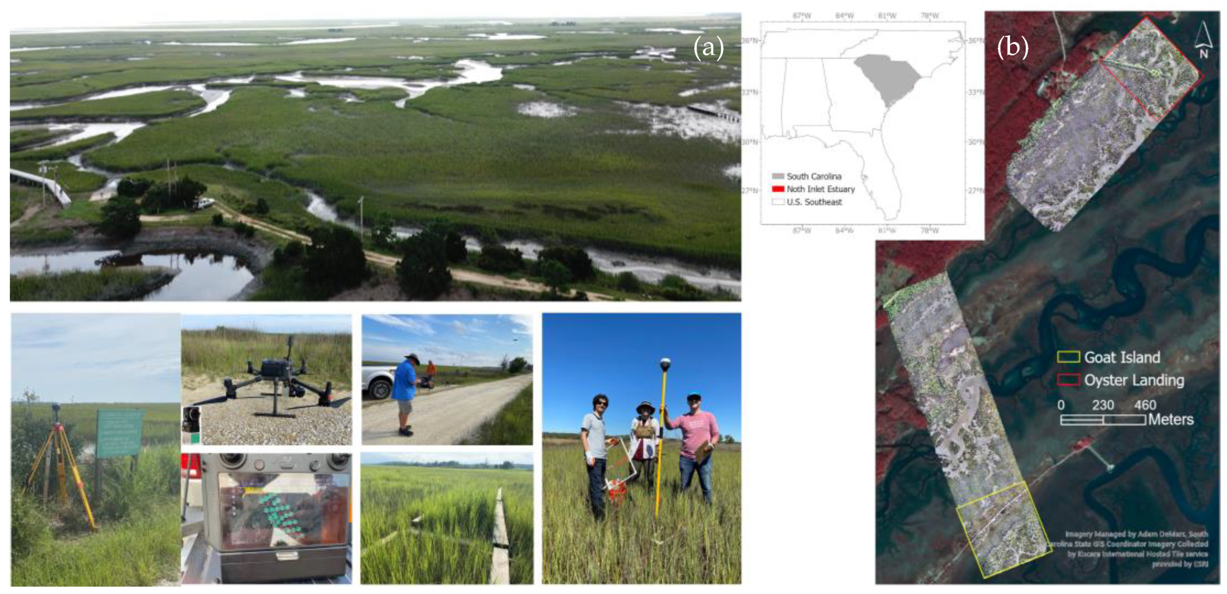
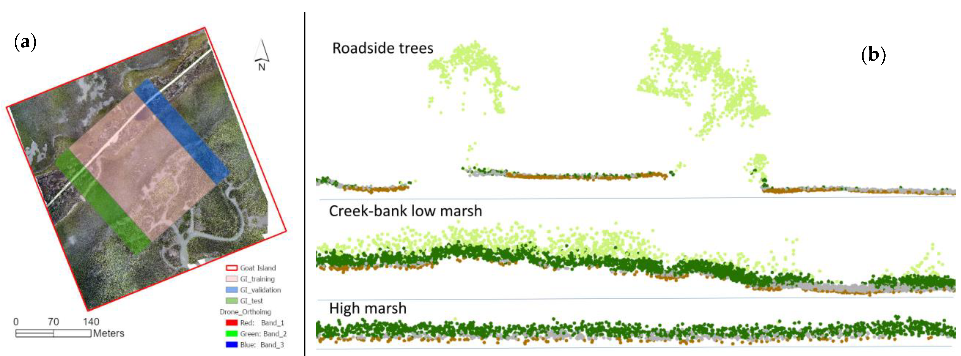
2.1. Study Area and Field Experiment

The North Inlet estuary is located in Georgetown, South Carolina on the U.S. Southeast coast (Figure 1). As an ocean-front pristine estuary, it is characterized by a monoculture of native smooth cordgrass (Spartina alterniflora) growing in the intertidal zone. Regulated by topography and tidal water, the salt marsh wetlands can be roughly divided into two ecological zones. The low marsh zone, dominated by marshes in taller plant forms, is located in the regularly flooded interior estuary. The high marsh zone (in shorter plant forms) lies along the landward margins that have lower inundation times. Figure 1a shows a bird’s-eye drone photo of the estuary. Above the intertidal fringe, maritime forest, shrub/scrub plants, and roadways are visible.

Two subsets in the estuary—Goat Island and Oyster Landing—were selected as our study sites (Figure 1b). A multi-day field experiment was conducted in August–September 2022 to collect drone data and in-field marsh samples in both study sites. On 31 August and 1 September, two drone lidar missions were launched, one at each study site. Each mission had an approximately 30-min flight in the low-tide window. The drone system is a DJI Matrice 300 RTK(SZ DJI Technology Co., Ltd, Shenzhen, China) mounted with a ROCK Robotic R2A (ROCK Robotic, Denver, CO, USA) bundle (that assembles a Lidar sensor (Livox Avia) and a SONY true-color camera (as shown in Figure 1a). The Livox Avia has a compact and lightweight design to be mounted on drones. It features a dual-scanning mode and a Field-of-View angle greater than 70° for improved detection swath and efficiency. In this experiment, we tested its Spirograph scanning mode at Goat Island and the linear scanning mode at Oyster Landing. Flying at an altitude of 80 m, each mission reached a coverage of about 30 ha. The dataset of each mission included the Lidar point cloud at a spacing interval of 3.6 cm and the RGB orthoimage at a pixel size of 3 cm. The purpose of the RGB orthoimage in this experiment was to delineate the non-marsh classes and mask them out of the study. Detailed analysis of the orthoimage was not included.

A total of 36 ground control panels were set up during the two missions. Their (x,y,z) locations were measured with a survey-grade GNSS unit (Emlid Reach base+rover bundle). These ground control points (GCPs) were used to test the positioning accuracies of the collected drone data. For the orthoimages of both strips, a 2nd-order polynomial georeferencing process was performed using the GCPs falling within each strip. For example, the georeferencing of the Goat Island orthoimage with 11 GCPs reached a total RMSE of 5.5 cm in both x and y directions. The orthoimage footprints of both flights are displayed in Figure 1b.

From 21 to 24 September, the research team collected the in-field marsh samples at two experimental sites within the flight footprints (as shown in Figure 1b), hereafter referred to as the Goat Island site and the Oyster Landing site. Both sites support monocultures of Spartina alterniflora. For each field sample, a 0.5 × 0.5 m quadrat was randomly laid in the field, and all marsh plants in the quadrat were clipped and bagged. Before clipping, seven plants in the quadrat were randomly selected, and their natural heights (from the ground to the tip of the plant stand) were measured. The average height served as the sample’s canopy height of the marsh plant, hereafter referred to as marsh height. The plant mass bags were dried for one week in a large-cabinet oven at 70 °C before weighing for dry biomass (g/m²). A total of 40 field samples (marsh height and biomass) at the Goat Island site and 25 samples at the Oyster Landing site were collected.

2.2. Approaches

A multi-step procedure was designed to apply drone Lidar/RGB for 3D marsh mapping in the estuary. With deep learning approaches, three point classes (ground, low vegetation, high vegetation) were classified from the Lidar point cloud. The marsh and non-marsh land covers (mudflat, wrack, forest, and shrub/scrub) were extracted from the orthoimage. A digital terrain model (DTM) was then built from ground points to extract the bare earth topography, followed by a digital surface model (DSM) that was jointly used with DTM to extract marsh height. The drone-extracted marsh height was finally compared with in-field measurements for accuracy assessment and to examine the biophysical condition of marsh vegetation.

2.2.1. Deep Learning for Lidar Point Cloud Classification

The Lidar point cloud was first classified to delineate ground and vegetation points following the LAS Specification (V1.4) standard published by the American Society for Photogrammetry and Remote Sensing [24]. The vegetation points are predominantly marsh points in this estuary. Only two vegetation types were considered: low vegetation and high vegetation. As shown in Figure 1a, maritime forest, roadside trees, and shrubs grow on the upper edge of the land–water interface. Their points were simply counted as high vegetation and were masked out of marsh mapping.

Taking a 4-ha subset at the Goat Island site as the training area (Figure 2a), three point classes—ground, low vegetation, high vegetation—were manually labeled from the vertical point cloud profiles (Figure 2b). Different from trees with large crowns and distinctive canopy structures, marshes are shorter plants in the form of relatively homogeneous grasslands. The visual labeling of training points was heavily weighted on height. The ground points were identified as those at the bottom end of the point cloud, e.g., the dark brown points in Figure 2b. The high vegetation points (light green) were those on the top, revealing apparent canopy structures, for example, the trees and shrubs along the fringe and tall marsh plants in the interior estuary. The low vegetation points were those short plants above ground (dark green). For the points slightly above the ground, it was difficult to visually delineate them, and therefore, they were counted as unassigned (light gray). To reduce uncertainties in our training data, these unassigned points were not used in the training process of the deep learning model.

The training data was split into the training set, validation set, and test set. With the labeled training set, this study utilized a recently developed RandLA-Net model adopted in ArcGIS Pro [23], which is an efficient neural architecture to perform semantic segmentation of large-scale point cloud based on the principles of simple random sampling and local feature aggregation [25,26]. To reduce uncertainties, the manually labeled training set was fed into the RandLA-Net for initial training. The classified points were refined via visual interpretation to finalize the training dataset. The validation set was applied during the RandLA-Net training to evaluate the model performance. With the trained RandLA-Net, the full strip of Lidar point cloud was classified into ground, low vegetation, and high vegetation. Finally, the test set was used to conduct an independent accuracy assessment of the trained model. For each class, model performances were evaluated with the following metrics that have been commonly used in machine learning [27]:

$$\begin{gathered} Precision=\frac{TP}{TP+FP} \\ Recall=\frac{TP}{TP+FN} \\ {F}_1=\frac{2}{\frac{1}{precision}+\frac{1}{recall}} \end{gathered}$$

(1)

where TP, FP, TN, and FN are class-specific measurements: TP (true positive) represents the number of points in a class to be correctly identified as this class; FP (false positive) is the number of points incorrectly identified as this class; TN (true negative) is the number of points that are not this class but are correctly identified; and FN (false negative) is the number of points that are not in this class but are incorrectly identified as this class.

The three evaluation metrics in Equation (1) are class-specific. Precision measures the overestimation and Recall measures the omission of a class. The $F_1$ score is a weighted index of the Precision and Recall metrics to measure the overall performance for this specific class. All three metrics reach the best value at 1.0 and the worst at 0.0. Additionally, an overall accuracy was calculated in this study. It is based on the error matrix in conventional remote sensing, measuring the correctly classified points of all classes against total training samples. Similarly, it has a range of [0.0, 1.0]. An overall accuracy close to 1.0 indicates good performance of the model.

2.2.2. Deep Learning for Orthoimage Classification

Only marsh fields were considered in this study. The orthoimage from the Lidar/RGB bundle was used to mask out the non-marsh areas. Marsh fields include the class types of marsh plants, mudflats, oyster reefs, and water channels. Non-marsh areas include maritime forest, shrub/scrub plants, and roadways on the fringe. To mask out these non-marsh areas, we also performed deep learning classification of the orthoimage. A popular U-Net model adopted in ArcGIS Pro 3.1 was applied to extract the abovementioned classes. The U-Net is an encoder-decoder segmentation network that has been widely accepted for its high efficiency and accuracy in high-resolution image classification [28]. The ultra-fine resolution (3 cm) of the orthoimage allows us to collect the training polygons of each class via visual interpretation. Each class included 10–15 training polygons in the same training area as the Lidar point cloud. After training, the U-Net model was applied to the full-strip orthoimage. The U-Net class map served as a mask; only the marsh fields (marsh vegetation and mudflat/reef) were used for marsh mapping from the Lidar point cloud.

2.2.3. Extracting Bare Earth Surface and Marsh Height

The Digital Surface Model (DSM) and Digital Terrain Model (DTM) were extracted from the classified Lidar point cloud. The DSM surface represents the elevation of marsh vegetation above the datum. Given the Lidar point cloud at a 3.6 cm spacing, a 10 × 10 cm grid size was used to build the raster surface. The grid value was the maximal z-value of all points in this grid. The DTM surface represents the elevation of the bare earth surface in the estuary. It was spatially interpolated from the classified ground points using the triangulated irregular network approach and was exported as a raster surface at a 10 × 10 cm grid size.

With the DSM and DTM raster surfaces, marsh height at each 10 × 10 cm grid can be simply calculated in a canopy height model [29]:

H_marsh = DSM − DTM

(2)

With the 65 marsh samples collected in this experiment, the Lidar-extracted marsh height was statistically compared with the in-field measurements at both experimental sites. To determine the Lidar-extracted marsh height at a sampled location, all pixels in a 3 × 3 window (centered at the sample) were averaged on the marsh height map.

3. Results and Discussion

3.1. Characteristics of Drone Lidar Point Cloud

The drone Lidar point cloud in this experiment reached a spacing of 3.6 cm. At the Goat Island site, its average point density was 771 points per square meter. At such a high density, it sufficiently picked up the morphologic features of marsh plants. As marked in Figure 3(a1), one example is the fertilized marsh plots in the Goat Island high marsh that have been managed as part of an NSF-funded Long-Term Research in Environmental Biology (LTREB) project [30]. Distributed along the boardwalks, these square plots (Figure 3(b1)) showed distinctively taller point clouds than those naturally grown, shorter marsh plants in the field. In a low marsh field in the interior estuary (Figure 3(a2)), drone Lidar identified the tall plants along creek banks, revealing dramatic height dynamics of grasses in the field (Figure 3(b2)).

In comparison, the commonly utilized USGS airborne Lidar has only a 63.9 cm spacing interval with a density of 2.43 points per square meter at the Goat Island site. As shown in Figure 3(c1,c2), although the USGS airborne Lidar also visually depicts the fertilized marsh plots, the point numbers of these plots are limited, only containing a few points in each plot. In the low marsh, marsh height was not well detected (Figure 3(c2)). Figure 3 reveals the advantage of drone Lidar over the sparse USGS airborne Lidar point cloud for marsh height measurement.

The z-value accuracies of the drone Lidar point cloud were evaluated against the survey-grade GNSS measures at ground control targets (Figure 4). A total of 36 GCPs were collected within the two flight strips: 6 at Goat Island, 6 at Oyster Landing, 6 by the vender during the flights, and 16 permanently installed by other research projects monitored by NOAA North Inlet-Winyah Bay National Estuarine Research Reserve (NIWB NERR). At each GCP, a ground control target was laid on the ground (bare earth), and its central position was measured with the GNSS. Figure 4a demonstrates the Lidar points collected at an example ground control target. The Lidar point closest to the target center was selected as the Lidar-collected position of this GCP. With the 36 GCPs, the root-mean-square error (RMSE) of bare earth elevation was 5.55 cm (Figure 4b).

3.2. Deep Learning Classification of Lidar Point Cloud

3.2.1. RandLA-Net Accuracy Assessment

The truthing datasets of three point classes at the Goat Island site are listed in

Table 1. The truthing datasets of Lidar point cloud and the RandLA-Net model performance. The training area is located at the Goat Island site.

Class	Training Set (2.66 ha)		Validation Set (0.59 ha)			Test Set (0.65 ha)
	# of Points	Percent	Precision	Recall	${\mathit{F}}_1$ Score	Precision	Recall	${\mathit{F}}_1$ Score
Ground	2,656,130	8.99%	0.873	0.885	0.879	0.917	0.858	0.886
Low vegetation	10,537,971	35.65%	0.957	0.782	0.860	0.928	0.759	0.835
High Vegetation	5,209,755	17.62%	0.678	0.971	0.798	0.685	0.974	0.804
Unassigned	11,157,757	37.74%	/	/	/	/	/	/
Overall accuracy			0.844			0.834

. The RandLA-Net model was trained in 15 epochs at a batch size of 4 blocks with a block diameter of 4 m. Of all the Lidar points in the 4-ha training area (approximately 30 million points), about 62.3% were manually identified as the truthing points of ground, low vegetation, and high vegetation. Other points located in between ground and vegetation (as shown in the example profiles in Figure 2) were left unassigned and not used in the training process.

The truthing points were fed to the RandLA-Net model, splitting into 2/3 as the training set, 1/6 as the validation set, and 1/6 as the test set (Table 1). The accuracy metrics from the validation set and test set achieved similar results. Among the three point classes, the ground had stably high accuracies of precision, recall, and the $F_1$ scores (0.86–0.89), indicating the validity of extracting bare earth surfaces from the ground points. Among the two vegetation classes, low vegetation had a high precision of 0.93–0.96 (low overestimation), while high vegetation had a high recall of 0.97 (low omission). High vegetation points were correctly classified as such. The points at the lower canopy turned out to be misclassified in the two vegetation classes. Nevertheless, the $F_1$ scores of 0.80–0.86 for both vegetation classes indicated a reasonable classification of vegetation points. The overall accuracies of 0.83–0.84 in Table 1 reveal a valid deep learning process for drone Lidar point cloud classification.

3.2.2. RandLA-Net Extracted Point Classes

Three point classes (ground, low vegetation, and high vegetation) were extracted from the RandLA-Net model. Figure 5 takes the Goat Island site as an example to demonstrate the classification performance. Aside from some trees growing along the roadway, the point cloud had a relatively low elevation above mean sea level and a flat landscape (Figure 5a). The class map (Figure 5b) fairly reflects the marsh distribution in the estuary. Interestingly, the classified drone Lidar point cloud in Figure 5b reveals a distinctive line between low marsh and high marsh in the estuary. The low marsh dominates the interior estuary with tall plants, which were successfully classified as high vegetation (in light green color). As shown in the right profile in Figure 5, the points below the taller canopy were classified as low vegetation (dark green). In the left profile, trees were distinctively identified; the landward high marsh (close to the road) has shorter plants and was classified as low vegetation. Both profiles revealed that ground points (dark brown) occupied the bottom of the cloud point.

After removing the vegetation points, the ground-only point cloud reflects the bare earth topography of the estuary (Figure 5c). Transiting from the road to the interior estuary, the marsh field has a gently sloping elevation surface. There is a clear delineation around the seawater margin (elevation = 0 m). The bare earth surface in the interior estuary is close to or below mean sea level and shows a dark blue color, while the surface further away from the tidal channels has higher elevation in a light blue color. This pattern generally agrees with the delineation between high marsh and low marsh in the class map (Figure 5b). The ground-only point cloud was used to extract DTM in the next section.

3.3. Bare Earth Surface and Marsh Mapping

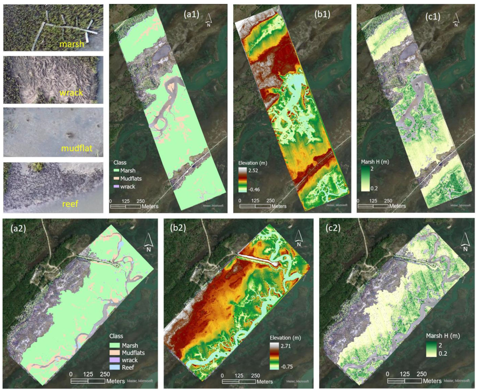
3.3.1. Marsh/Non-Marsh Distribution

The marsh/non-marsh classes of the two strips were extracted from the orthoimages with the U-Net deep learning. The land cover classification was not the focus of this study, and therefore, further assessment was not included in this article. After classification, all class polygons were visually interpreted and modified based on the 3-cm orthoimage to correct any misclassification. For non-marsh classes, similar distributions were observed on both strips: Goat Island (Figure 6(a1)) and Oyster Landing (Figure 6(a2)). Maritime forest covers the landward fringe, and some isolated trees and shrub plants (supratidal upland) grow along the road crossing the estuary. Zones with relatively high elevation support emergent wetlands defined as supratidal haline habitats in the National Wetland Inventory database [31]. Plant species growing in these zones (e.g., Juncus roemerianus, Spartina patens, Distichlis spicata, Salicornia spp.) differ morphologically from the regularly flooded intertidal marsh species (predominantly Spartina alterniflora in the North Inlet estuary). These zones were not considered in this study. Tidal channels were also masked out of the marsh maps.

The marsh fields in the study area are composed of four classes: marsh plants, mudflats, wrack patches, and oyster reefs. Their visual appearances are demonstrated in a few orthoimage subsets in the top left of Figure 6. Among these four classes, a total of 208 polygons were extracted from the Goat Island strip (Figure 6(a1)) and 378 polygons from the Oyster Landing strip (Figure 6(a2)). Drone Lidar point data in these polygons were analyzed.

3.3.2. Bare Earth Surface and Marsh Height

The bare earth surfaces of the two strips (Figure 6(b1,b2)) extracted from the ground points reflected variations in elevation. The maritime forest and emergent wetlands grow on higher topography (higher than 2 m in forests). The intertidal marsh fields have lower elevations that gradually decrease to mean sea level. Lidar point cloud is not available on water surfaces. The topography of tidal channels was calculated from spatial interpolation, which was as low as −0.45 m at Goat Island and −0.75 m at Oyster Landing.

The digital surface model at a 0.1 m grid size was extracted from the points with the maximal height at each grid. In the classified marshes, the marsh height maps at a 0.1 m grid size were thus extracted for both strips (Figure 6(c1,c2)). As expected, high marsh plants in the landward estuary are much shorter in stature, while low marsh plants in the interior estuary are taller. Both marsh height maps reveal a clear distinction between the two marsh types. Spartina alterniflora plants here rarely exceed 2 m.

Be aware of the phenomenon of apparent linear patterns at Oyster Landing (Figure 6(c2)) that was not observed at Goat Island (Figure 6(c1)). This was attributed to different scanning modes between the two flight missions. The Livox Avia adopts multi-linear high-speed laser technologies (http://livoxtech.com/avia, accessed on 9 November 2023). At Goat Island, a non-repetitive, circular (spirograph) scanning mode was utilized to increase the coverage area ratio, which detected more object details within Lidar’s field of view at the expense of more time consumption. At Oyster Landing, a repetitive, linear scanning mode was utilized in order to take advantage of time efficiency. Apparently, the linear scanning (Figure 6(c2)) resulted in higher confusion between the flight lines than the spirograph scanning, especially in low marsh zones with taller plants and more complicated canopy structures. This observation may help the operational deployment of drone Lidar in coastal monitoring.

A 3D view of the marsh height map at the Goat Island site revealed the spatial variations of marsh vegetation stature (Figure 7). Three field pictures are included on top of the figure: a high marsh field with a field scientist fixing the boardwalk (left), an LTREB-managed marsh plot (middle), and a low marsh field with tall plants along the creek bank (right). In alignment with these field pictures, the high marsh on the left of the map was apparently shorter than the low marsh close to the creek bank to the right. The LTREB long-term fertilized marsh plots stood out clearly in the low marsh field. The boardwalks and a weather monitoring pole (in the top right) were depicted from drone Lidar data.

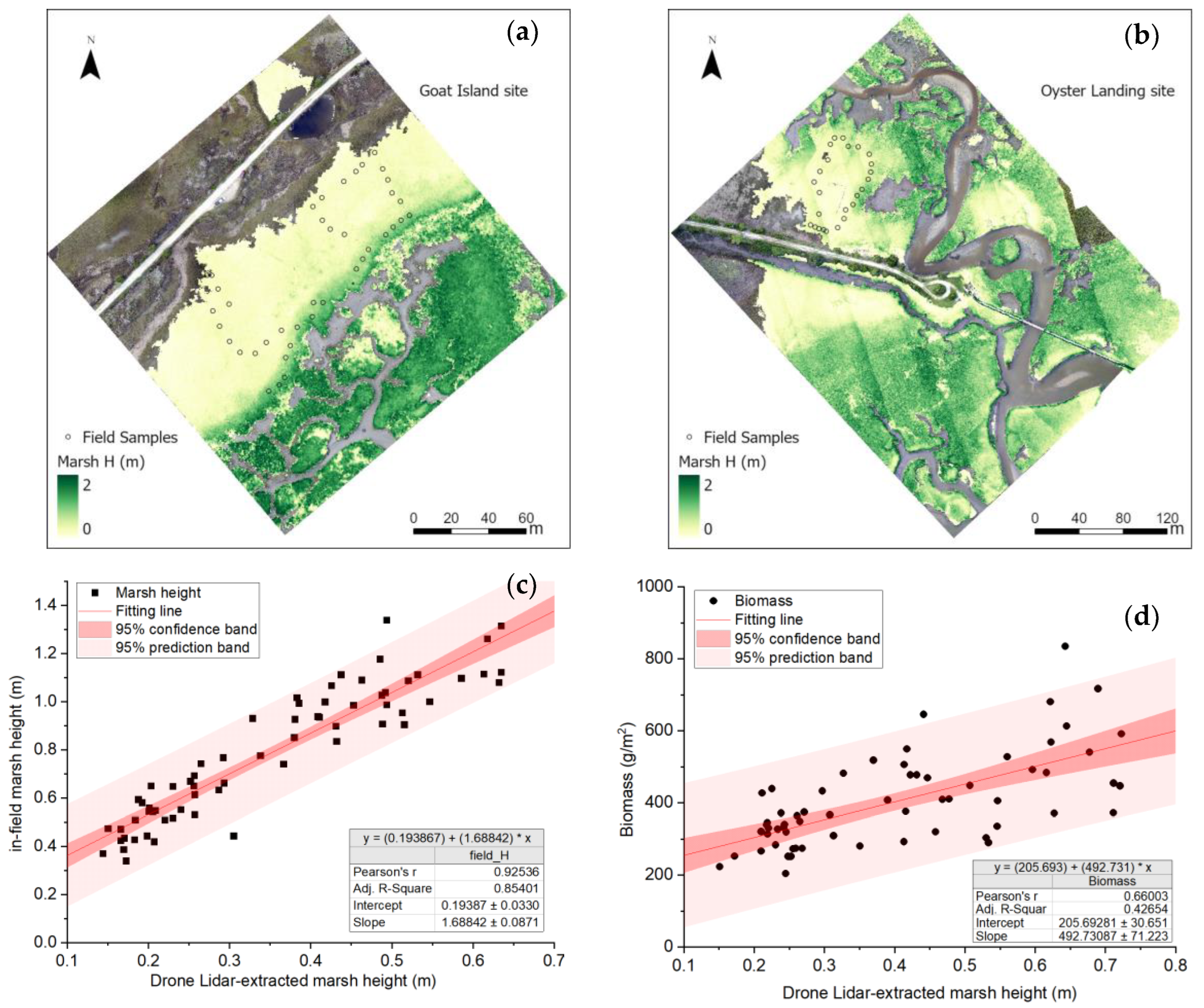
3.4. Comparison between Lidar-Extracted and Field Measurements

The Lidar-extracted marsh height was compared with the in-field measurements at two experimental sites with the locations of 65 field samples marked (Figure 8). The Goat Island site (Figure 8a) has an apparent transition from an emergent, supratidal wetland to an intertidal marsh wetland. Only marsh fields were mapped. There was a clear delineation between the two marsh types: high marsh (light yellow) in the northwest and low marsh (green) along creek banks in the interior estuary. The Oyster Landing site (Figure 8b) did not show a sharp split but was also characterized by short plants close to the roadway and tall plants close to tidal channels.

In the scatterplot of the 65 samples (Figure 8c), the Lidar-extracted marsh heights are unanimously lower than the field-measured marsh heights. However, the plot reveals a significant linear relationship between the two with Pearson’s r = 0.925. As a result, the Lidar-extracted marsh height can be simply adjusted according to the linear regression. Among the 65 samples, only two measurements fell outside of the 95% confidence envelope (95% prediction band). The confidence band in the figure represents the 95% envelope in which the best-fit line falls. Applying the regression equation in Figure 8c, the adjusted Lidar-extracted marsh height reached an RMSE of 0.12 cm when compared with the in-field marsh height at the 65 samples.

Marsh height was closely related to standing marsh biomass in the estuary. In Figure 8d, a linear relationship between the Lidar-extracted canopy height and the sampled dry standing biomass is observed with Pearson’s r = 0.66. Only two out of 65 samples fell outside of the 95% confidence envelope. Both linear relationships (Figure 8c,d) were statistically significant in a student’s t test (p < 0.05). The larger residuals (wider bandwidth of the 95% prediction band) indicated that other marsh parameters may contribute to the measurement of marsh biomass, which will be investigated in future research.

3.5. Further Thoughts: Drone Lidar for Intertidal Ecosystem Monitoring

Quantitative marsh mapping in intertidal zones has been challenging due to the difficulties in accessing the wetlands for field experiments and the short low-tide window for satellite remote sensing observations. Airborne Lidar has proven effective in terrestrial landscape mapping, but its applications in intertidal ecosystems have not achieved acceptable accuracies [7,9,17]. As visually compared in Figure 3, the commonly utilized USGS airborne Lidar point cloud only contains 2 to 3 points per square meter in the experimental site of this study. Especially in high marsh habitats with short, sparse plants, it is difficult to delineate ground and vegetation points. There are basically no Lidar returns on water surfaces. Airborne Lidar application is further impacted by the frequent tidal flooding in marsh fields.

This experimental study reveals the feasibility of drone Lidar for extracting bare earth surfaces and 3D marshes in intertidal estuaries. Flying at 80 m above ground, drone Lidar (Livox Avia in this experiment) is capable of collecting 600–800 points per square meter, reaching a spacing interval of cm- instead of m-scales typical of the USGS airborne Lidar. With deep learning technologies of mass points, ground points and vegetation points can be effectively identified, bare earth surfaces extracted, and marsh height calculated at cm-scales. Although the Lidar-extracted marsh canopy heights are lower than the in-field measurements, their strong linear relationship allows the adjustment for real-world marsh height mapping from drone Lidar. The linear relationship between the model-derived marsh canopy height and the sampled aboveground dry biomass also supports the utility of drone Lidar for marsh biomass estimation across the estuary.

Aside from marsh height, the drone Lidar point cloud may also be further analyzed to extract marsh stem density. It has been observed in past studies [9] that airborne Lidar received predominantly single returns in the intertidal estuary. The same phenomenon from drone Lidar was observed in this experiment. Except for the forests and roadside trees that could receive 2 to 3 returns, only single returns were available in the vast area of the estuary. The single-return features limit the cloud point’s capability to describe the canopy structure of marsh plants. However, it may reveal interesting information about stem density that, together with canopy height, could play an important role in quantifying marsh biomass. Future efforts will be made to further investigate the feasibility of extracting marsh density from drone Lidar point clouds.

Be aware of the environmental limitations encountered during this experiment. Due to the physical difficulty in accessing field sites, sample collections were limited largely to high marsh habitats closer to the roadways (as marked in Figure 8a,b), with a few exceptional samples along creek banks. Therefore, marsh canopy height and biomass in the sample set turned out to be low; samples from low marsh habitats in the interior estuary were underrepresented. If more samples in low marshes become available in the future, the drone Lidar-extracted marsh height may be better assessed for its validity as an indicator of marsh biophysical properties on the coast. Another limitation of drone Lidar deployment in the estuary is the short low-tide window. Using the North Inlet Estuary in this study as an example, it experiences a tidal change around every six hours, with two low tides and two high tides a day. Only during the short low-tide windows can drone Lidar be deployed to collect point clouds. The low-tide tidal heights also vary significantly depending on the date, ranging from below −1 ft to above 1 ft (referenced to Mean Lower Low Water or MLLW). Therefore, time availability for drone missions is limited, practically less than one hour during a low-tide window. Drone missions have to be well prepared to meet the time window.

This study tested a general procedure of drone Lidar applications in a sequence of lidar data collection, point cloud classification, bare earth surface extraction, and marsh height calculation. Depending on the applied environment, specific considerations may need to be involved for best practices. For example, this experimental study was conducted in a relatively homogeneous marsh environment dominated by the pristine monoculture of Spartina alterniflora. The bare earth topography in the study site was relatively smooth. It sufficiently delineated the ecologically different marsh types (low marsh vs. high marsh) from drone Lidar point clouds. When adopting this procedure for drone Lidar applications in other coastal environments, localized complexities, such as dynamic tidal effects, diverse vegetation species, and changing terrains may be encountered. If long-term, repetitive monitoring is planned, environmental seasonality and vegetation phenology may also need to be considered. Especially the initial steps of this procedure, Lidar point cloud collection and classification, are crucial to the accuracies of bare earth and marsh height extraction. This study found the spirograph scanning mode of the Lidar system had better results than linear scanning in overlaid areas between two flight lines. For point cloud deep learning, the RandLa-Net model achieved an overall accuracy of around 0.84 (the F₁ score of 0.89 for ground points), which was lower than those deep learning classifications based on high-resolution imagery. It was understandable since the point-based training data sets do not have structured shapes as in the imagery. Also, uncertainties in training data collection for deep learning were inevitably introduced when visually identifying the points in the three classes. With new Liar sensors and advanced point cloud deep learning technologies available, the approaches tested in this study could be better adapted for improved 3D terrain monitoring on the coast.

Coastal communities are facing the foremost challenges from accelerating climate change and sea level rise (SLR). The drone Lidar-extracted fine-scale maps of bare earth surfaces and marsh biophysical properties provide essential base information to assess the environmental resilience of coastal ecosystems. Various federal and state efforts have been made to model coastal inundation, e.g., the NOAA Digital Coast “Sea Level Rise Viewer” web mapping tool (https://coast.noaa.gov/digitalcoast/tools/slr.html, accessed on 9 November 2023) that provides a nationwide visual projection of coastal flooding from SLR based on satellite imagery and digital terrain models at 30–1000 m grid sizes. Constrained by data availability and coarse resolutions, current model projections hold significant uncertainties in potential marsh migration corridors. This study indicates that drone Lidar-extracted information may feed current marsh equilibrium and wetland inundation models to better simulate the potential impacts of SLR on shoreline modification and wetland conversion. All this information is crucial for coastal communities on marsh restoration prioritization and coastal development planning to promote a more resilient, sustainable future.

4. Conclusions

With the accelerated sea level rise, fine-scale information of bare earth surfaces and marsh properties is essential for accurate projection of tidal inundation and coastal resilience. This study explored the feasibility of drone Lidar for 3D marsh mapping in an intertidal estuary. Applying the RandLA-Net deep learning model, a multi-step procedure of drone Lidar deployment was established to classify the drone Lidar point cloud and to extract bare earth surface and marsh height at a 10 cm grid size. The primary findings of this experimental study are summarized below:

(1)

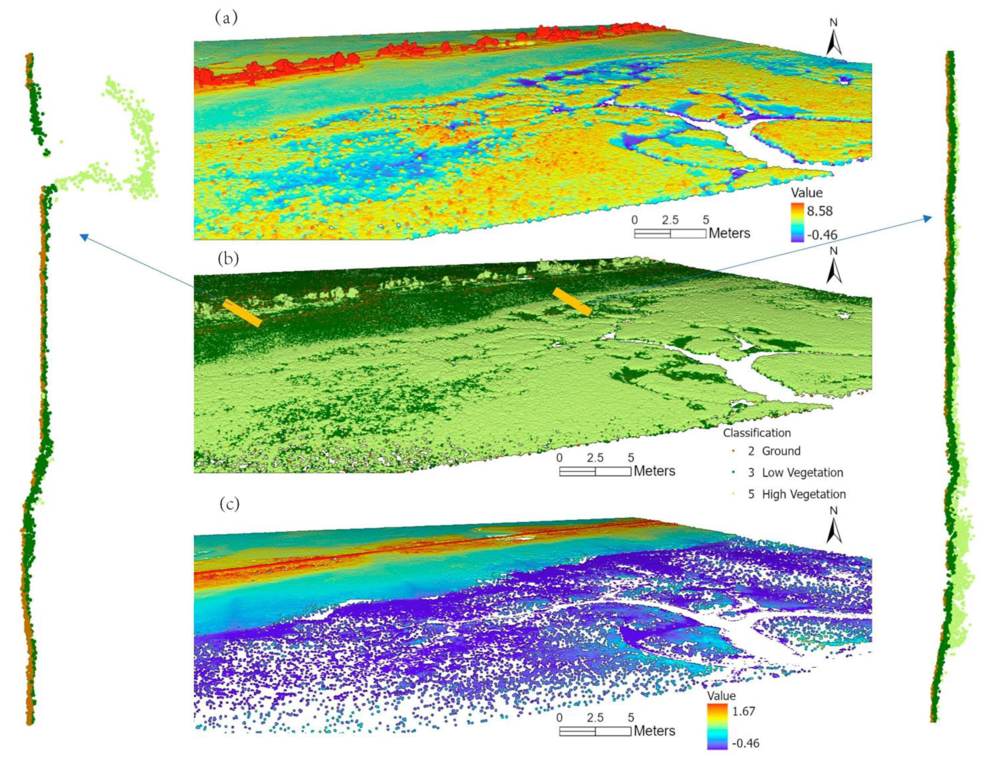
Deep learning classification effectively delineates ground, low vegetation, and high vegetation points in the drone Lidar point cloud at an overall accuracy of around 0.84.

(2)

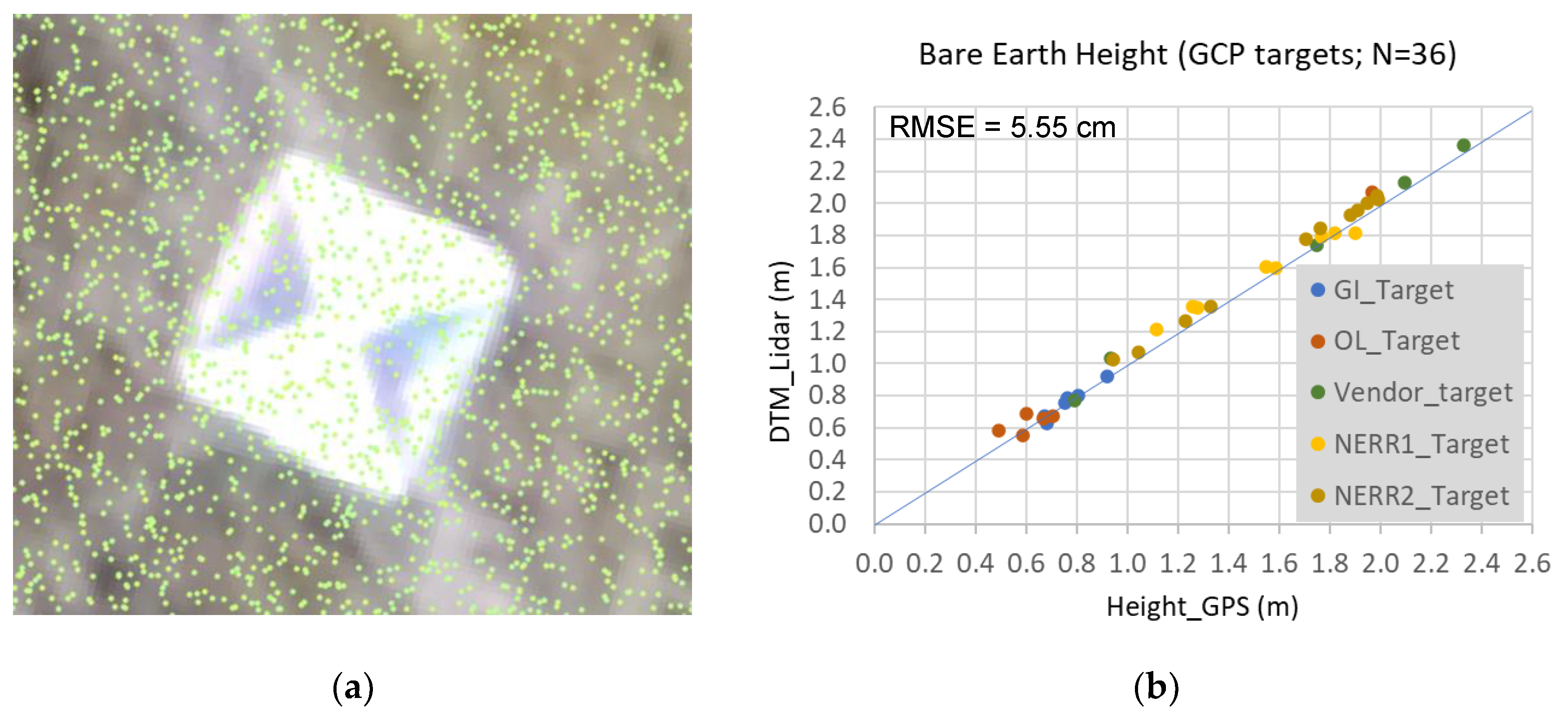
Drone Lidar systems could be utilized to extract centimeter-level bare earth surfaces at a vertical accuracy of 5.55 cm (RMSE) in intertidal zones.

(3)

The drone Lidar-extracted marsh height was lower than the in-field measurements, but they possessed a strong linear relationship (Pearson’s r = 0.93). With the collected 65 samples, the adjusted Lidar-extracted marsh height reached an RMSE of 0.12 cm.

(4)

It is worth mentioning that the classified drone Lidar point cloud fairly delineates the high marsh and low marsh habitats along a gently decreasing topographic gradient in the estuary.

As the ineffectiveness of airborne Lidar in mapping coastal wetlands has been recognized in current literature, this study reveals drone Lidar could be a useful tool for accurate 3D terrain and marsh mapping on the intertidal coast. Future investigation is suggested to explore drone Lidar applications in dynamic coastal environments and in marsh biomass quantification.

References

1. Sanger, D.; Parker, C. Guide to the Salt Marshes and Tidal Creeks of the Southeastern United States; South Carolina Department of Natural Resources: Charleston, SC, USA, 2016; p. 112. [Google Scholar]
2. Sweet, W.V.; Hamlington, B.D.; Kopp, R.E.; Weaver, C.P.; Barnard, P.L.; Bekaert, D.; Brooks, W.; Craghan, M.; Dusek, G.; Frederikse, T.; et al. Global and Regional Sea Level Rise Scenarios for the United States: Updated Mean Projections and Extreme Water Level Probabilities along U.S. Coastlines; NOAA Technical Report NOS 01; NOAA National Ocean Service: Silver Spring, MD, USA, 2022; p. 111. [Google Scholar]
3. U.S. Geological Survey (USGS). USGS Lidar Point Cloud (LPC). 2014. Available online: https://data.usgs.gov/datacatalog/data/USGS:b7e353d2-325f-4fc6-8d95-01254705638a (accessed on 15 September 2023).
4. Wang, C.; Morgan, G.; Hodgson, M.E. sUAS for 3D tree surveying: Comparative experiments on a closed-canopy earthen dam. Forests 2021, 12, 659. [Google Scholar] [CrossRef]
5. Schmid, K.A.; Hadley, B.C.; Wijekoon, N. Vertical accuracy and use of topographic Lidar data in coastal marshes. J. Coast. Res. 2011, 27, 116–132. [Google Scholar] [CrossRef]
6. Hladik, C.; Alber, M. Accuracy assessment and correction of a Lidar-derived salt marsh digital elevation model. Remote Sens. Environ. 2012, 121, 224–235. [Google Scholar] [CrossRef]
7. Amante, C. Estimating coastal digital elevation model uncertainty. J. Coast. Res. 2018, 34, 1382–1397. [Google Scholar] [CrossRef]
8. Medeiros, S.C.; Bobinsky, J.S.; Abdelwahab, K. Locality of topographic ground truth data for salt marsh Lidar DEM elevation bias mitigation. IEEE J. Sel. Top. Appl. Earth Obs. Remote Sens. 2022, 15, 5766–5775. [Google Scholar] [CrossRef]
9. Fernandez-Nunez, M.; Burningham, H.; Zujar, J.O. Improving accuracy of Lidar-derived terrain models for saltmarsh management. J. Coast Conserv. 2017, 21, 209–222. [Google Scholar] [CrossRef]
10. Abeysinghe, T.; Simic Milas, A.; Arend, K.; Hohman, B.; Reil, P.; Gregory, A.; Vázquez-Ortega, A. Mapping invasive Phragmites Australis in the Old Woman CREEK Estuary using UAV remote sensing and machine learning classifiers. Remote Sens. 2019, 11, 1380. [Google Scholar] [CrossRef]
11. Dai, W.; Li, H.; Chen, X.; Xu, F.; Zhou, Z.; Zhang, C. Saltmarsh expansion in response to morphodynamic evolution: Eield observations in the Jiangsu coast using UAV. J. Coast. Res. 2020, 95 (Suppl. S1), 433. [Google Scholar] [CrossRef]
12. Haskins, J.; Endris, C.; Thomsen, A.S.; Gerbl, F.; Fountain, M.C.; Wasson, K. UAV to inform restoration: A case study from a California tidal marsh. Front. Environ. Sci. 2021, 9, 642906. [Google Scholar] [CrossRef]
13. Meng, X.; Shang, N.; Zhang, X.; Li, C.; Zhao, K.; Qiu, X.; Weeks, E. Photogrammetric UAV mapping of terrain under dense coastal vegetation: An object-oriented classification ensemble algorithm for classification and terrain correction. Remote Sens. 2017, 9, 1187. [Google Scholar] [CrossRef]
14. Durgan, S.; Zhang, C.; Duecaster, A. Evaluation and enhancement of unmanned aircraft system photogrammetric data quality for coastal wetlands. GISci. Remote Sens. 2020, 57, 865–881. [Google Scholar] [CrossRef]
15. Pinton, D.; Canestrelli, A.; Wilkinson, B.; Ifju, P.; Ortega, A. A new algorithm for estimating ground elevation and vegetation characteristics in coastal salt marshes from high-resolution UAV-based Lidar point clouds. Earth Surf. Process. Landf. 2020, 45, 3687–3701. [Google Scholar] [CrossRef]
16. Curcio, A.C.; Peralta, G.; Aranda, M.; Barbero, L. Evaluating the performance of high spatial resolution UAV-photogrammetry and UAV-Lidar for salt marshes: The Cádiz Bay study case. Remote Sens. 2022, 14, 3582. [Google Scholar] [CrossRef]
17. Blount, T.; Silvestri, S.; Marani, M.; D’Alpaos, A. Lidar derived salt marsh topography and biomass: Defining accuracy and spatial patterns of uncertainty. Int. Arch. Photogramm. Remote Sens. Spat. Inf. Sci. 2023, XLVIII-1/W1-2023, 57–62. [Google Scholar] [CrossRef]
18. Qi, C.R.; Yi, L.; Su, H.; Guibas, L.J. PointNet++: Deep hierarchical feature learning on point sets in a metric space. In Proceedings of the Advances in Neural Information Processing Systems (NIPS), Long Beach, CA, USA, 4–9 December 2017; Volume 18, pp. 5099–5108. [Google Scholar]
19. Li, Y.; Bu, R.; Sun, M.; Wu, W.; Di, X.; Chen, B. PointCNN: Convolution on X-transformed points. In Proceedings of the 32nd Conference on Neural Information Processing Systems, Montréal, QC, Canada, 3–8 December 2018; pp. 828–838. [Google Scholar]
20. Wang, Y.; Sun, Y.; Liu, Z.; Sarma, S.E.; Bronstein, M.M.; Solomon, J. Dynamic graph CNN for learning on point clouds. ACM Trans. Graph 2019, 38, 1–12. [Google Scholar] [CrossRef]
21. Li, Y.; Ma, L.; Zhong, Z.; Cao, D.; Li, J. TGNet: Geometric graph CNN on 3-D point cloud segmentation. IEEE Trans. Geosci. Remote Sens. 2019, 58, 3588–3600. [Google Scholar] [CrossRef]
22. Diab, A.; Kashef, R.; Shaker, A. Deep learning for Lidar point cloud classification in remote sensing. Sensors 2022, 22, 7868. [Google Scholar] [CrossRef]
23. ESRI. Introduction to Deep Learning and Point Clouds, ArcGIS Pro 3.1. 2023. Available online: https://pro.arcgis.com/en/pro-app/latest/help/data/las-dataset/introduction-to-deep-learning-and-point-clouds.htm (accessed on 15 September 2023).
24. ASPRS. LAS Specification 1.4–R14; Published by the American Society for Photogrammetry and Remote Sensing (ASPRS). 2019. Available online: https://www.asprs.org/wp-content/uploads/2019/03/LAS_1_4_r14.pdf (accessed on 15 September 2023).
25. Hu, Q.; Yang, B.; Xie, L.; Rosa, S.; Guo, Y.; Wang, Z.; Trigoni, N.; Markham, A. RandLA-Net: Efficient semantic segmentation of large-scale point clouds. In Proceedings of the IEEE/CVF Conference on Computer Vision and Pattern Recognition (CVPR), Seattle, WA, USA, 13–19 June 2020; pp. 11108–11117. [Google Scholar]
26. Ma, Z.; Li, J.; Liu, J.; Zeng, Y.; Wan, Y.; Zhang, J. An improved RandLa-Net algorithm incorporated with NDT for automatic classification and extraction of raw point cloud data. Electronics 2022, 11, 2795. [Google Scholar] [CrossRef]
27. Huang, X.; Wang, C.; Li, Z.; Ning, H. A visual-textual fused approach to automated tagging of flood-related tweets during a flood event. Int. J. Digit. Earth 2018, 11, 1248–1264. [Google Scholar]
28. Pashaei, M.; Kamangir, H.; Starek, M.J.; Tissot, P. Review and evaluation of deep learning architectures for efficient land cover mapping with UAS hyper-spatial imagery: A case study over a wetland. Remote Sens. 2020, 12, 959. [Google Scholar] [CrossRef]
29. Mielcarek, M.; Stereńczak, K.; Khosravipour, A. Testing and evaluating different LiDAR-derived canopy height model generation methods for tree height estimation. Int. J. Appl. Earth Obs. Geoinf. 2018, 71, 132–143. [Google Scholar] [CrossRef]
30. Morris, J.; Sundberg, K. LTREB: Aboveground Biomass, Plant Density, Annual Aboveground Productivity, and Plant Heights in Control and Fertilized Plots in a Spartina Alterniflora-Dominated Salt Marsh, North Inlet, Georgetown, SC: 1984–2020. Ver. 5. Environmental Data Initiative. 2021. Available online: https://portal.edirepository.org/nis/mapbrowse?packageid=edi.135.5 (accessed on 15 September 2023).
31. U.S. Fish and Wildlife Service (FWS). The National Wetlands Inventory. 2018. Available online: https://data.nal.usda.gov/dataset/national-wetlands-inventory (accessed on 15 September 2023).
Figure 1. An oblique drone image for bird’s-eye view of the North Inlet estuary (a) and two drone flight footprints (b). The field pictures in the lower left demonstrate the instruments (drones, sensors, GNSS) deployed during flight and field sampling.
Sustainability 15 15823 g001
Figure 2. The training area for Lidar deep learning (a) and three example point profiles at selected locations (b). Three point classes are explored: ground (dark brown), low vegetation (green), and high vegetation (light green). The unassigned points are light grey.
Sustainability 15 15823 g002
Figure 3. Example marsh fields at Goat Island. Their drone orthoimages (a) and point clouds of drone Lidar (b) and USGS airborne Lidar (c) are visually compared. The top row is a high marsh (a1c1); the bottom row is a low marsh along creek bank (a2c2).
Sustainability 15 15823 g003
Figure 4. An example ground control target (a) and the scatterplot to evaluate the vertical accuracies of drone Lidar point cloud at 36 GCPs (b).
Sustainability 15 15823 g004
Figure 5. The 3D view of drone Lidar point cloud at Goat Island: raw point cloud in a color scheme of elevation (a), the classified point cloud (b), and the ground-only point cloud in elevation (c). Also displayed are the vertical profiles of a roadside transect (left) and a creek bank transect (right) at a one-foot width.
Sustainability 15 15823 g005
Figure 6. The extracted marsh/non-marsh class (a1,a2), bare earth surface (b1,b2), and marsh height (c1,c2) maps of the two flight strips: Goat Island (top) and Oyster Landing (bottom). Example orthoimages of the four classes in marsh fields are demonstrated in the top left.
Sustainability 15 15823 g006
Figure 7. A 3D view of marsh height distribution at the Goat Island site. The three field pictures on the top are high marsh (left), fertilized marsh plot (middle, marked in red ellipse), and creek-bank low marsh (right), respectively. The marsh plot is also marked in the marsh height map.
Sustainability 15 15823 g007
Figure 8. Sample points on the marsh height maps at Goat Island (a) and Oyster Landing (b) experimental sites. Also in the figure are the comparisons between the Lidar-extracted and field-measured marsh height (c) and biomass (d) of the 65 samples.
Sustainability 15 15823 g008