Abstract
As cities expand, residents are experiencing increasing commuting distances and a growing trend of job–housing separation, which is often associated with traffic congestion, inefficiency in commuting, and air pollution. In the process of studying the urban job–housing balance, most scholars focus on exploring socio-economic indicators, overlooking the more fundamental characteristics—the geographical features and barriers of the city. This paper delves into the intricate dynamics of the job–housing balance in urban areas, focusing on the city of Boston, characterized by its unique geographic and demographic tapestry. Through the job–housing distribution data of over 3 million residents in Boston and a measurement of spatial proximity to natural barriers, we explore the impact of geographic barriers on residential and employment distributions. Our findings reveal a pronounced divergence in employees’ preferences for job and housing locations, with tracts in the margin areas showing higher aggregation of job distributions and those near geographic barriers exhibiting a low job–housing ratio (JHR) index. Using regression models, our study determined that for every 1% increase in proximity to the Atlantic Ocean on Boston’s right side, job opportunities would decrease by 0.102%, and the JHR would experience a reduction of 0.246%. Our findings prove the importance of the effects of natural barriers on the job–housing balance and provide insights into traffic congestion and the uneven distribution of housing supply prices and have significant implications for urban planning and policy formulation, particularly in coastal cities. By exploring the multifaceted nature of urban residency and employment and the role of geographical constraints therein, this paper contributes valuable perspectives for fostering equitable and sustainable urban development.
1. Introduction
The continually increasing commuting times and escalating job–housing separation have become significant obstacles to achieving sustainable urban development. Commuting is one of the most critical activities in the daily lives of urban residents, playing a crucial role in realizing individual labor values, fostering the formation of social networks, and ensuring the smooth operation of the urban economy [1,2]. However, the continuous expansion of cities and the intensifying trend of motorization have led to a series of social problems, such as the lagging industrialization of suburbs, the monotony of land use functions, and the inadequacy of public transport infrastructure, resulting in extended commuting times and serious job–housing separation [3,4,5,6].
The most direct cause of job–housing separation is the increasing reliance on private vehicles. According to data from the Traffic Management Bureau of the Ministry of Public Security [7], by the end of 2019, the number of vehicles in China had reached 260 million, with 66 cities having more than one million vehicles, and the number of private cars (small and micro passenger cars for personal use) had reached 207 million. The rapidly rising number of private cars reflects the ever-increasing transport demands of urban residents and is also an important reason for the gradual intensification of urban traffic congestion. In December 2020, the China Academy of Urban Planning and Design released the “National Major Cities Commuting Time Consumption Monitoring Report” [8], which reported the commuting indicators of 36 key cities: average one-way commuting time consumption, the proportion of commuters with one-way time consumption within 45 min, and the proportion of commuters with one-way time consumption exceeding 60 min. The report revealed that among the 36 cities, over 10 million people had commuting times exceeding 60 min, accounting for 13% of the commuting population. The average commuting distance in the four mega-cities (Beijing, Shanghai, Guangzhou, Shenzhen) was as high as 9.3 km.
The growing distance between job and residential locations, coupled with the consequent escalation in commuting duration, is indicative of severe adverse effects on the daily lives of commuters. Lengthy commutes not only increase the commuting expenses of residents but also elevate the incidence of diseases such as obesity and hypertension, and the prevalence of psychological disorders like anxiety and depression [9], ultimately diminishing the well-being of urban inhabitants. Beyond individual impacts, a job–housing imbalance also gives rise to severe societal issues, including widening income disparities, aggregating traffic congestion, and exacerbating social inequality [10,11]; concurrently, the lengthy commuting distances also amplify energy consumption and intensify urban environmental pollution. In 2018, the total emissions of the four pollutants from motor vehicles in China were preliminarily calculated to be 40.653 million tons, including carbon monoxide (), hydrocarbons (), nitrogen oxides (), and particulate matter (), becoming the primary source of urban air pollution, seriously endangering human respiratory and nervous systems [12,13].
Exploring the key factors that influence the job–housing distribution of urban residents has become a research priority for shortening commuters’ travel distances and reducing social inequality [14,15]. Urban economic theories have been widely used to explain the relationship between job–housing separation and urban form. Alonso’s influential work on spatial structure [16] found the phenomenon that high-income residents are willing to endure longer commutes for the trade-off of a better living environment and larger living space in the edge of cities, whereas low-income households tend to aggregate in old housing near job centers to save on commuting costs. Muth [17] further improved Alonso’s concentric model and pointed out that job–housing choices and urban form are shaped by income levels and housing prices, which first revealed the connection between urban spatial dynamics and property values. Subsequent research by Mills [18] expanded on these theories, illustrating how job–housing imbalances can be exacerbated by the decentralization of industries. Mills also pointed that increasing investment on urban transportation infrastructure would have a significant effect on optimizing the job–housing distribution pattern, which was widely confirmed by recent studies [4]. Recent studies have begun to focus on the nuanced role of property values within this discourse [19,20]. They provide empirical evidence suggesting that escalating property values in urban centers drive the working population to outlying areas, disrupting the job–housing balance, and creating a commuter economy. These studies have deepened urban managers’ understanding of the relationship between the urban economy and job–housing imbalance. However, socioeconomic factors are often challenging to assess accurately and exhibit high interdependence, leading to considerable uncertainty in the relationship between socioeconomic factors and people’s job–housing choices.
Besides socioeconomic factors, recent researches have started to focus on the more fundamental factors impacting the job–housing imbalance—urban constraints or urban barriers. Harari [21] found that in India, cities with fewer geographic barriers tend to have more compact urban forms. This compactness typically results in faster population growth, higher productivity, and improved quality of life. Complex geographic environments can lead to less compact urban forms and result in larger income disparities and lower productivity within cities, a finding consistent with Duque’s [22] discoveries in Latin America. Harari also pointed out that a complex geographic environment might imply longer commuting times. Angel [23] assessed the impact of urban shape on socio-economic indicators, pointing out that commuting distances are jointly influenced by population density and compactness. However, the mechanism of this impact and the magnitude of its influence are challenging to measure. Saiz [24] finds that geographic barriers significantly affect the spatial distribution of urban commuters by influencing the housing supply and job–housing balance. Ahlfeldt [25] identified the mechanism between the available developable land area in a city and commuting costs; the smaller the area of developable land in a city, the farther its urban boundary will be from the city center as the population increases, leading to greater commuting distances and costs.
Whether the presence of urban geographical barriers affects the distribution of jobs and housing among urban residents and the balance of jobs and housing still lacks effective evidence. Researching the mechanism by which geographical barriers affect the balance of jobs and housing and urban congestion is of significant importance for achieving sustainable urban development. To address this issue, this paper takes Boston, one of the most congested coastal cities in the United States, as the research object and explores the correlation between the distribution of jobs and housing among Boston residents and its geographical terrain features. First, this paper calculates the spatial distribution of geographical barriers in the Boston area based on land-use data as the basic data for this paper. Secondly, this paper obtained job and housing spatial distribution data for over 3 million residents in the Boston area in 2020, and based on this data, calculated neighborhood-level indicators to assess the balance of job and housing distribution. Then, we introduced various neighborhood-level attribute information such as road network length, population, housing quantity, etc., as control variables for subsequent regression models, and calculated the accessibility and spatial distance between neighborhoods and geographical barriers as our variables of interest in subsequent regression models. Finally, through a spatial econometric model, we explored the association between the job–housing balance index and the distribution of geographical barriers.
The results show that the presence of geographical barriers has a negative impact on the distribution of job opportunities. Through regression models, we found that for every 1% closer to the Atlantic Ocean on the right side of Boston, there would be a 0.102% decrease in job opportunities and a 0.246% reduction in the job–housing ratio (JHR). Although areas close to geographical barriers tend to have higher amenities and attract residents to live nearby, the job–housing balance issue in these areas is often more significant compared to the decrease in job opportunities. During our research on geographical barriers and job–housing balance, we controlled for the distance of tracts to the city center and some socio-economic indicators, such as population, housing stock, road network density, etc. We found that developed road networks and ample available land can to some extent increase companies’ willingness to provide job opportunities, thereby alleviating the negative impact caused by the presence of geographical barriers. This paper’s research preliminarily confirms the impact of geographical barriers on residents’ job–housing distribution, helps to explain the potential reasons for traffic congestion and uneven distribution of housing supply prices in coastal cities from a mechanistic perspective, and aids policymakers in proposing regional transportation optimization policies, housing supply policies, and employment improvement measures at a macro level (especially for coastal cities).
2. Study Area and Data Sources
2.1. Study Area
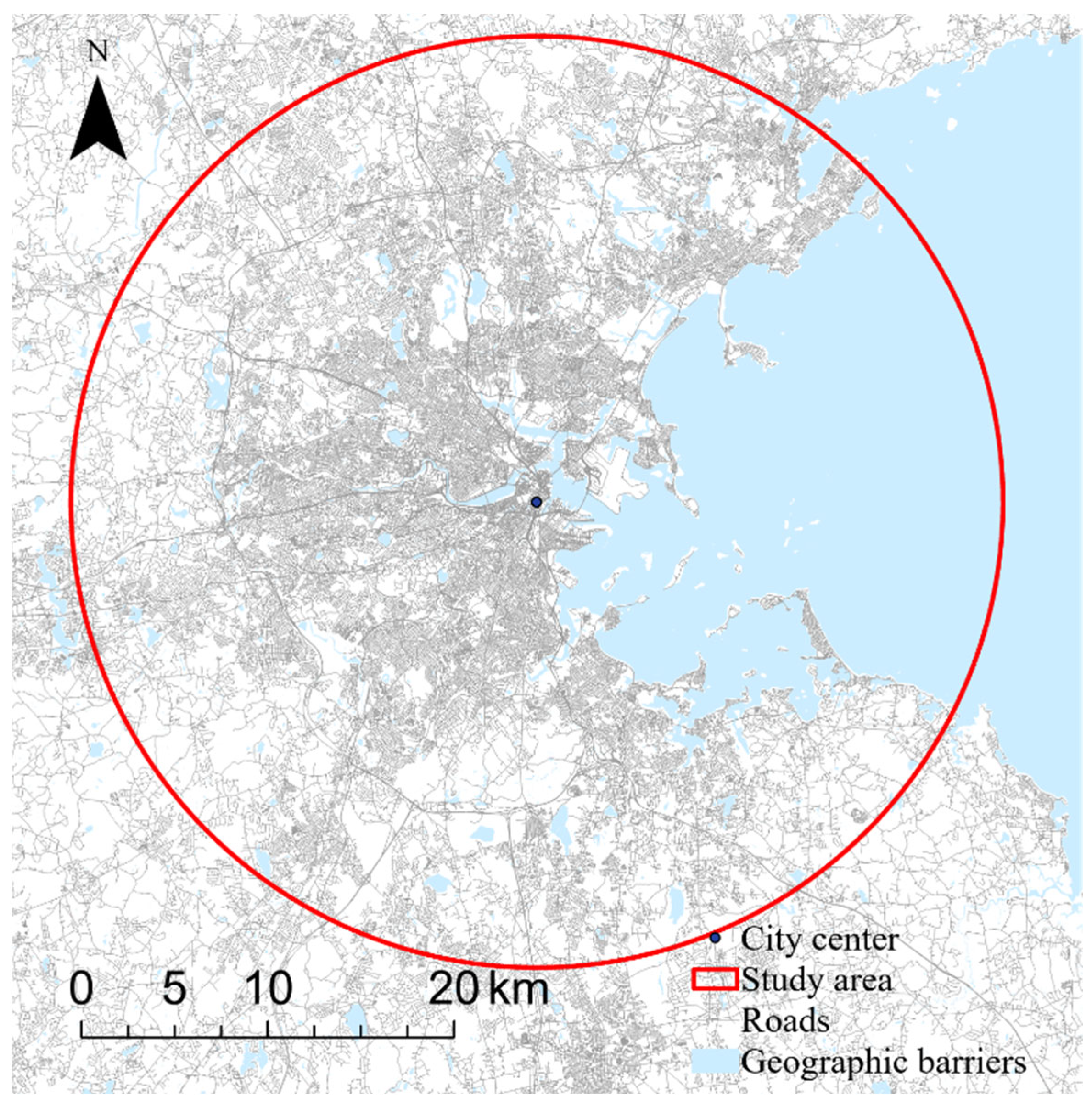
This article focuses on the city of Boston in the United States as its research area. Located on the northeastern Atlantic coast of the United States (Figure 1), Boston has coordinates of 0°01 West longitude and 52°58 North latitude. It serves as the capital and the largest city of Massachusetts and stands as the most populous city in the New England region of the northeastern United States. Bordered by the Atlantic Ocean, Boston is a quintessential port city. It encompasses a total area of 232.1 , of which land constitutes 125.4 , and bodies of water cover a substantial 106.7 . The terrain in and around Boston is predominantly flat, with the majority of the regions lying at low elevations; the highest point, Bellevue Hill, reaches only 101 m.
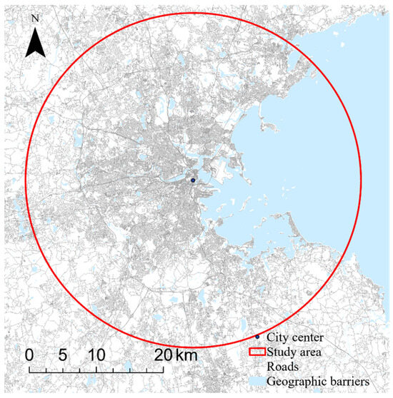
Figure 1.
The study area of Boston. The Red line is the regional boundary of the 25 km built-up area of Boston. Blue areas represent the geographic barriers (bodies of water). Grey lines denote the road networks in Boston.
Boston stands as the most populous and densely populated city in the New England region. As of 2020, the city proper had approximately 675,000 permanent residents, with the entire Greater Boston area housing around 4.5 million people [26]. Among American cities with populations exceeding 500,000, only San Francisco and Washington, D.C., have smaller land areas than Boston. Nonetheless, due to the concentration of highly developed education and financial industries in the coastal city center, a significant number of residents commute daily from the outskirts to the heart of the city. In 2019, Boston was ranked by INRIX as the most congested city in the United States and the second most congested in North America, trailing only Mexico City [27]. According to INRIX statistics, Boston commuters spend an average of 149 h annually in transit, resulting in a productivity loss averaging $2205 per commuter—figures considerably higher than the national average (99 h and $1377).
The traffic congestion in Boston can be attributed to several factors. The streets of downtown Boston, originally laid out to meet the needs of several centuries ago, consist of numerous narrow and disorganized alleys, highly unfavorable for traffic flow. Additionally, high living costs and a homogenization of employment opportunities are also recognized as pivotal factors contributing to Boston’s congestion [28]. The severe traffic issues in Boston reflect a growing challenge for numerous cities, and as a typical coastal city, exploring the relationship between its job–housing balance and geographical terrain holds significant representative value. For computational efficiency, this article has demarcated a study area encompassing a circular region centered around Boston’s Central Business District (CBD) with a radius of 25 km, essentially covering Boston’s built-up area (Figure 1).
2.2. Data Sources
2.2.1. Geographic Barriers and Road Networks
Referring to Saiz (2010) [24] for the classification of undevelopable and challenging-to-develop land, the main geographic barriers impacting the road network layout in the Boston area are identified as bodies of water and steep slopes with gradients exceeding 15 degrees. These bodies of water encompass oceans, rivers, lakes, reservoirs, and ponds. The data on the bodies of water is derived from the GlobeLand30-2010 land use dataset, released by China’s National Geomatics Center in 2014 (http://www.globallandcover.com, last accessed on 1 November 2023) [29]. GlobeLand30 is a high-resolution global land cover dataset developed by China, with versions for 2000 and 2010 released in 2014. The dataset features a 30 m spatial resolution and encompasses ten primary land cover types: cultivated land, forest land, grassland, shrubland, wetland, bodies of water, tundra, artificial surfaces, bare land, glaciers, and permanent snow. An update of this dataset was initiated by the Ministry of Natural Resources in 2017, and the GlobeLand30 2020 edition has since been completed. For the purposes of this article, only the data pertaining to bodies of water has been extracted.
The slope data is sourced from the Shuttle Radar Topography Mission (SRTM) digital elevation data, disseminated by NASA’s Land Processes Distributed Active Archive Center in 2015, featuring a spatial resolution of 1 arc-second (approximately 30 m) [30]. Using ArcGIS Pro 3.0.1 for spatial analysis and slope extraction functions, this article has extracted information on bodies of water and slopes in the Boston area with gradients over 15 degrees. The resulting distribution of geographic barriers is depicted in Figure 1. Through calculations performed in ArcGIS Pro, we have determined that the coverage of steep slopes is quite limited, accounting for less than 1% of the total geographic barriers. Therefore, we will disregard the impacts of steep slopes and focus solely on measuring the proximity of tracts to the ocean in the subsequent analysis.
Additionally, the vector road network data for Boston, also represented in Figure 1, is obtained from the U.S. Geological Survey [31]. This data, recorded in 2013, employs the WGS84 coordinate system and is part of the United States Census data, available for public use. It includes a comprehensive attribute description, featuring 35 attributes such as road names, road types, road widths, speed limits, surface materials, construction dates, among others.
2.2.2. Data on the Job–Housing Distribution of Commuters in Boston
This paper utilizes the residence and employment location data of individual commuters in Boston, sourced from the Longitudinal Employer-Household Dynamics Origin-Destination Employment Statistics (LEHD-LODES) [32]. This dataset offers annual employment distribution information for several states in the United States, spanning from 2002 to 2020, and is based on census geographic blocks divided into spatial units. The paper focuses on the spatial distribution data of employment and housing for employees in the Massachusetts area in 2020. Released on 21 March 2023, the data encompasses 2,773,263 valid records (where the number of employees in the grid is greater than 0). Each record includes the total number of commuters residing in block A and working in block B, the number by age group, the number by type of work, and the census numbers for both grids (sample data, Table 1). As this data is presented in text form, to map it onto the geographic space, the paper utilizes the spatial distribution vector data of the 2018 Boston census grid provided by the official website of the U.S. Bureau of Statistics (https://www2.census.gov/, last accessed on 1 November 2023), which includes district numbers. In ArcGIS Pro 3.0.1, the text information of the employed individuals is matched to the spatial statistical grid according to block number.

Table 1.
Structure of LEHD-LODES data.
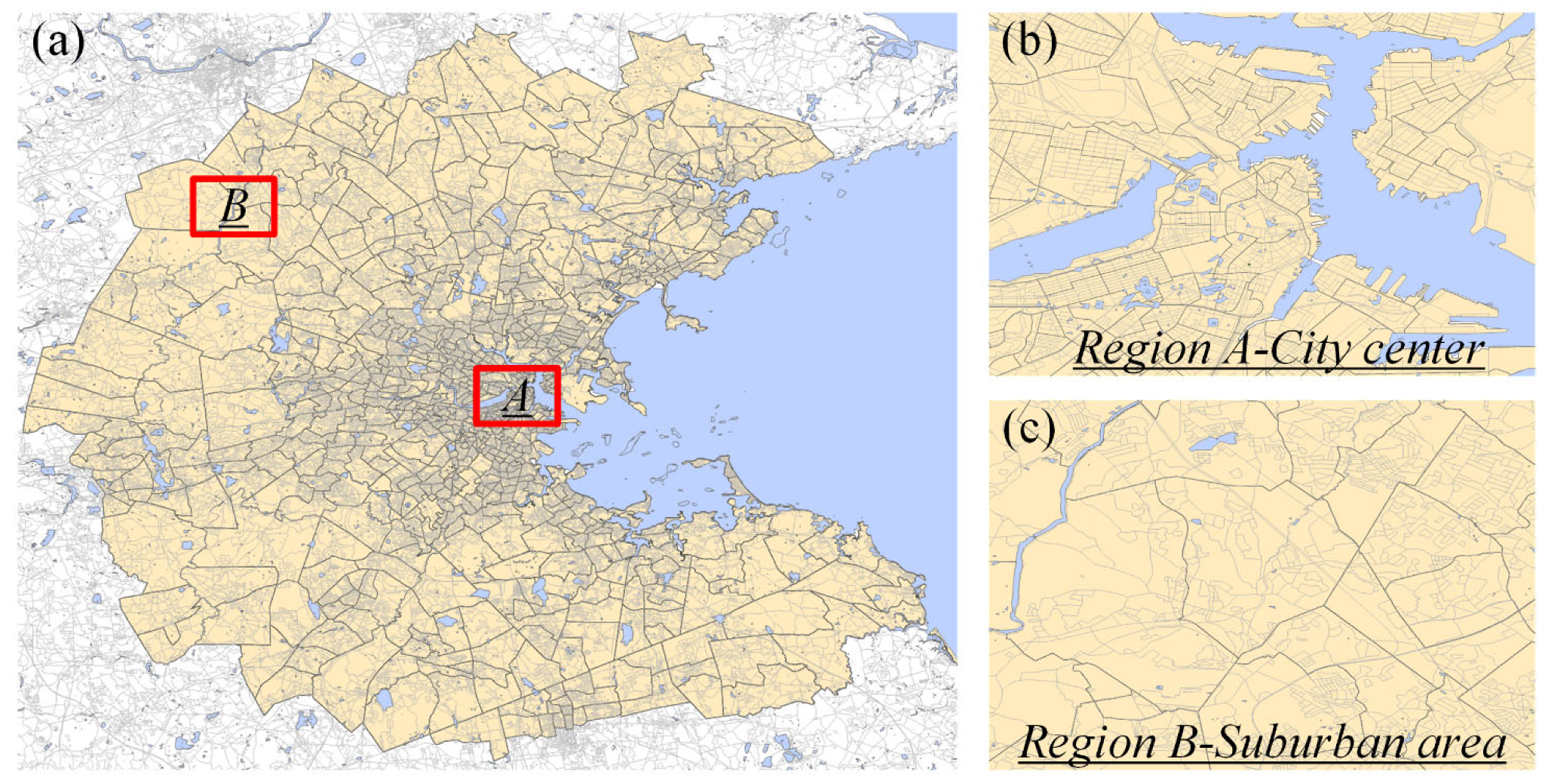
In addition to census blocks, tract data for Massachusetts was also procured from the U.S. Census Bureau’s 2020 data release (https://www.mass.gov/info-details/massgis-data-2020-us-census#tracts-, last accessed on 1 November 2023) [33]. Tracts are small, relatively permanent statistical subdivisions of a county and typically host a total population ranging between 1200 and 8000 people, with an optimum size of 4000 people. A census tract may encompass several census blocks, as depicted in Figure 2, and its boundaries remain stable over time, facilitating statistical comparisons from one census to the next. Besides spatial distribution information, the tracts dataset also comprises the basic socioeconomic attributes of the tract, such as population, number of housing units, and land area.

Figure 2.
(a) The tracts and census blocks in study area of Boston. Orange regions with black boundaries represent the tracts within 25 km of Boston’s city center and grey lines are the boundaries of census blocks. Two sample regions A and B are selected to show their details. (b) The details of a coastal region A. (c) The details of an inland region B.
3. Methods
3.1. Job–Housing Balance Indicators
Researchers have been delving into the relationship between jobs and housing for an extended period of time, introducing a plethora of indicators to evaluate the job–housing balance from various perspectives. Several metrics have been proposed to describe the job–housing balance, like the job–housing ratio (JHR), resident balance Index (RBI), and worker balance index (WBI), which assess job–housing dynamics of through the ratio of specific groups working or living within a geographical area [34,35]. There are also other measurements of the distribution of people’s job–housing choices, like the spatial mismatch index (SMI), which is mainly generated by evaluating whether specific inner-city groups (like the black population) are disproportionately disadvantaged in accessing neighborhood job opportunities [36]. The calculation is performed through a gravity-based method that assumes that job opportunities are evenly decreased from the city center to suburban regions, and places lower than the estimations are thought of as job–housing imbalance regions. Nonetheless, the application of the SMI to cities like Boston is impeded by the presence of geographical impediments and multiple discrete employment hubs, challenging the assumption of a homogeneous job distribution. Excessive commuting (EC), which corresponds to the discrepancy between the actual commute and the theoretical minimum commute, has been considered in previous studies [37]. However, these are primarily derived from travel survey data, which face limitations such as small sample sizes and low spatial-temporal resolution. This has led to the development of new indices, such as the commuting connection intensity (CCI), calculated through cell phone signaling data and traffic data. These, however, are challenging to collect and may raise privacy concerns [38]. Consequently, metrics like the job–housing ratio (JHR), residential balance index (RBI), and worker balance index (WBI) are widely utilized owing to their proven effectiveness in capturing the fundamental aspects of the job–housing balance and their relative simplicity in methodology [39,40].
(1) Job–housing ratio (JHR): The JHR is a simple metric that calculates the number of jobs available per housing unit in a specific area. This ratio reflects the balance between employment and housing capacity [35]. A JHR greater than 1 indicates a surplus of jobs (more jobs than residents), while a JHR less than 1 signifies a housing surplus. An area is considered to have achieved a job–housing balance when the JHR is approximately equal to 1.
where represents the JHR in census block and represents the number of residents that worked at block , and represents the number of residents lived within block . For the dataset in Boston, we have found that most census blocks—especially the ones near the city center, are very small and the numbers of residents working or living in the blocks is less than 3. That means that the calculation of the JHR in these blocks may lack statistical significance. Therefore, we realize that the tract-level JHR can be calculated as a potential solution, which can be generated by:
where represents the JHR index of tract t and t(n) represents the number of census blocks in tract t.
(2) Resident balance index (RBI): The RBI is an improved version of the JHR that quantifies employment opportunities close to where workers live. The index provides a very detailed view of whether the available housing stock is in line with local labor demand. The RBI calculates the ratio of individuals who both live and work in a given geographic area to the total number of residents in that area [41]. The closer the index value is to 1, the higher the resident-based job–housing balance. The formula is expressed as follows:
where denotes the RBI index in census block and denotes the number of residents living and working in census block . Considering the lack of enough records in most blocks, we then generate the tract-level RBI index:
(3) Worker balance index (WBI): The WBI is utilized to measure the balance within the workplace’s proximity to housing from the perspective of the employment centers. It focuses on the distribution of jobs across various residential areas, assessing whether there are adequate housing options near workplaces facilitating shorter commutes for different employment sectors [41]. A value approaching 1 signifies a more balanced worker-oriented job–housing relationship. The equation is outlined as follows:
where denotes the WBI index in census block . We then calculate the tract-level indicators as:
3.2. Measuring of Geographic Barriers
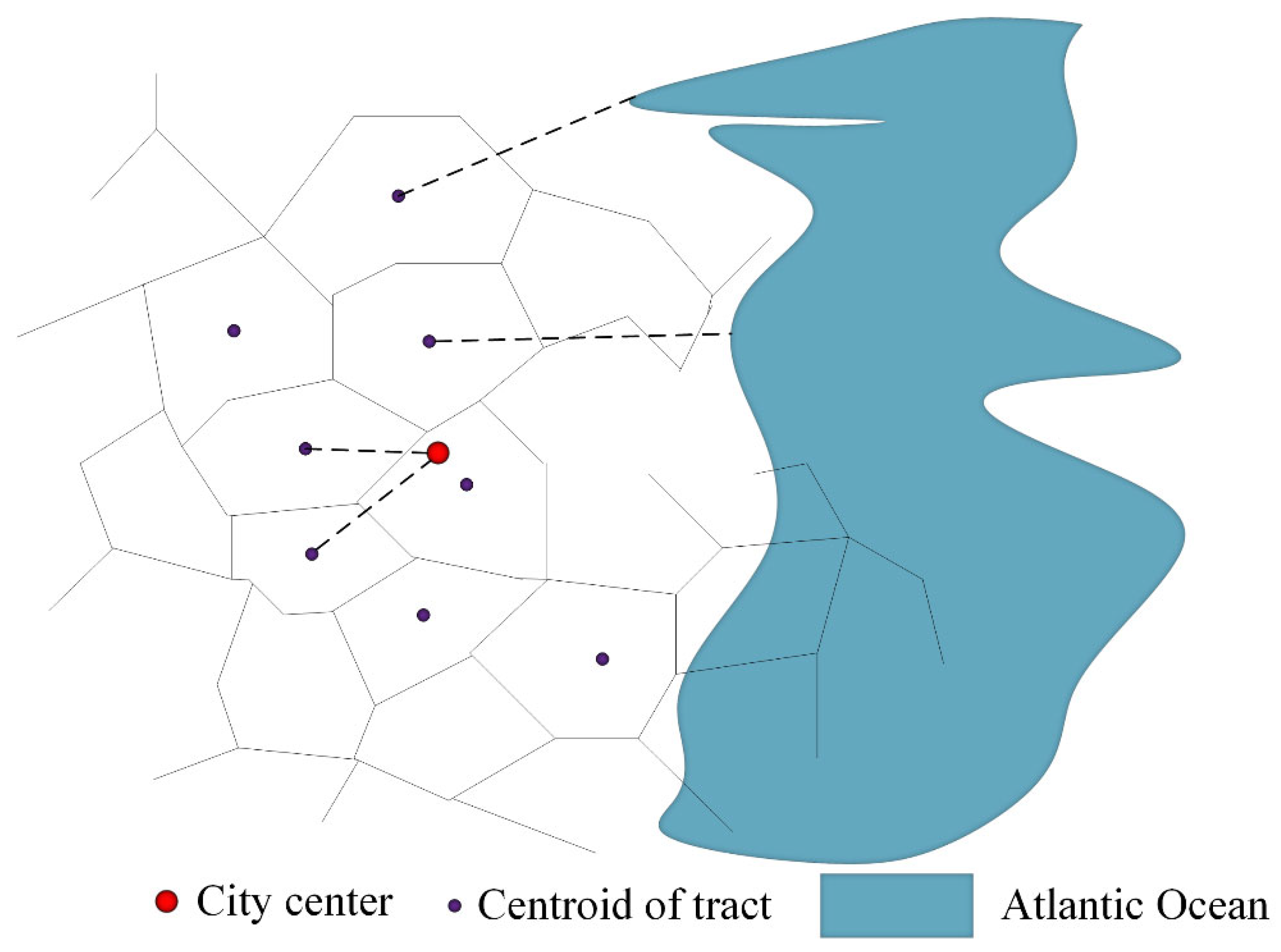
Based on our prior research, areas near large natural barriers may experience reduced commuting efficiency and congestion, particularly in proximity to these regions. The Atlantic Ocean has been identified as a primary geographic barrier contributing to traffic congestion in Boston. Consequently, we calculated the shortest straight-line distance from the centroid of each census tract to the Atlantic Ocean. This serves as a metric to measure the proximity of human residences to significant barriers, as depicted in Figure 3. This process is executed using the near module in ArcGIS Pro 3.0.2, and the shortest distance from tract t to the ocean is represented by .

Figure 3.
The calculation of the proximity of human residences to large barriers and the city center.
From Figure 2, it is evident that the city center of Boston is also situated in the coastal area of the Atlantic Ocean. Based on our prior research, we understand that city centers are also major congestion points. This implies that in Boston, the city center can have an effect similar to coastal areas—creating a unique geographical characteristic. Interestingly, regions near the central business district (CBD) may experience a combined negative effect from both the city center and geographical barriers. To differentiate the effects originating from the city center, we calculated the shortest distance from each tract t to the city center as a control variable—this is depicted in Figure 3 and represented by .
3.3. Road Network Density
Road networks are the most important infrastructure connecting residences and job centers. Therefore, we need to consider of the spatial distribution of road networks as a control and calculate the road density of each census tract:
where denotes the road segments located within tract , denotes the total land area (exclude bodies of water) of tract , and is the road density of tract .
3.4. General Ordinary Least Squares (OLS) Model
In socioeconomics, adverse factors such as high housing prices, environmental pollution, and lack of public facilities have been proven to have a direct or indirect impact on the residential and employment choices of urban residents. Our previous research [42] has verified that the existence of geographical barriers can reduce the commuting efficiency of commuters, leading to urban congestion. Moreover, geographical barriers in cities are long-term or even permanent, and cannot be improved through flexible adjustments; people have no choice but to endure the negative effects of geographical barriers for an extended period. Even if commuters are not aware that their daily commuting activities are directly or indirectly adversely affected by geographical barriers, their perception of congestion is indeed the most intuitive and profound. Therefore, whether the perception of congestion will affect the residential and job distribution of residents is the research objective of the model construction in this section. The job–housing balance indicator is used as the dependent variable of the model, geographical characterization indicators as the independent variables, and road length as the control variable to establish the following OLS (Ordinary Least Squares) model:
where Indicators represent the metrics that can be used to measure the job–housing balance in the city, including the number of employees working in the tract, the number of employees living in the tract, the JH, WBI, and RBI. is the main variable of interest, and the others are control variables describing the socioeconomic characteristics of the tract.
4. Results
4.1. Employees’ Job–Housing Spatial Distributions
Geographic barriers increase the commuting distance for commuters, thereby extending their commuting time and impacting their commuting efficiency. At the same time, the existence of geographical barriers has implications for cities whose centers are located by the sea, especially former port cities. The presence of geographical barriers directly drives a large number of affected commuters towards the city center, exacerbating congestion in the central area. This, in turn, conveys the negative impact of geographical barriers on traffic to those commuters who are not directly affected by them. The quantification of this impact is calculated based on the number and spatial distribution of commuters. However, the number and spatial distribution of commuters themselves may also be influenced by geographic barriers.
Figure 4a,b illustrates the spatial distribution of employees’ job locations and housing location choices in Boston, respectively. It is evident that a majority of employees reside in the northern and southern parts of Boston—most tracts in these two directions have a resident number exceeding 1793. However, we do not observe a similar trend of aggregation for housing choices in the city center—most tracts in the city center have fewer than 1074 residents. Examining the spatial distribution of housing choices relative to the eastern ocean, we notice that tracts closer to the ocean seem to have a greater number of housing choices compared to those farther away. This could be attributed to the appealing amenities near the ocean and the more convenient public infrastructure in the Boston coastal area—which is also proximate to the city center of Boston.
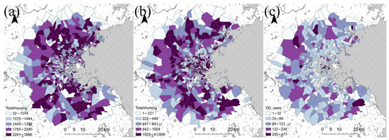
Figure 4.
The spatial distribution of employees’ job and housing locations. (a) The number of employees working at each census tract. (b) The number of employees living in each census tract. (c) The number of employees working and living in the same census tract.
Regarding the distribution of employees’ job locations, we observe an aggregating trend in the city center and in an annular area around 10 km away from the city center—the margin of the urban built-up area, with the number of jobs in these tracts exceeding 1952. Contrary to the distribution of housing choices, we do not identify a noticeable aggregation trend of jobs in regions close to the ocean, especially in several tracts located near the city center. A plausible explanation could be that the coastal regions have limited accessibility to the city’s resources, diminishing the attractiveness for companies to establish their operations there. Furthermore, challenging traffic conditions and associated higher commuting costs might also deter people from seeking employment opportunities in these locations.
Figure 4c depicts the spatial distribution of employees whose job and housing choices are situated in the same census tract—indicating an optimal job–housing balance. We observe that tracts with a high job–housing balance are primarily located on the city’s edges—far from both the city center and the ocean. This suggests that areas with better geographic conditions might achieve a superior job–housing balance. However, this pattern might also be attributed to the fact that these places are somewhat isolated from the major job centers, and residents here mainly have access to employment opportunities in their vicinity.
The distribution of employees’ job and housing location choices can impact the job–housing balance. Figure 5 displays the spatial distribution of the three indicators used to measure this balance.
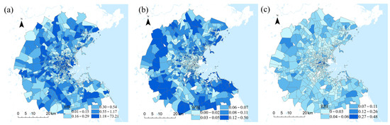
Figure 5.
The spatial distribution of job–housing balance indicators. (a) The distribution of the JHR in each census tract. (b) The distribution of the WBI in each census tract. (c) The distribution of the RBI in each census tract.
Figure 5a illustrates the distribution of the JHR in Boston, with deeper colors representing a higher ratio of jobs compared to houses. The distribution of the JHR exhibits a trend closely aligned with the distribution of the total housing choices observed in Figure 4a—both the city center and tracts in the margin (10 km annular) area of the built-up area exhibit a higher aggregation of job distributions, with their JHR ratio exceeding 1.2. Besides the city center, major job locations are distributed in the inland area, away from natural barriers. Tracts adjacent to geographic barriers often exhibit a low JHR index, indicating these areas are predominantly residential and lack job opportunities, with the exception of a few tracts located near the city center. Figure 5b presents the distribution of the WBI, offering complementary information regarding whether employees are from nearby census blocks. It is noticeable that tracts in the city center predominantly have a low WBI (<0.05), suggesting most employees working in the city center reside in other tracts. Tracts with a high WBI (>0.12) are primarily located far from the city center or near the ocean—mostly at the edge of the entire study area where fewer job opportunities are available. The higher rate of the WBI in these suburban areas indicates that employees in these regions face challenges in accessing satisfactory job opportunities in other tracts due to the considerable distance to job centers or challenging geographic conditions. Figure 5c depicts the distribution of the RBI, where tracts with a high RBI (>0.12) are predominantly located at the edge of our study area. Contrary to the trend of the WBI, tracts with a high RBI are observable close to the city center, although they are also distributed along the edge of the study area. This implies that residents of these tracts have a strong inclination (and rate) to work in those locations—in reality, individuals living in job centers are more likely to work near the city center to justify high rent prices while avoiding lengthy commutes. Additionally, these job centers tend to attract more commuters from other areas, resulting in a high RBI and a low WBI.
4.2. Spatial Distributions of Tracts’ Proximity to the Ocean
We calculated the straight-line distances from the centroid of each tract to the city center and the nearest coastline, respectively, and the results are depicted in Figure 6a,b. Furthermore, we obtained tract-level population data and the number of houses from the 2020 census, which are shown in Figure 6c,d. We observed a very similar distribution trend for population and housing units—tracts with a large population (>4709) and a high number of housing units (>1903) are primarily located at the edges of Boston, which are far from both the city center and the ocean. Most tracts in the city center have lower populations and fewer housing units, indicating that the majority of jobs in these areas are occupied by commuters from the suburban regions of Boston.
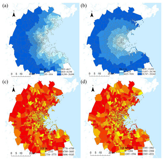
Figure 6.
(a) The spatial distribution of tracts’ proximity to the ocean. (b) The spatial distribution of tracts’ proximity to city center. (c) The spatial distribution of tracts’ census population in 2020. (d) The spatial distribution of tracts’ housing units in 2020.
4.3. Relationship between the Proximity of Geographic Barriers and Job–Housing Indicators
We then evaluated the correlation between the proximity to geographic barriers and job–housing indicators, taking into account the control of socioeconomic indices. The variables initially used are detailed in Table 2, and the results of the regression are presented in Table 3, where the logarithm of some variables is employed.
Table 2.
The descriptive statistics of variables used in regression.
Table 3.
The regression results of the job–housing indices and geographic barriers.
Our regression analyzes the impact of natural barriers on the job–housing balance in Boston, with the main dependent variable being the distance of each census tract to the ocean. The primary independent variables encompass the number of employees’ housing/job locations and three job–housing indicators. The t-statistics of the coefficients on the main independent variables are presented in parentheses beneath the estimates.
Column 1 explores the impact of natural barriers on employees’ job location choices. The number of residents working in a tract exhibits an increasing trend (coefficient = 0.102, p < 0.01) with the rise in distance to the ocean. Notably, we have accounted for the significant attraction effects (coefficient = −0.734, p < 0.01) of the city center, which are reasonable given the abundance of job opportunities there. This suggests that substantial geographic barriers can negatively affect job opportunity distribution, particularly in regions proximate to the barriers. Additionally, we have controlled for census land area and road density, both of which are significantly and positively correlated with the number of jobs (coefficient = 0.777, p < 0.01 and coefficient = 0.915, p < 0.01), indicating that convenient transportation and ample flat land are attractive to companies and factories. The finding reveals the fact that as one moves inland, away from the coastal periphery, there is an apparent concentration of employment opportunities. That can be attributed to a variety of reasons. First, tracts near the ocean often command higher land values and more expensive coastal property values, e.g., New Zealand, Boston and Los Angeles [43,44,45], largely due to their desirability for residential and recreational purposes, which can price out certain types of businesses, particularly those requiring more extensive landholdings or lower operating costs. Therefore, commercial activities that provide massive of job opportunities and do not depend on marine access or the allure of coastal proximity may find economically viable grounds further inland, where real estate is more affordable and expansive. Second, coastal zones can pose infrastructural challenges [46,47]; limited space for expansion and natural barriers may impede the development of comprehensive transportation networks, making these areas less attractive to businesses heavily reliant on logistics efficiencies. Third, environmental regulations are typically more stringent in proximity to sensitive coastal ecosystems, coupled with the heightened risks associated with coastal erosion and extreme weather events [48]. These factors can encourage businesses or companies to locate further inland to mitigate regulatory complexities and physical risks. Fourth, urban development dynamics also play a role, with coastal areas often being more mature in their development cycles, leading to a scarcity of available spaces for new or expanding businesses, pushing them towards the less developed inland areas. Additionally, inland regions may have cultivated diverse economic environments not solely reliant on the marine economy, attracting a wide array of industries through incentives, infrastructural investments, and labor force development initiatives. There is also the matter of residential preferences; coastal zones, while attractive for living, are associated with a higher cost of living [49]. Businesses may thus gravitate towards locations more accessible to a workforce seeking affordable housing options, which are more readily found as one moves away from the coast.
In column 2 of the regression analysis, the focus shifts to exploring the factors that influence residential location choices in relation to natural barriers. The data points to a distinctive trend: as individuals select places to live, there is a significant tendency to choose locations closer to the ocean, indicated by a negative coefficient of −0.0457 at a p-value below 0.01. This predilection towards coastal living may be driven by several factors, which, when woven into a narrative, form a comprehensive picture of residential dynamics. The allure of the ocean is a substantial draw for many, offering both tangible and intangible amenities that inland locations may lack. The coastal proximity typically provides scenic vistas, opportunities for recreation and leisure, and a perceived higher quality of life associated with the sea’s vicinity [50]. These attributes can contribute to a greater desire for residential spaces near the ocean, despite the potential for higher living costs and environmental risks [51]. Contrastingly, the regression results suggest that residential proximity to the city center does not hold a statistically significant relationship with the choice of dwelling location, a finding that conforms to traditional urban economic theories that high-income groups tend to live farther away from the city center for cheaper land prices and larger housing and only low-income residents aggregate near the city center, suffering from a constrained living environment to save on commuting costs. The analysis also accounts for demographic and housing variables, revealing that both the census count of the population and the number of housing units share a positive and significant relationship with residential density (coefficients of 0.132 and 0.384, respectively, with corresponding p-values of less than 0.1 and 0.01). These factors are intuitive; a higher population count within a census tract typically indicates an area with more residential housing, while a greater number of housing units directly translates to a higher potential for residential occupancy.
Column 3 reveals a nuanced relationship between the job–housing ratio (JHR) and the distance from geographic features such as the ocean. A positive coefficient of 0.246 at a significant p-value suggests that areas further from the ocean tend to exhibit higher JHR values. This is particularly insightful, considering that the JHR in most tracts under study is less than 1, signifying a general shortfall in job opportunities relative to available housing. Therefore, in areas where the JHR is higher, indicating a closer alignment between jobs and housing, it could reflect a more balanced urban structure. This balance is typically more challenging to achieve due to the difficulty in creating new employment opportunities compared to the development of residential areas. Consequently, the observation that geographic barriers correlate with a higher JHR suggests that such barriers may inadvertently encourage a more even distribution of jobs and housing by influencing urban development patterns. Column 4 provides complementary evidence, showing that the worker balance index (WBI) decreases as the distance from the ocean increases, with a coefficient of −0.00762. This inverse relationship implies that tracts located further from coastal barriers are associated with a higher presence of jobs, which is consistent with the findings in Column 1, where job location choices were influenced by proximity to the ocean. The negative correlation between the distance to the city center and the WBI indicates that suburban areas, further from the central urban zone, tend to have fewer job opportunities, aligning with the broader theme of job decentralization.
In Column 5, the resident balance index (RBI) sheds light on the flip side of the equation, focusing on residential patterns. Here, the distance to the ocean exhibits a positive correlation with the RBI, whereas the distance to the city center shows a negative one. This pattern can be interpreted as indicative of a decreasing residential density as one moves away from the urban core, a trend that was also observed in Column 2. This trend may be influenced by a variety of factors, such as the search for more affordable housing, the desire for larger living spaces, and the pursuit of a different quality of life than that offered by the dense urban environment.
These findings indicate that socio-economic dynamics affect job and housing distribution in urban areas. The regression confirms that geographic features such as the ocean not only shape the physical landscape but also exert a substantial influence on where people choose to work and live. These insights are crucial for urban planners and policymakers who must consider both the physical geography and the socio-economic fabric of the city when crafting strategies for sustainable urban growth and balanced development.
5. Discussion
5.1. Key Findings and Implications
The genesis of this research was rooted in the ongoing discourse on the influences shaping urban spatial patterns, specifically in Boston. Its geographical idiosyncrasies, coupled with its myriad of urban challenges, rendered it a compelling subject for delving into the dynamics of location choices and urban living.
- (1)
- Divergence of employees’ job–housing choices
One of the most salient findings of our study is the pronounced divergence in employees’ preferences for job and housing locations. This dichotomy illuminates the complexity of decision-making processes that underpin urban residency and employment. It was observed that while individuals displayed a propensity for residing closer to the ocean, there was a concurrent inclination towards seeking employment in areas more distant from natural barriers. This revelation triggers a cascade of reflections on the intrinsic and extrinsic factors fueling such preferences. The ocean, with its scenic allure and recreational opportunities, undeniably contributes to the perceived livability and appeal of adjacent residential areas. Conversely, the inclination for working in areas devoid of geographic barriers could be a manifestation of the quest for accessibility, economic vibrancy, and career opportunities, which are often less impeded in such locales.
The magnetism of the city center as a hub for employment was another conspicuous revelation. Despite the encumbrances posed by geographic barriers, the city center remained a focal point of employment, underscoring its indispensability in the urban employment landscape. This finding dovetails with prevailing urban theories positing the centrality of urban cores in fostering economic activities and opportunities. However, this gravitational pull towards the city center for employment did not translate equivalently to residential choices. The absence of a significant correlation between housing locations and proximity to the city center sheds light on the multifarious considerations influencing residential decisions. Factors such as housing affordability, living conditions, neighborhood amenities, and socio-cultural attributes likely converge to shape these preferences, painting a nuanced tableau of residential choice dynamics.
- (2)
- Geographic barriers and other urban planning issues
The elucidation of the relationship between geographic barriers and location choices offers a prism through which to view the broader tapestry of urban development. The juxtaposition of the allure of ocean-proximate residences with the preference for barrier-free employment locales underscores the role of geography in sculpting the urban form. Geographic constraints, such as the presence of natural barriers, inherently influence land availability, infrastructural development, and accessibility. These constraints, in tandem with human interventions, shape the urban morphology and influence the spatial distribution of residential and employment opportunities. Geographic constraints significantly influence urban development, impacting land availability, infrastructure development, and accessibility. These constraints necessitate innovative urban planning solutions to achieve a balance between job opportunities and housing.
For instance, in Hong Kong, the combination of steep terrain and limited land has led to the development of some of the most densely populated residential areas in the world [52]. The government has had to invest in extensive and efficient public transportation and embrace vertical construction to maximize the use of scarce land resources. In contrast, San Francisco’s Bay Area presents a unique challenge with its significant water barriers. The construction of the Bay Bridge and the Golden Gate Bridge were monumental infrastructure projects that allowed for greater accessibility across the bay, thus influencing residential and job distribution patterns [53]. However, these barriers continue to limit expansion and contribute to some of the highest real estate prices in the United States. Venice, Italy, is another example where geography has dictated urban form. The city’s canals serve as the main transportation routes due to the impracticality of road construction in such a water-dominated environment. This unusual geography has led to a distinctive distribution of residential and commercial spaces and has required specialized forms of infrastructure development [54]. In the case of Rio de Janeiro, Brazil, the combination of coastal areas and steep hillsides has constrained urban sprawl. The city has had to navigate these barriers by constructing favelas on steep slopes and expanding into less geographically constrained areas, resulting in a complex urban landscape with marked disparities in accessibility and infrastructure [55].
The challenges faced by these cities highlight the importance of considering geographic constraints in urban planning. Infrastructure development must be creative and adapted to the local context, and urban policies need to address the unique challenges posed by natural barriers. By examining these international examples, urban planners and policymakers can gain insights into effective strategies to mitigate the impacts of geographic constraints, promoting a more equitable and balanced urban environment, which will promote the job–housing balance and sustainable urban development.
- (3)
- Socio-economic considerations
The job and housing choices of Boston residents are closely related to geographical barriers and are also influenced by various socio-economic factors. To a certain extent, the existence of geographical barriers further amplifies its impact by affecting socio-economic factors such as housing affordability, employment opportunities, quality of life, and accessibility. The results of the previous regression analysis indicate that Boston residents prefer to live closer to the ocean, and the distribution of residents is negatively correlated with the distance from the ocean. This trend may reflect the high value placed on the amenities and quality of life associated with living near the water—a sentiment that is echoed in many coastal cities. In Boston, this is evident in the high demand for housing in areas like the Seaport District and along the East Boston Shore [56,57]. Of course, considering Boston’s historical development and zoning patterns, Boston has an extensive coastline and is frequently affected by typhoons [58]. Therefore, while the housing prices in a small number of coastal communities are high, in general, the cost of housing in most coastal areas is not significantly higher than in inland areas, which is also an important reason why most residents can afford housing by the seaside. Regarding the employment locations of Boston residents, there is a significant relationship between employment distribution and distance from the city center, indicating that most economic activities are still concentrated in the urban core of Boston, rather than by the seaside. This, of course, is related to the limited land supply and policy restrictions on coastal development, which determine that residents often face long commutes [59].
The greater Boston area’s investment in transportation infrastructure, such as the MBTA subway and commuter rail systems, attempts to mitigate some of the accessibility challenges posed by geography [60].The relationship between geographic barriers and location choices in Boston is a delicate balance of trade-offs—between the scenic allure and the higher cost of waterfront living, between the centrality of employment and the affordability of housing, and between the desire for quality of life and the realities of accessibility. As Boston continues to evolve, urban planners must carefully consider these factors to cultivate an environment where equitable access to housing, employment, and quality living can be more than just an aspiration.
5.2. Limitations and Future Work
While our study shed light on many aspects, it did have some limitations. One major limitation was the data we used. We used data from census tracts and measured straight-line distances, which meant we might have missed smaller, more detailed variations and influences on daily choices. This showed us how complex people’s movements and preferences can be and emphasized the need for more detailed data. Also, our study focused only on Boston, so we have to be careful about applying our findings to other cities with different characteristics and histories. Boston is unique, and other cities might be very different. Another limitation was that our study looked at only one point in time, using data from the 2020 census. Cities are always changing, influenced by many different factors like economics, society, demographics, and politics. This means that we need to use data from different times to fully understand how cities develop and how people’s location choices change. We also did not include some socioeconomic factors in our study, like individual income and education levels. Leaving out these factors might have limited how well we could understand the relationships between job and housing locations in the city.
Moreover, this study employs straightforward indices such as the job–housing ratio (JHR), residential building index (RBI), and workers per building index (WBI). While these indices offer valuable insights into the job and housing dynamics of urban environments, they may not capture the full complexity and nuances of such relationships. The JHR, for instance, while providing a snapshot of job availability relative to housing, does not account for the quality or type of employment, the match between jobs and local residents’ skills, or the commuting patterns that might affect job accessibility. Similarly, the RBI and WBI provide a measure of residential density and job concentration but overlook factors like the diversity of housing stock, the affordability spectrum, and the nature of the jobs considered. A more sophisticated set of indices or a multi-faceted analytical framework could yield a richer and more detailed understanding of the interplay between jobs and housing.
As for the city selection, the study’s focus on Boston brings about inherent limitations when considering the broader applicability of the findings. Boston’s unique geographic, historical, and socio-economic context may not be representative of other urban areas, especially those with different development patterns, economic bases, or demographic compositions. For example, replicating this analysis in New York City might yield different insights due to New York’s distinct urban layout, its diverse economy, and its different policy approaches to housing and employment. Additionally, factors such as public transit systems, the presence of natural barriers, and regional economic trends could significantly influence the job–housing relationship in ways not accounted for in this Boston-centric analysis. As such, caution should be exercised when attempting to apply the findings of this study to different urban settings without considering local variations and context-specific dynamics.
Looking forward, there are many possibilities for future research. One promising idea is to study a variety of cities, each with its unique features. Comparing different cities can give us better insights into common and unique urban patterns, making our findings more widely applicable. Longitudinal studies, or studies over time, could also help us understand how cities and individual choices change. Including more socioeconomic and behavioral factors in future studies could give us a fuller picture of why people choose to live and work where they do in cities. Adding qualitative research methods, like interviews, surveys, and focus groups, to our quantitative analyses would also give us a fuller view of city life. Talking to city residents could help us understand their experiences, views, and hopes, adding depth to our insights. Future research should also look at turning findings into practical recommendations. Working closely with urban planners, policymakers, and community stakeholders could help find innovative solutions to the challenges and opportunities we identified. This teamwork could help make cities more fair, sustainable, and livable. Exploring how technology affects city patterns is another exciting area for future research. Studying how new technologies like autonomous vehicles and smart city initiatives change cities could give us valuable insights into future city life and development. We also need to consider the effects of climate change on city patterns. Understanding how strategies to deal with climate change affect location choices and city development is important for creating sustainable and resilient cities. Finally, looking into urban design and quality of life can give us a full view of city living. Studying how design principles, architectural innovations, and community initiatives affect city residents’ quality of life can help create vibrant, inclusive, and sustainable city communities.
6. Conclusions
Job–housing imbalance is a growing threat for the sustainable development of our society [61,62]. The achievement of a job–housing balance is a multifaceted challenge, traditionally addressed through the lens of socio-economic factors such as race, income, and infrastructure inequality. However, a growing body of research suggests that urban structure and inefficient land use could be underlying contributors to job–housing imbalances. Yet, few have considered geographic barriers as a fundamental factor. By analyzing the spatial location data for over 3 million Boston residents, our study investigates the extent to which natural barriers influence job–housing choices. Our main contributions are as follows:
First, through statistical analysis at a grid scale, we have uncovered that people’s choices of residential location tend to favor areas close to the eastern coastal part of Boston or inland regions about 10 km away. These areas either boast attractive landscapes or offer affordable land prices, yet both are quite distant from the city center. Our findings can be instrumental for urban planners in comprehending residential location preferences on a macro level, especially in coastal cities. This insight aids in better developing transportation infrastructure and urban facilities planning in coastal regions. Consequently, it enhances service provision to residents and improves the operational efficiency of those areas.
Second, we built three indexes (JHR, WBI, and RBI) to quantify the tract-level job–housing balance in Boston and use regressions to explore their correlation with geographic barriers as well as socioeconomic issues. Our findings revealed that tracts in the margin area of the built-up zone manifest a higher concentration of job distributions, evidenced by a JHR ratio exceeding 1.2, indicating a job-rich environment. Conversely, tracts near geographic barriers and in the city center predominantly exhibit lower job–housing and work balance indices, signifying a discrepancy in residential and employment locations. The finding not only confirms the influence of geographic barriers on the job–housing balance but also provides a quantifiable measure of this impact within the context of Boston’s urban framework.
This study serves as an initial exploration and confirmation of the significant influence that geographical barriers exert on the job–housing distribution among residents. It provides a mechanistic perspective that aids in unraveling the potential reasons behind prevalent issues such as traffic congestion and the uneven distribution of housing supply prices, particularly in coastal cities. By shedding light on these intricacies, the research offers valuable insights that can guide policymakers in formulating and refining regional transportation and housing supply strategies. Moreover, it presents a framework for the development of measures aimed at enhancing employment opportunities at a macro level, with a specific emphasis on the unique challenges and dynamics present in coastal cities. The implications of the findings are substantial, extending the understanding of urban planning necessities and providing a foundation for more equitable and efficient urban development. The insights drawn from this research are instrumental in addressing both current urban challenges and anticipating future needs, thereby contributing to the overall betterment of urban living conditions, especially in geographically constrained environments.
Author Contributions
Conceptualization, L.W. and X.L.; methodology, X.L.; software, W.L.; writing—original draft preparation, L.W. and X.L.; project administration, L.W. All authors have read and agreed to the published version of the manuscript.
Funding
This research was funded by National Natural Science Foundation of China, grant number 42301493.
Institutional Review Board Statement
Not applicable.
Informed Consent Statement
Not applicable.
Data Availability Statement
All the data sources used in this study are public available and their links have been provided.
Acknowledgments
We want to thank Dongxiao Niu for her kind help during the data analysis for this paper.
Conflicts of Interest
The authors declare no conflict of interest.
References
- Jing, Y.; Hu, Y.; Niedzielski, M.A. Neighborhood divides: Where you live matters for commuting and its efficiency. Cities 2023, 132, 104091. [Google Scholar]
- Deng, Y.; Zhao, P. Quantifying residential self-selection effects on commuting mode choice: A natural experiment. Transp. Res. Part D Transp. Environ. 2022, 104, 103197. [Google Scholar]
- Islam, M.R.; Saphores, J.-D.M. An LA story: The impact of housing costs on commuting. J. Transp. Geogr. 2022, 98, 103266. [Google Scholar]
- Huang, Y.; Du, Q.; Li, Y.; Li, J.; Huang, N. Effects of Metro Transit on the Job–Housing Balance in Xi’an, China. J. Urban Plan. Dev. 2022, 148, 04021068. [Google Scholar]
- Ren, F.; Zhang, J.; Yang, X. Study on the Effect of Job Accessibility and Residential Location on Housing Occupancy Rate: A Case Study of Xiamen, China. Land 2023, 12, 912. [Google Scholar]
- Bautista-Hernández, D.A. Jobs-Housing Imbalances, Urban Segregation, and Intra-metropolitan Commute Flows in Mexico City. J. Plan. Educ. Res. 2022. [Google Scholar] [CrossRef]
- Afrin, T.; Yodo, N. A survey of road traffic congestion measures towards a sustainable and resilient transportation system. Sustainability 2020, 12, 4660. [Google Scholar]
- China Academy of Urban Planning, Urban-Rural Development. National Major Cities Commuting Time Consumption Monitoring Report; Urban Transport Infrastructure Monitoring and Management Laboratory, Ministry of Housing and Urban-Rural Development: Beijing, China, 2020. [Google Scholar]
- Liu, J.; Ettema, D.; Helbich, M. Systematic review of the association between commuting, subjective wellbeing and mental health. Travel Behav. Soc. 2022, 28, 59–74. [Google Scholar]
- Ding, C.; Liu, T.; Cao, X.; Tian, L. Illustrating nonlinear effects of built environment attributes on housing renters’ transit commuting. Transp. Res. Part D Transp. Environ. 2022, 112, 103503. [Google Scholar]
- Peña, J.; Luis, A.; Arellana, J. Which dots to connect? Employment centers and commuting inequalities in Bogotá. J. Transp. Land Use 2022, 15, 17–34. [Google Scholar]
- Luo, Z.; Wang, Y.; Lv, Z.; He, T.; Zhao, J.; Wang, Y.; Gao, F.; Zhang, Z.; Liu, H. Impacts of vehicle emission on air quality and human health in China. Sci. Total Environ. 2022, 813, 152655. [Google Scholar] [PubMed]
- Deng, F.; Lv, Z.; Qi, L.; Wang, X.; Shi, M.; Liu, H. A big data approach to improving the vehicle emission inventory in China. Nat. Commun. 2020, 11, 2801. [Google Scholar] [PubMed]
- Long, Y.; Thill, J.-C. Combining smart card data and household travel survey to analyze jobs–housing relationships in Beijing. Comput. Environ. Urban Syst. 2015, 53, 19–35. [Google Scholar]
- Zhu, P.; Ho, S.N.; Jiang, Y.; Tan, X. Built environment, commuting behaviour and job accessibility in a rail-based dense urban context. Transp. Res. Part D Transp. Environ. 2020, 87, 102438. [Google Scholar]
- Alonso, W. Location and Land Use: Toward a General Theory of Land Rent; Harvard University Press: Cambridge, MA, USA, 1964. [Google Scholar]
- Muth, R.F. Cities and Housing: The Spatial Pattern of Urban Residential Land Use; The University of Chicago Press: Chicago, IL, USA, 1969. [Google Scholar]
- Mills, E.S. Studies in the Structure of the Urban Economy. Econ. J. 1972, 83, 289–291. [Google Scholar]
- Lin, X.; Zhong, J.; Ren, T.; Zhu, G.J.C. Spatial-temporal effects of urban housing prices on job location choice of college graduates: Evidence from urban China. Cities 2022, 126, 103690. [Google Scholar]
- Yao, Z.; Kim, C. Analyzing the multiscale patterns of jobs-housing balance and employment self-containment by different income groups using LEHD data: A case study in Cincinnati metropolitan area. Comput. Environ. Urban Syst. 2022, 96, 101851. [Google Scholar]
- Harari, M. Cities in bad shape: Urban geometry in India. Am. Econ. Rev. 2020, 110, 2377–2421. [Google Scholar] [CrossRef]
- Duque, J.C.; Lozano-Gracia, N.; Patino, J.E.; Restrepo, P.; Velasquez, W.A. Spatiotemporal dynamics of urban growth in Latin American cities: An analysis using nighttime light imagery. Landsc. Urban Plan. 2019, 191, 103640. [Google Scholar]
- Angel, S.; Franco, S.A.; Liu, Y.; Blei, A.M. The shape compactness of urban footprints. Prog. Plan. 2018, 139, 100429. [Google Scholar]
- Saiz, A. The geographic determinants of housing supply. Q. J. Econ. 2010, 125, 1253–1296. [Google Scholar] [CrossRef]
- Ahlfeldt, G.M.; McMillen, D.P. Tall buildings and land values: Height and construction cost elasticities in Chicago, 1870–2010. Rev. Econ. Stat. 2018, 100, 861–875. [Google Scholar] [CrossRef]
- Tsirikos, A.I.; Adam, R.; Sutters, K.; Fernandes, M.; García-Martínez, S. Effectiveness of the Boston Brace in the Treatment of Paediatric Scoliosis: A Longitudinal Study from 2010–2020 in a National Spinal Centre. Healthcare 2023, 11, 1491. [Google Scholar] [CrossRef] [PubMed]
- Basu, R.; Sevtsuk, A. How do street attributes affect willingness-to-walk? City-wide pedestrian route choice analysis using big data from Boston and San Francisco. Transp. Res. Part A Policy Pract. 2022, 163, 1–19. [Google Scholar] [CrossRef]
- Ei Leen, M.W.; Jafry, N.H.A.; Salleh, N.M.; Hwang, H.; Jalil, N.A. Mitigating Traffic Congestion in Smart and Sustainable Cities Using Machine Learning: A Review. In Proceedings of the International Conference on Computational Science and Its Applications, Athens, Greece, 3–6 July 2023; pp. 321–331. [Google Scholar]
- Chen, J.; Chen, J. GlobeLand30: Operational global land cover mapping and big-data analysis. Sci. China Earth Sci. 2018, 61, 1533–1534. [Google Scholar] [CrossRef]
- Farr, T.G.; Kobrick, M. Shuttle Radar Topography Mission produces a wealth of data. Eos Trans. Am. Geophys. Union 2000, 81, 583–585. [Google Scholar] [CrossRef]
- Liu, H.; Li, H.; Rodgers, M.O.; Guensler, R. Development of road grade data using the United States geological survey digital elevation model. Transp. Res. Part C Emerg. Technol. 2018, 92, 243–257. [Google Scholar] [CrossRef]
- Schleith, D.; Horner, M.W. Commuting, job clusters, and travel burdens: Analysis of spatially and socioeconomically disaggregated longitudinal employer–household dynamics data. Transp. Res. Rec. 2014, 2452, 19–27. [Google Scholar] [CrossRef]
- Logan, J.R.; Xu, Z.; Stults, B.J. Interpolating US decennial census tract data from as early as 1970 to 2010: A longitudinal tract database. Prof. Geogr. 2014, 66, 412–420. [Google Scholar] [CrossRef]
- Sultana, S. Job/housing imbalance and commuting time in the Atlanta metropolitan area: Exploration of causes of longer commuting time. Urban Geogr. 2002, 23, 728–749. [Google Scholar] [CrossRef]
- Ta, N.; Chai, Y.; Zhang, Y.; Sun, D. Understanding job-housing relationship and commuting pattern in Chinese cities: Past, present and future. Transp. Res. Part D Transp. Environ. 2017, 52, 562–573. [Google Scholar] [CrossRef]
- Liu, C.Y.; Painter, G. Immigrant settlement and employment suburbanisation in the US: Is there a spatial mismatch? Urban Stud. 2012, 49, 979–1002. [Google Scholar] [CrossRef]
- Ma, K.R.; Banister, D. Excess commuting: A critical review. Transp. Rev. 2006, 26, 749–767. [Google Scholar] [CrossRef]
- Wang, J.; Zhou, C.; Rong, J.; Liu, S.; Wang, Y. Community-detection-based spatial range identification for assessing bilateral jobs-housing balance: The case of Beijing. Sustain. Cities Soc. 2022, 87, 104179. [Google Scholar] [CrossRef]
- Wang, X.; Hua, Z.; Li, J. Cross-UNet: Dual-branch infrared and visible image fusion framework based on cross-convolution and attention mechanism. Vis. Comput. 2023, 39, 4801–4818. [Google Scholar] [CrossRef]
- Wang, H.; Zeng, W.; Cao, R. Simulation of the urban jobs–housing location selection and spatial relationship using a multi-agent approach. ISPRS Int. J. Geo-Inf. 2021, 10, 16. [Google Scholar] [CrossRef]
- Li, Z.; Zhao, P.; Yu, L.; Hai, X.; Feng, Y. The changes in job-housing balance during the COVID-19 period in China. Cities 2023, 137, 104313. [Google Scholar] [CrossRef]
- Saiz, A.; Wang, L. Physical geography and traffic delays: Evidence from a major coastal city. Environ. Plan. B Urban Anal. City Sci. 2023, 50, 218–243. [Google Scholar] [CrossRef]
- Collins, D.; Kearns, R. Uninterrupted views: Real-estate advertising and changing perspectives on coastal property in New Zealand. Environ. Plan. A Econ. Space 2008, 40, 2914–2932. [Google Scholar] [CrossRef]
- Severen, C.; Plantinga, A. Land-use regulations, property values, and rents: Decomposing the effects of the California Coastal Act. J. Urban Econ. 2018, 107, 65–78. [Google Scholar] [CrossRef]
- Jin, D.; Hoagland, P.; Au, D.K.; Qiu, J. Shoreline change, seawalls, and coastal property values. Ocean Coast. Manag. 2015, 114, 185–193. [Google Scholar] [CrossRef]
- Azevedo de Almeida, B.; Mostafavi, A. Resilience of infrastructure systems to sea-level rise in coastal areas: Impacts, adaptation measures, and implementation challenges. Sustainability 2016, 8, 1115. [Google Scholar] [CrossRef]
- Su, X.; Belvedere, P.; Tosco, T.; Prigiobbe, V. Studying the effect of sea level rise on nuisance flooding due to groundwater in a coastal urban area with aging infrastructure. Urban Clim. 2022, 43, 101164. [Google Scholar] [CrossRef]
- Zheng, H.; Zhang, L.; Zhao, X. How does environmental regulation moderate the relationship between foreign direct investment and marine green economy efficiency: An empirical evidence from China’s coastal areas. Ocean Coast. Manag. 2022, 219, 106077. [Google Scholar] [CrossRef]
- Ayoola, A.B.; Oladapo, A.R.; Ojo, B.; Oyetunji, A.K. Modelling coastal externalities effects on residential housing values. Int. J. Hous. Mark. Anal. 2022. [Google Scholar] [CrossRef]
- Free, C.M.; Smith, J.G.; Lopazanski, C.J.; Brun, J.; Francis, T.B.; Eurich, J.G.; Claudet, J.; Dugan, J.E.; Gill, D.A.; Hamilton, S.L.J.P.; et al. If you build it, they will come: Coastal amenities facilitate human engagement in marine protected areas. People Nat. 2023, 5, 1592–1609. [Google Scholar] [CrossRef]
- Haque, M.O.; Aman, J.; Mohammad, F. Construction sustainability of container-modular-housing in coastal regions towards resilient community. Built Environ. Proj. Asset Manag. 2022, 12, 467–485. [Google Scholar] [CrossRef]
- Chen, S.; Bao, Z.; Lou, V. Assessing the impact of the built environment on healthy aging: A gender-oriented Hong Kong study. Environ. Impact Assess. Rev. 2022, 95, 106812. [Google Scholar] [CrossRef]
- Bollapragada, R.; Kakar, V.; Goodwin, J.; Fremier, A. Adoption of FasTrak on San Francisco Bay Area Bridges: Impact of Operations Research Models in Relieving Congestion. INFORMS J. Appl. Anal. 2023, 53, 97–110. [Google Scholar] [CrossRef]
- Saldarini, A.; Colombo, C.G.; Longo, M.; Brenna, M.; Miraftabzadeh, S.M.; Yaici, W. Water Transport Decarbonization: Preliminary Case Study in Venice. In Proceedings of the 2023 IEEE International Conference on Electrical Systems for Aircraft, Railway, Ship Propulsion and Road Vehicles & International Transportation Electrification Conference (ESARS-ITEC), Venice, Italy, 29–31 March 2023; pp. 1–4. [Google Scholar]
- Costa, L.L.; Bulhões, E.M.R.; Caetano, J.P.A.; Arueira, V.F.; de Almeida, D.T.; Vieira, T.B.; Cardoso, L.J.T.; Zalmon, I. Do costal erosion and urban development threat loggerhead sea turtle nesting? Implications for sandy beach management. Front. Mar. Sci. 2023, 10, 1242903. [Google Scholar] [CrossRef]
- Simlai, P. Estimation of variance of housing prices using spatial conditional heteroskedasticity (SARCH) model with an application to Boston housing price data. Q. Rev. Econ. Financ. 2014, 54, 17–30. [Google Scholar] [CrossRef]
- Glaeser, E.L.; Schuetz, J.; Ward, B. Regulation and the Rise of Housing Prices in Greater Boston; Harvard University: Cambridge, MA, USA, 2006. [Google Scholar]
- Brugge, D.; Rice, P.W.; Terry, P.; Howard, L.; Best, J. Housing conditions and respiratory health in a Boston public housing community. New Solut. A J. Environ. Occup. Health Policy 2001, 11, 149–164. [Google Scholar] [CrossRef] [PubMed]
- Giuliano, G.; Hou, Y.; Kang, S.; Shin, E.-J. Accessibility, Location, and Employment Center Growth; METRANS Transportation Center (Calif.): Los Angeles, CA, USA, 2015. [Google Scholar]
- Horan, C. Neoliberalizing infrastructure: Financing public transportation in Greater Boston. J. Urban Aff. 2023, 1–20. [Google Scholar] [CrossRef]
- Guo, S.; Pei, T.; Xie, S.; Song, C.; Chen, J.; Liu, Y.; Shu, H.; Wang, X.; Yin, L. Fractal dimension of job-housing flows: A comparison between Beijing and Shenzhen. Cities 2021, 112, 103120. [Google Scholar] [CrossRef]
- Lin, S.; Wang, N.H.C.; Van Ameijde, J. The Sub-Urbanisation of New Towns: The Influence of Job-Housing Imbalance on Low-Income Groups’ Job Opportunities in Tin Shui Wai, Hong Kong. Evol. Sch. 2022. [Google Scholar] [CrossRef]


Disclaimer/Publisher’s Note: The statements, opinions and data contained in all publications are solely those of the individual author(s) and contributor(s) and not of MDPI and/or the editor(s). MDPI and/or the editor(s) disclaim responsibility for any injury to people or property resulting from any ideas, methods, instructions or products referred to in the content. |
© 2023 by the authors. Licensee MDPI, Basel, Switzerland. This article is an open access article distributed under the terms and conditions of the Creative Commons Attribution (CC BY) license (https://creativecommons.org/licenses/by/4.0/).