Energy-Saving Speed Planning for Electric Vehicles Based on RHRL in Car following Scenarios

Abstract

Eco-driving is a driving vehicle strategy aimed at minimizing energy consumption; that is, it is a method to improve vehicle efficiency by optimizing driving behavior without making any hardware changes, especially for autonomous vehicles. To enhance energy efficiency across various driving scenarios, including road slopes, car following scenarios, and traffic signal interactions, this research introduces an energy-conserving speed planning approach for self-driving electric vehicles employing reinforcement learning. This strategy leverages vehicle-to-vehicle (V2V) and vehicle-to-infrastructure (V2I) communication to acquire real-time data regarding traffic signal timing, leading vehicle speeds, and other pertinent driving conditions. In the framework of rolling horizon reinforcement learning (RHRL), predictions are made in each window using a rolling time domain approach. In the evaluation stage, Q-learning is used to obtain the optimal evaluation value, so that the vehicle can reach a reasonable speed. In conclusion, the algorithm’s efficacy is confirmed through vehicle simulation, with the results demonstrating that reinforcement learning adeptly modulates vehicle speed to minimize energy consumption, all while taking into account factors like road grade and maintaining a secure following distance from the preceding vehicle. Compared with the results of traditional adaptive cruise control (ACC), the algorithm can save 11.66% and 30.67% of energy under two working conditions.

1. Introduction

At present, electric vehicles (EVs) stand as one of the most promising technologies in the realm of transportation for enhancing energy efficiency and mitigating CO₂ [1]. Additionally, in reducing carbon dioxide emissions, vehicle design and aerodynamic resistance play a crucial role, as improving the aerodynamic performance of vehicles can significantly reduce energy consumption [2]. However, limited driving range and battery energy storage hinder the development of electric vehicles. In terms of energy replenishment, it takes more time to recharge electric vehicles than it does to refuel traditional fuel vehicles. Furthermore, in most places, there are far fewer charging stations for electric vehicles than there are gas stations. The energy consumption of electric vehicles depends on many aspects, such as battery charge level, the reasonable allocation of battery capacity, electric vehicle performance, road conditions, driving strategy, driving style, etc. [3,4,5]. Hence, how to effectively utilize the limited energy storage of electric vehicles is a very important issue.

At present, the real-time communication of connected and autonomous vehicles (CAVs) provides a proactive view of traffic conditions through V2V [6], V2I [7], and advanced sensors. Among them, vehicle-to-vehicle (V2V) refers to communication between vehicles, allowing them to exchange data and information directly. Meanwhile, vehicle-to-infrastructure (V2I) involves communication between vehicles and roadside infrastructure, such as traffic lights or road sensors, enabling vehicles to interact with the surrounding environment for improved traffic management and safety. These predictions have opened up unprecedented opportunities for electric vehicles to improve safety, mobility, and energy efficiency. Speaking of energy efficiency in the realm of eco-driving, various strategies and algorithms have been developed to minimize energy consumption in vehicle operations. The eco-driving strategy, as proposed by Qiu in reference [8], has demonstrated the potential to achieve energy savings ranging from 4% to 10% across various operational scenarios. Nevertheless, the eco-driving algorithm introduced in reference [9], which utilizes signal phasing and timing (SPaT) data along with geographic intersection description (GID) information and forecasts the state of the vehicle ahead, offers a seamless and energy-efficient trajectory, resulting in a notable 4.0% reduction in energy consumption. Moreover, an energy-efficient speed planning approach [10] rooted in dynamic programming has been devised, involving real-time interaction with traffic signals when passing through signalized intersections. Schwickart [11] introduced dynamic speed planning aimed at generating an optimal speed profile for a specific time span, taking into account initial conditions and electric traction status to minimize energy consumption. However, while the literature mentioned above includes extensive research on vehicle energy efficiency, it often overlooks the intricate relationship between vehicle dynamics and energy usage, as well as uncertainties associated with real-time fluctuations in driving scenarios.

To address this challenge, numerous energy consumption control algorithms have been developed. For instance, there is a control algorithm rooted in the principles of acceleration and coasting [12]. Moreover, a range of optimal control theories have been applied, encompassing dynamic programming (DP), Pontryagin’s minimum principle (PMP), and model predictive control (MPC), among other methodologies. The DP algorithm, which hinges on the Bellman equation [13], has been extensively explored with different DP-based methods [14,15], such as forward-looking DP [16], to seek optimal solutions. Nevertheless, this method is computationally demanding and struggles with real-time adaptability in dynamic driving environments. The PMP-based approach has been utilized in various investigations [17,18], where it converts the optimal control problem into a constrained optimization task. Significantly, an alternative algorithm for managing kinetic energy and fuel conversion [19], influenced by the equivalent consumption minimization strategy, has been put forth. This algorithm integrates control principles akin to those found in the PMP. In parallel, MPC-based methods have received attention, improving vehicle dynamics modeling and offering hierarchical control strategies. Furthermore, it considers the exceptional accuracy and resilience of speed prediction. He [20] studied the MPC-based method and established an enhanced vehicle longitudinal dynamics model considering powertrain response performance as the prediction model. In another study, Wang [21] proposed a MPC-based hierarchical eco-driving control strategy for HEVs in hybrid driving scenarios. Hosseinzadeh [22] et al. applied MPC to integrate traffic sign data and other vehicle-specific information. This allowed for the dynamic adjustment of both the safe distance and the ideal speed. Consequently, this approach not only bolstered safety measures but also resulted in reduced fuel consumption across a defined distance. Meanwhile, Iman [23] studied the impact of automation and cooperative systems on mixed traffic including conventional vehicles and adaptive cruise control (ACC) vehicles. Furthermore, ACC is an advanced driver assistance system that automatically controls a vehicle’s cruise speed based on the speed and distance of the vehicle in front to maintain a safe following distance, enhancing driving comfort and safety.

Nevertheless, the aforementioned model-based control techniques necessitate the creation of accurate dynamic system and driving environment models, with the model’s precision significantly impacting controller performance. The vehicle’s operating environment, in particular, is characterized by its intricacy and variability, rendering accurate predictions challenging. Consequently, applying these control methodologies to vehicle controllers represents a formidable task. As an alternative, machine learning (ML) approaches are garnering substantial attention. Compared to traditional control strategies, ML methods offer the distinct advantage of not mandating precise physical models of vehicle power systems or driving conditions. Instead, they facilitate the extraction or learning of control strategies in a data-driven fashion. Within the realm of ML techniques, reinforcement learning (RL) strategies have emerged as a focal point of research in eco-driving control.

RL functions by furnishing agents with a system of rewards and penalties as necessary. When confronted with a problem, the aim of RL is to improve an agent’s actions by means of a trial-and-error process, driven by a variety of exploration strategies stemming from the agent’s interactions within its ever-changing environment. The ultimate aim is for the agent to determine and execute the optimal action that yields the highest reward. RL has found applications in numerous optimal control problems, particularly in the domain of energy management for electric vehicles, such as RL with forward-looking concepts [24], model-based RL for hybrid electric vehicles [25], or RL for energy management with fuel cell vehicles [26]. In reference [27], Lee introduces a model-based RL approach designed for achieving eco-driving control in pure electric vehicles. This technique involves a clear separation between the approximated model of vehicle energy consumption and the model representing the driving environment. A study compares autonomous vehicles with conventional cruise control vehicles under constant speed driving conditions. In the work by Shi [28], a RL-driven strategy for eco-driving at crossroads is introduced, incorporating V2I communication. The study assesses the practicality of this approach and the results indicate that a RL-based energy management system (EMS) can foster eco-conscious driving behaviors, diminish emissions, and enhance traffic efficiency. In [29], the problem of vehicle speed planning at signalized intersections is studied using the RL method, and using the deep Q-learning method at unsignalized intersections. Bai [30] used DRL to develop advanced driving behavior decisions for connected vehicles implemented in heterogeneous traffic scenarios. The algorithm exhibits strong performance in terms of its learning efficiency and robustness. Additionally, it demonstrates impressive generalization capabilities, especially when confronted with diverse traffic scenarios.

However, while the aforementioned studies utilized RL, none of them addressed the simultaneous consideration of the road gradient and safe distance to the preceding vehicle. References [31,32] took into account the distance to the preceding vehicle but assumed a road gradient of 0. Conversely, reference [33] primarily concentrated on eco-driving strategies pertaining to specific intersection scenarios, rather than addressing a broader spectrum of driving situations. Within the realm of eco-driving, the incline of the road plays a critical role in shaping vehicle energy consumption, particularly when considering energy consumption during uphill climbs, downhill coasting, or regenerative braking for energy conservation. Consequently, it becomes imperative to incorporate road slope information into vehicle speed planning optimization. Moreover, given the inherent presence of other vehicles on the road, it is imperative to consider the constraint of maintaining a safe distance from the vehicle ahead.

This research introduces an eco-driving strategy tailored for car following situations, taking into account road gradients and traffic signal conditions. This study makes the following noteworthy contributions:

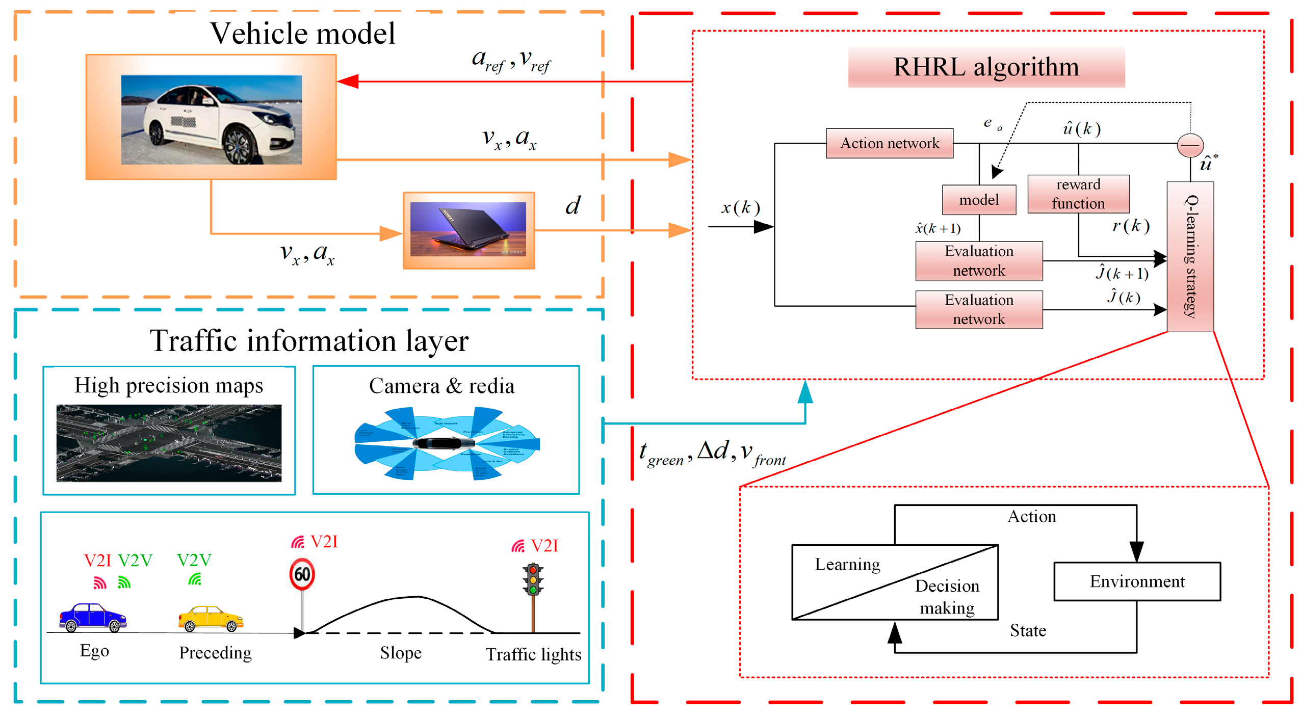
• A RHRL algorithm is put forward to enhance the eco-driving strategy for EVs. This algorithm takes into account both the road gradient and the car following scenario at signalized intersections. More precisely, it begins by acquiring driving conditions, including the timing data of road signals and the speed data of the leading vehicle, through V2I and V2V communication.
• Within the RHRL framework, it leverages a rolling time domain approach to make predictions within each time window. In the evaluation stage, Q-learning is used to obtain the optimal evaluation value, so that the vehicle can reach a reasonable speed.
• Iterations using Transformer networks in rolling optimization.
• The effectiveness of the algorithm is verified based on the vehicle simulation results, and the energy saving performance of the car following scenario is compared with that under the ACC method.

A structure diagram of this article is shown in Figure 1. The chapters are distributed as follows. In Section 2, the vehicle dynamics model and the battery model are introduced. In Section 3, a RHRL-based eco-driving strategy considering car following scenarios is proposed. In Section 4, simulations and comparisons are performed. Finally, conclusions and future work are given in Section 5.

2. Model Building

In this study, the electric vehicle is driven by four permanent magnet synchronous motors, and the battery is a lithium-ion battery. To reduce complexity, the model is mainly simplified by ignoring some small effects, such as mechanical and power converter losses.

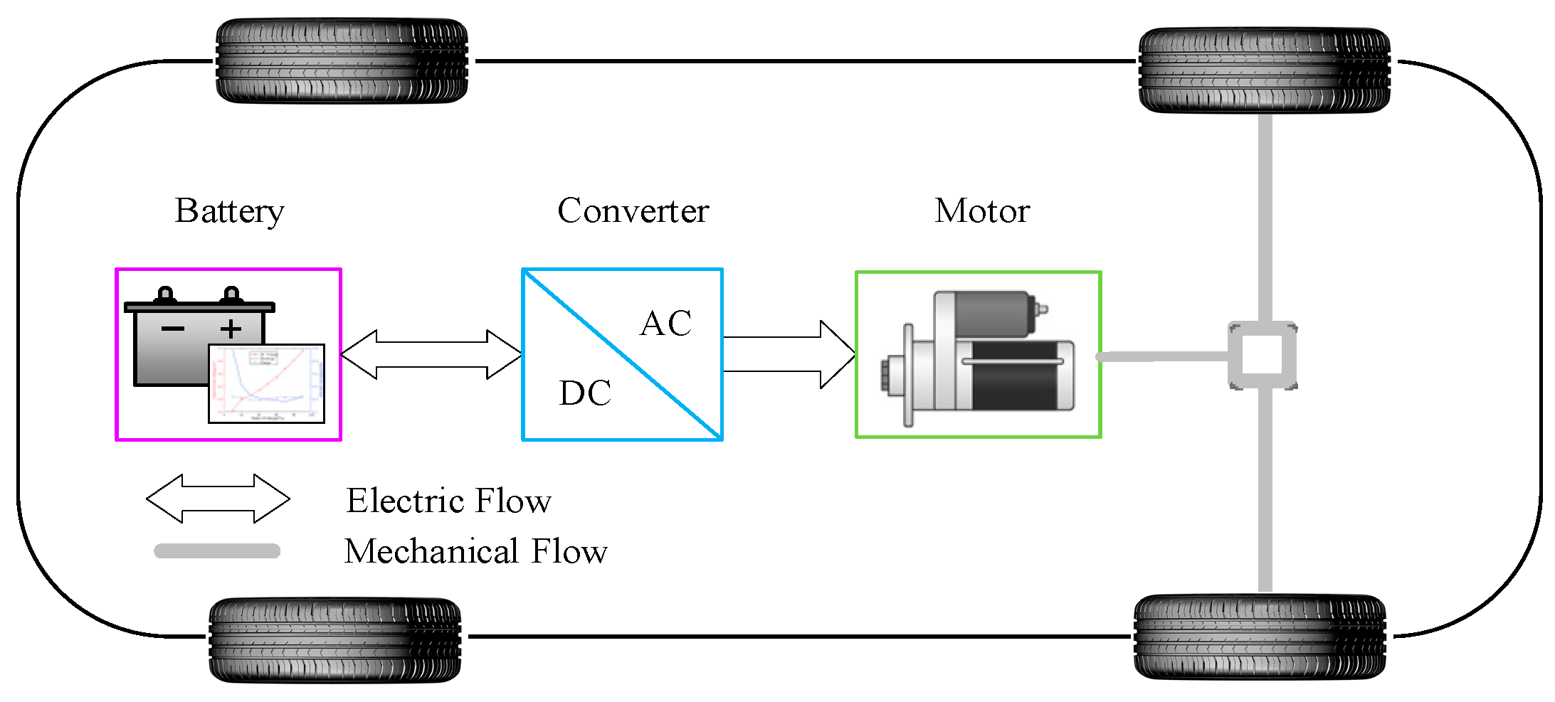
2.1. Vehicle Dynamics Model

Within the eco-driving speed planning model, only the longitudinal kinematics of the vehicle are taken into account. The model is outlined as follows:

$$\dot{d}(t)=v(t)$$

(1)

$$\dot{v}(t)=a=\frac{T_{whl}/R-F_r}{M_{eq}}$$

(2)

where d is the distance traveled by the vehicle, v is the vehicle speed, a is the acceleration of the vehicle, T_whl is the torque of the vehicle, R is the tire radius, F_r represents the vehicle resistance, and M_eq is the total mass of the vehicle, including the inertia of the rotating parts in the power system. While the vehicle is in motion, the motor’s output torque is transmitted to the wheels via the transmission system, resulting in the generation of a driving force that balances the resistance encountered during the drive.

$$F_r=mgf\cos \alpha +mg\sin \alpha +\frac{1}{2}\rho A{c}_d{v}^2$$

(3)

Among the symbols, m represents the mass of the vehicle, g represents the acceleration of gravity, f represents the rolling resistance coefficient, ρ is the air density, A is the windward area, c_d is the air resistance coefficient, and α is the road slope. As shown in Figure 2, the powertrain of the vehicle consists of the battery system as the primary energy source, providing energy to the motor through an inverter.

2.2. Battery Model

In the energy management system (EMS) of RHRL, the battery not only provides peak energy and recovers braking energy, but also plays a vital role in overall vehicle efficiency. Generally, battery models can be divided into electrochemical models, data models, and equivalent circuit models. The equivalent circuit model has the advantages of simple structure, fewer parameters, and high computational efficiency in describing and modeling the external characteristics of the battery, and is more suitable for the simulation of battery energy optimization problems. In this study, the Rint model [34] is selected as the equivalent circuit model. Finally, with this model, the output power of the battery is as follows:

$$P_b=U_{ocb}{I}_b-R_b{I}_b^2$$

(4)

where U_ocb is the open circuit voltage, I_b is the battery current, and R_b is the internal resistance. The numerical model characteristics of the battery are shown in Figure 3a. As shown in Figure 3b, this is the battery model used in the experiments. The battery current, as determined by the equivalent circuit, depends on the battery’s output power, internal resistance, and open circuit voltage, and can be expressed as follows:

$$I_b=\frac{U_{ocb}-\sqrt{U_{ocb}^2-4R_b{P}_b}}{2R_b}$$

(5)

The battery state of charge (SOC) is discretized, and its transfer equation is as follows:

$$SOC(k+1)=SOC(k)-\frac{I_b(k)}{Q_m}\mathsf{\Delta }t$$

(6)

where Q_m is the battery capacity.

3. Eco-Driving Optimization Functions and Constraints

To realize the optimization of the eco-driving speed trajectory, RHRL mainly realizes vehicle speed optimization. The goal is to reduce the frequency of acceleration and braking operations by using V2I and V2V to obtain information such as signal lights, speed limits, and vehicles in front, to determine a reasonable vehicle speed and ensure the lowest possible energy consumption. Combining Equations (1) and (2), this study employs a discrete-time kinematic differential equation to model and analyze the motion of the vehicle, providing insights into its dynamic behavior over time. The equation is as follows:

$$d(k+1)=d(k)+v(k)\Delta T+0.5a(k)\Delta T^2$$

(7)

$$v(k+1)=v(k)+a(k)\Delta T$$

(8)

In Equations (7) and (8), k is the current moment, and ΔT is the sampling period. In this study, the acceleration within each sampling period is regarded as a constant (ΔT = 0.01 s). It can be expressed as an optimal control problem in ecological driving. Setting the state vector as x$={\left[x_1{, x}_2\right]}^T{=[d, v]}^T$, input$u=\left[a\right]$. The power system can be described as follows:

$$x(k+1)=x(k)+f(x(k),u(k))$$

(9)

3.1. Eco-Driving Objective Function

Considering the system design goal, the energy consumption in the prediction time domain is selected as the objective function, and at the same time, other penalty items are added based on the energy consumption to ensure the driving comfort and dynamic performance of the vehicle. Given the reference speed, v_ref, and the terminal speed constraint, v_f, the objective function is constructed to optimize the ecological driving speed, and the following cost function is proposed [35]:

$$\min J={\displaystyle \sum _{k=0}^{N-1}(C(x(k),u(k)),\Delta T)}+\mathrm{\Gamma }[x(k+N)]$$

(10)

Among the symbols, ${\displaystyle \sum }_{k=0}^{N-1}(C\left(x\left(k\right),u\left(k\right)\right), \Delta T)$ is the overall energy consumption, and N represents the prediction step size, which is calculated via the overall prediction time, T_s, and the sampling period, ΔT. Its expression is as follows:

$$N=\frac{T_s}{\Delta T}$$

(11)

In this paper, T_s is calculated from the time series of upcoming traffic lights obtained via V2I, and the predicted time length decreases as the running time increases. In Equation (10), the expression for C is as follows:

$$C(x,u,k)={\omega }_{1}P(x,u,k)+{\omega }_2{\Vert u(k)-u(k-1)\Vert }^2$$

(12)

where ω₁ and ω₂ are the weight coefficients. P(x) represents the energy consumption function, and $u\left(k\right){-u(k-1)}^2$ is the amplitude constraint of the system control input, which is used to prevent excessive acceleration and reduced comfort. $\mathsf{\Gamma }\left[x\right(k+N\left)\right]$ indicates the system status:

$$\mathrm{\Gamma }[x(k+N)]={\omega }_3{(v(k_f)-v_f)}^2+{\omega }_4{(d(k_f)-d_f)}^2$$

(13)

where ω₃ and ω₄ are the weight coefficients. v_f is the terminal speed, and d_f is the terminal distance, which is determined by the position of the road signal light ahead. The terminal travel time, k_f, is fixed and is affected by the signal light sequence.

The light sequences from V2I will be used as constraints for the optimization problem. At the intersection, combined with the status of the signal lights at the two intersections ahead and the remaining time, the vehicle speed is planned and limited, and the number of starts and stops of the vehicle is reduced while ensuring compliance with traffic rules, to achieve the purpose of reducing energy consumption. There are generally three situations where a vehicle receives a traffic light: acceleration, cruise, and deceleration. The initial speed of the cruising speed is v_d, and the terminal speed, v_f, is determined by whether the vehicle passes the traffic light or not. To save energy, the vehicle must accelerate or decelerate at the appropriate time if it cannot pass the intersection at the current speed. Signal phase and timing (SPaT) and the distance, Δd, between the vehicle and the signal light are necessary to select the appropriate driving mode.

If the vehicle cannot pass by immediately accelerating to the maximum speed, ${\min \{v}_{\max }{,v}_{\mathrm{front}}\}$, when the light is green, it will decelerate in advance and wait for the next green light cycle, so the terminal speed in this case is v_f = 0. Another situation is when the vehicle maintains a constant speed or when it accelerates through the intersection while the vehicle maintains a constant speed or is subject to terminal speed constraints, v_f = v_d. The upper boundary of the vehicle speed is $v_{\max }=\min \{\left(1+\epsilon \right)v_d{, v}_{\lim }\}$, where $v_{\lim }$ is the vehicle speed limit, and ε is a parameter that represents the allowable range of the vehicle speed, which can be obtained through learning algorithms and statistical analysis. In the second scenario, assuming that the vehicle in front is driving at a speed of v_front, if the distance to the vehicle in front meets the speed and acceleration requirements, the host vehicle will still pass or stop according to the remaining green phase of the upcoming traffic light. While the vehicle’s speed tolerance is affected by the vehicle in front, the host vehicle must obey intelligent driving model (IDM) rules [36]. The speed limit is $v_{\max }{=\max \{v}_{\mathrm{front}}, \left(1+\epsilon \right)v_d{, v}_{\lim }\}$. By comparing $v_{\max }{ \times t}_{\mathrm{green}}$ and Δd, you can decide whether to pass the intersection or not, and obtain the terminal speed. Since the termination time of vehicles traveling on a fixed road section is determined via the timing of traffic lights, the terminal time of the optimal control problem, t_f, is fixed, and the prediction time domain decreases with time. Assuming that the current moment is t, and the forecast time domain is T, then the forecast time domain at each moment is ${T=t}_f-t$, and the constraints need to be satisfied as follows:

$$\{\begin{array}{l}\mathrm{\Gamma }[x(k+N)]={\omega }_3{(v(k_f)-v_f)}^2+{\omega }_4{(d(k_f)-d_f)}^2\hfill \\ v_0=v_d,d_0=0\hfill \\ v_{\min }(k)\le v(k)\le v_{\max }(k)\hfill \\ a_{\min }(k)\le a(k)\le a_{\max }(k)\hfill \end{array}$$

(14)

In Equation (14), $v_{\min }{\left(k\right), v}_{\max }\left(k\right)$ is the vehicle speed limit obtained through traffic information, and $a_{\min }{\left(k\right), a}_{\max }\left(k\right)$ is the acceleration limit.

3.2. Speed Dynamic Programming Based on Transformer and RL

To obtain the optimal vehicle speed of an economical cruise in real time, that is, to solve the optimal solution of the speed in the speed planning problem, this paper proposes a rolling time domain dynamic programming method to solve the speed of the cruise control system. In each discretized prediction domain, the Transformer network is used to solve the optimal control sequence, the control quantity of the optimized sequence is applied to the system for rolling, and the next optimization is started. The algorithm structure is shown in Figure 4.

3.2.1. Action Network

In this paper, the Transformer model is adopted as the action network to approximate the control input u(k). The Transformer model utilizes a multi-head self-attention mechanism to extract relevant information at different positions within time series data. The multi-head self-attention mechanism divides the model into multiple self-attention modules, forming multiple subspaces to allow the model to focus on different aspects of information, and integrating information from various aspects helps the network capture richer features [37]. Therefore, the action network in this paper adopts the Transformer network structure of time series prediction, as shown in Figure 4. The input state variable, ${x=[x}_1{, x}_2{]}^T{=[d, v]}^T$, is the distance and speed of the vehicle, which are obtained through network action taking into account safety, comfort, and car following conditions, and providing corrections for speed planning through Q-learning.

Regarding the Transformer model structure, as shown in Figure 5, the Transformer encoder operates on the input state vector, converting it into an embedding vector before passing it on to the encoder blocks. The Transformer decoder operates on previously generated corresponding outputs and the encoded input sequence from the middle branch to output the next state in the output sequence. The sequence of previous output states (used as inputs to the decoder) is obtained by shifting the output vectors one position to the right and adding a start-of-vector token at the beginning. This shifting method prevents the model from merely copying the decoder input to the output.

First comes position encoding (position embedding). Since the Transformer does not use the structure of RNN, but uses global information, it cannot use the sequence information of the input data, and this part of the information is very important for time series prediction. To solve this problem, the Transformer uses position embedding to save the relative or absolute position of the input vector in the sequence. Position encoding mainly uses sine and cosine functions, namely [37] the following:

$$\{\begin{array}{c}PE(pos,2i)=\sin (\frac{pos}{{10000}^{2i/d_{\mathrm{model}}}})\\ PE(pos,2i+1)=\cos (\frac{pos}{{10000}^{2i/d_{\mathrm{model}}}})\end{array}$$

(15)

Among the symbols, pos is the current position; 2i is the even dimension; 2i+1 is the odd dimension; d_model is the number of input features; when the subscript is 2i, PE indicates the position information obtained when the dimension is even; and when the subscript is 2i + 1, PE indicates the position obtained when the dimension is odd information.

Secondly, for the encoder, the Transformer follows the commonly used encoder–decoder structure. To prevent network degradation and accelerate convergence, the encoder also uses residual connections and layer normalization. When relying on time series learning, the Transformer’s scaled dot product attention function [37] is as follows:

$$Attention(Q,K,V)=soft\max (\frac{Q{K}^T}{\sqrt{d_k}})V$$

(16)

where $Q\in K^{n\times d}, K\in K^{N\times d}, v\in K^{N\times d}$ are the query, key, and value matrices, respectively, N is the sequence length, and d is the hidden dimension in each attention. $soft\max$ is used for the activation function of multi-classification; to prevent the inner product from being too large, it needs to be divided by $\sqrt{d_k}$.

The multi-head self-attention mechanism contains multiple self-attention layers, and is essentially a linear transformation after splicing the results of multiple attention calculations so that the model can obtain different feature information [37].

$$M(Q,K,V)=Concat(h_1,h_2,\cdots ,h_{h^{\prime }})W^o$$

(17)

$$h_i=Attention(Q{W}_i{}^Q,K{W}_i{}^K,V{W}_i{}^V)$$

(18)

Among the symbols, h′ represents the total number for attention, W^o represents the weight matrix, and the Concat function is the concatenation operation of the vector. ${\mathrm{W}}_{\mathrm{i}}^Q,$ ${\mathrm{W}}_{\mathrm{i}}^K$, and ${\mathrm{W}}_{\mathrm{i}}^v$ represent the weight matrix corresponding to the input of the i-th head.

Furthermore, the function of the feed-forward network (FFN) is to prevent the degradation of the model output. It is a two-layer fully connected layer. The activation function of the first layer is the Relu function, and the activation function of the second layer is not used. The corresponding formula is as follows:

$$F_{FFN}(x)=\max (0,x{W}_1+b_1)W_2+b_2$$

(19)

Among the symbols, W₁ and W₂ are the weight matrices; b₁ and b₂ are the bias items; x is the input of the fully fed network.

Finally, the features obtained by the encoder in the prediction layer are added to with global average pooling before the fully connected layer to reduce the parameters that need to be optimized in the fully connected layer to alleviate the overfitting problem.

3.2.2. Reward Network

In RHRL, the return function can be strengthened or weakened as a training indicator. This study takes the energy consumption performance of the target vehicle on roads with traffic signal constraints as a return function indicator, and establishes a one-step reward function based on the ecological driving performance indicator of Equation (10):

$$\begin{array}{cc}\hfill r_i(x(k),u(k),k)& ={\beta }_1{C}_i(x(k),u(k),k)+\hfill \\ & {\beta }_2{\Vert u_i(k)-u(k-1)\Vert }^2+{\beta }_3{\Vert v_i(k)-v_f\Vert }^2+\hfill \\ & {\beta }_4{f}_i(\Delta d-d_{safe})\hfill \end{array}$$

(20)

where ${\beta }_1$, ${\beta }_2$, ${\beta }_3$, and ${\beta }_4$ are the weight coefficients, and d_safe is the safe distance between vehicles. At this time, combining Equations (10)–(12), the system’s return function is as follows:

$$J\left(x(k),k\right)=\mathrm{\Gamma }\left[x(k+N)\right]+{\displaystyle \sum _{j=k}^{k+N-1}{\gamma }^{j-k}r(x(j),u(j))}$$

(21)

3.2.3. Evaluation Network

The evaluation network selection of error-based error functions is first given the general Q-Learning optimal control strategy, ${\mathsf{\pi }}^{*}\left(x_k\right)=\mathrm{argmin}\left(Q^{*}\left(x_k,u\right)\right)$, and optimal cost, ${\mathrm{J}}^{*}\left(x_k\right)=\min \left(Q^{*}\left(x_k,u\right)\right)$. Among them, the Q factor represents the action value function [38], which is represented by the following:

$$Q^{\ast }(x_k,u_k)=g(x_k,u_k)+\gamma J^{\ast }(x_{k+1})$$

(22)

To determine the value of the Q function, the action value function is updated as follows:

$$Q\left(x_k,u_k\right)\leftarrow Q\left(x_k,u_k\right)+\alpha (g_k+\gamma \min Q\left(x_{k+1},u\right)-Q\left(x_k,u_k\right))$$

(23)

In Q-Learning, the control input is determined by the Q function. In Equation (23), the Q function’s value can be adjusted through interactions between the vehicle’s status and the evaluation function. By monitoring and utilizing the instantaneous pricing and subsequent changes in the vehicle’s state variables, the Q function value r_k can be updated. This update incorporates both estimated rewards and an estimated follow-up evaluation function, Ĵ_k+1. For the relative distance between different speeds and vehicles, when the time step is k, for $k=1,2,3,\cdots ,N$, all the allowable movements to iterate the Q function update, as shown below:

$$Q\leftarrow (1-\alpha )Q\left(J(k),u_k^l\right)+\alpha \left({\widehat{g}}_k+\gamma \min Q\left(\widehat{J}(k+1),u_k\right)\right).$$

(24)

In this article, α takes the value 0.05, and γ takes the value 0.9995.

The algorithm pseudo-code is given in Algorithm 1. The characteristics of this algorithm are that some of the fields that can be modeled in the algorithm’s configuration can improve the efficiency of the RL algorithm. In the part that is difficult to model, the model-free RL is used to make full use of the advantages of the modeless method to reasonably find the optimal energy consumption.

Algorithm 1 RHRL algorithm.

Obtain the timing information of road signal lights and the speed information of the preceding vehicle through V2I and V2V, and then set the length of the prediction layer and the sampling time interval. The initial state of the vehicle represents the initial values of parameters such as action network, criticism network, and learning rate. The maximum number of iterations is na. 1: for $t_j=T_c,2T_c,\cdots$ do 2:  for $k=t_j,t_j+1,\cdots ,t_j+N-1$ do 3:    Apply the action network to get $\widehat{u}(k)$. 4:    The next state estimate $\widehat{x}(k+1)$ is obtained from the model and the state values. $r(k)$ comes from the reward function. 5:    Input $\widehat{x}(k)$ and $\widehat{x}(k+1)$ into the evaluation network to get $\widehat{J}(k)$ and $\widehat{J}(k+1)$. 6:    Observe and update Q. 7:  for $k=1,2,\cdots ,n_a$ do 8:    $Q\leftarrow (1-\alpha )Q\left(J(k),u_k^l\right)+\alpha \left({\widehat{g}}_k+\gamma \min Q\left(\widehat{J}(k+1),u_k\right)\right).$ (Equation (24)) 9:    end for 10:   Update action network and evaluation network. 11:  end for 12: end for

4. Simulation Results

As shown in Figure 6, the experimental platform includes a driving simulator, the running control algorithm dSPACE, a real-time vehicle model running the target machine and console, and a SCANeR traffic scene host. The driver manipulates the accelerator pedal in the driving simulator to simulate the driving of the vehicle in front. The traffic scene module sends the speed signal to the target machine according to the real-time traffic information and vehicle state, and obtains the new position and state changes of the vehicle at the same time. Finally, it is sent to the traffic scene host and the speed planning module. The speed planning module is implemented and developed based on MATLAB code, and simulated on the workstation. The CPU of the workstation is Intel (R) Core (TM) [email protected] GHz, and the RAM is 64.0 GB. The relevant parameters of the vehicle are listed in

Table 1. Vehicle parameters.

Symbol	Value [Unit]	Symbol	Value [Unit]
m	1800 [kg]	A	2.06 [m2]
μ	0.75	$\rho$	1.18 [kg/m3]
R	0.322 [m]	g	9.8 [m/s2]
CD	0.36	f	0.0074

, and the relevant limitations of the powertrain are listed in

Table 2. The values of minimum and maximum powertrain system parameters.

Parameter	Value [Unit]	Parameter	Value [Unit]
Torque_motor_min	10 [Nm]	Torque_motor_max	800 [Nm]
N_motor_min	50 [rpm]	N_motor_max	1350 [rpm]
PW_batt_min	−339 [kW]	PW_batt_max	339 [kW]
SOC_min	4.8%	SOC_max	99.2%

. We determine how discretized the variables are by considering the performance of the algorithm and the amount of computation required to perform discretization.

In SCANeR, the simulated scene is based on the section information on urban roads and the time series of traffic lights. There are two experimental road sections about 1.2 km long, with 10 and 14 intersections. The adopted control algorithm (RHRL) and the rule-based ACC algorithm (ACC) are tested using hardware-in-the-loop (HIL), and the sampling period is ΔT = 0.01 s. The driving route is shown in Figure 7a. The slope of the two driving routes is different as shown in Figure 7b, and the maximum height difference is about 60 m. In the car-following scene, the vehicle in front simulated in the V2V information travels at the speed shown in Figure 7c, the acceleration of the vehicle in front is shown in Figure 7d, and the initial vehicle distance is 50 m. The signal light information in the V2I information is shown in

Table 3. Road 1 traffic light position.

Intersection	Position (m)	Intersection	Position (m)
1	107	6	4776
2	1067	7	5485
3	2624	8	6129
4	3292	9	8296
5	3978	10	9891

and

Table 4. Road 2 traffic light position.

Intersection	Position (m)	Intersection	Position (m)
1	1624	8	6763
2	2657	9	7730
3	2857	10	8173
4	3041	11	8806
5	3601	12	9173
6	3894	13	9491
7	5201	14	10,440

.

In the simulation, for each driving route, the maximum number of iterations per RHRL time domain is set at $n_{\max }=50$. The learning rates for both the action network and the critic network are systematically decreased following the steps detailed in Algorithm 1. As the learning process advances, it becomes evident that the cost (accumulated for each driving route) rapidly diminishes, and efficient learning is realized. Figure 8 shows the speed planning results of the vehicle, and Figure 9 shows the scene results of following a car through a signal light. Under the influence of the maximum speed limit, the vehicle in Figure 9a learns the speed change of the vehicle ahead and decelerates reasonably in advance, while in Figure 9b, the vehicle accelerates reasonably after waiting for traffic lights, and decelerates reasonably before the front vehicle decelerates again.

The SOC comparison of ACC and RHRL for the two road conditions is shown in Figure 10. In Figure 10a, RHRL is accompanied by energy recovery under a reasonable braking system, which can effectively distribute battery power. Under RHRL, the SOC drops from 99.2% to 97.156%. At this time, the SOC is consumed from 99.2% to 97.156% under the ACC control strategy and then to 96.886%, saving about 11.66%. In Figure 10b, since the vehicle did not meet the signal lights at the beginning of the start, the energy-saving effects of RHRL and ACC are not much different in the case of simple car following, but the RHRL is prominent after passing through several signal lights. After 1200 s, the SOC of RHRL dropped from 99.2% to 97.316%, while that of ACC dropped from 99.2% to 96.482%. The former saved about 30.67% compared with the latter. For the two working conditions, the working efficiency of the motor is shown in Figure 11.

5. Conclusions and Future Work

This study proposes an eco-driving strategy for EVs based on the RHRL approach. Eco-driving control strategies are an important and effective technique to reduce vehicle energy consumption, especially considering the development of autonomous driving technology and the expanding market for electric vehicles. In the coming years, as commercial technologies like logistics, distribution, urban public transportation, and mobile retail continue to advance, the prevalence of self-driving vehicles is expected to rise.

In this context, ecological driving strategies will emerge as pivotal technologies for curbing energy consumption during vehicle operations. Given the intricate nature of road conditions, RHRL-based strategies prove highly effective since they possess the capacity to learn, predict, and adapt strategies in response to evolving driving environments. In the RHRL-based control strategy, first, V2I and V2V are used to obtain driving conditions such as the timing information of road lights and the speed information of the vehicle in front, and the rolling time domain is used to make predictions in each window. In the evaluation stage, Q-learning is used to obtain the optimal evaluation value, so that the vehicle can reach a reasonable speed.

For a given road gradient trajectory, the vehicle speed range is 0–60 km/h, which is the speed usually used in the city, and it is assumed that the speed of the vehicle ahead varies depending on the signal light situation. Simulation results show that the proposed RHRL can achieve reasonable speed with optimal energy consumption. Furthermore, in this study, the ACC algorithm is used as a benchmark to demonstrate the performance of the proposed RHRL algorithm. Compared with the energy consumption obtained from ACC results, the proposed RHRL concept improves by 11.66% and 30.67% under different road conditions. However, there are still some limitations in this study. One of them is the excessively long simulation time. Due to the large amount of data, the algorithm consumed a significant amount of time during processing. This contrasts with the need for rapid real-time data processing in practical scenarios.

In future work, the inclusion of vehicle air conditioning models within the context of energy consumption will be planned because in summer and winter, the power consumption of vehicle air conditioners is a part that cannot be underestimated. In addition, under the car following model, changing lanes and speeding are also cases of complex urban road conditions. Undesirable situations will inevitably occur while the vehicle in front is driving, but changing lanes at the right time and under safe conditions is an effective means of handling these. Therefore, the implementation of the algorithm proposed in this paper is more practical.

References

1. Zhao, X.; Doering, O.C.; Tyner, W.E. The economic competitiveness and emissions of battery electric vehicles in China. Appl. Energy 2015, 156, 666–675. [Google Scholar] [CrossRef]
2. Skrucany, T.; Semanova, S.; Milojević, S.; Ašonja, A. New Technologies Improving Aerodynamic Properties of Freight Vehicles. Appl. Eng. Lett. J. Eng. Appl. Sci. 2019, 4, 48–54. [Google Scholar] [CrossRef]
3. Liu, K.; Wang, J.; Yamamoto, T.; Morikawa, T. Modelling the multilevel structure and mixed effects of the factors influencing the energy consumption of electric vehicles—ScienceDirect. Appl. Energy 2016, 183, 1351–1360. [Google Scholar] [CrossRef]
4. Li, W.; Stanula, P.; Egede, P.; Kara, S.; Herrmann, C. Determining the Main Factors Influencing the Energy Consumption of Electric Vehicles in the Usage Phase. Procedia CIRP 2016, 48, 352–357. [Google Scholar] [CrossRef]
5. Al-Wreikat, Y.; Serrano, C.; Sodré, J.R. Effects of ambient temperature and trip characteristics on the energy consumption of an electric vehicle. Energy 2022, 238, 122028. [Google Scholar] [CrossRef]
6. Bi, X.; Yang, S.; Zhang, B.; Wei, X. A Novel Hierarchical V2V Routing Algorithm Based on Bus in Urban VANETs. IEICE Trans. Commun. 2022, E105-B, 1487–1497. [Google Scholar] [CrossRef]
7. Wu, Y.; Huang, Z.; Hofmann, H.; Liu, Y.; Huang, J.; Hu, X.; Peng, J.; Song, Z. Hierarchical predictive control for electric vehicles with hybrid energy storage system under vehicle-following scenarios. Energy 2022, 251, 123774. [Google Scholar] [CrossRef]
8. Jin, Q.; Wu, G.; Boriboonsomsin, K.; Barth, M.J. Power-Based Optimal Longitudinal Control for a Connected Eco-Driving System. IEEE Trans. Intell. Transp. Syst. 2016, 17, 2900–2910. [Google Scholar] [CrossRef]
9. Ye, F.; Hao, P.; Qi, X.; Wu, G.; Boriboonsomsin, K.; Barth, M.J. Prediction-Based Eco-Approach and Departure at Signalized Intersections with Speed Forecasting on Preceding Vehicles. IEEE Trans. Intell. Transp. Syst. 2019, 20, 1378–1389. [Google Scholar] [CrossRef]
10. Bae, S.; Choi, Y.; Kim, Y.; Guanetti, J.; Borrelli, F.; Moura, S. Real-time ecological velocity planning for plug-in hybrid vehicles with partial communication to traffic lights. In Proceedings of the 2019 IEEE 58th Conference on Decision and Control (CDC), Nice, France, 11–13 December 2019; pp. 1279–1285. [Google Scholar]
11. Schwickart, T.; Voos, H.; Hadji-Minaglou, J.-R.; Darouach, M.; Rosich, A. Design and simulation of a real-time implementable energy-efficient model-predictive cruise controller for electric vehicles. J. Frankl. Inst. 2015, 352, 603–625. [Google Scholar] [CrossRef]
12. Kim, J.; Ahn, C. Real-Time Speed Trajectory Planning for Minimum Fuel Consumption of a Ground Vehicle. IEEE Trans. Intell. Transp. Syst. 2019, 21, 2324–2338. [Google Scholar] [CrossRef]
13. Xiong, X.; Sha, J.; Jin, L. Optimizing coordinated vehicle platooning: An analytical approach based on stochastic dynamic programming. Transp. Res. Part B Methodol. 2021, 150, 482–502. [Google Scholar] [CrossRef]
14. Wang, Y.; Jiao, X. Dual Heuristic Dynamic Programming Based Energy Management Control for Hybrid Electric Vehicles. Energies 2022, 15, 3235. [Google Scholar] [CrossRef]
15. Chen, S.; Hu, M.; Guo, S. Fast dynamic-programming algorithm for solving global optimization problems of hybrid electric vehicles. Energy 2023, 273, 127207. [Google Scholar] [CrossRef]
16. Zhu, Z.; Gupta, S.; Pivaro, N.; Deshpande, S.R.; Canova, M. A GPU Implementation of a Look-Ahead Optimal Controller for Eco-Driving Based on Dynamic Programming. In Proceedings of the 2021 European Control Conference (ECC), Delft, The Netherlands, 29 June–2 July 2021; pp. 899–904. [Google Scholar]
17. Sun, W.; Chen, Y.; Wang, J.; Wang, X.; Liu, L. Research on TVD Control of Cornering Energy Consumption for Distributed Drive Electric Vehicles Based on PMP. Energies 2022, 15, 2641. [Google Scholar] [CrossRef]
18. Wei, X.; Wang, J.; Sun, C.; Liu, B.; Huo, W.; Sun, F. Guided control for plug-in fuel cell hybrid electric vehicles via vehicle to traffic communication. Energy 2022, 267, 126469. [Google Scholar] [CrossRef]
19. Xu, S.; Peng, H. Design and Comparison of Fuel-Saving Speed Planning Algorithms for Automated Vehicles. IEEE Access 2018, 6, 9070–9080. [Google Scholar] [CrossRef]
20. He, H.; Han, M.; Liu, W.; Cao, J.; Shi, M.; Zhou, N. MPC-based longitudinal control strategy considering energy consumption for a dual-motor electric vehicle. Energy 2022, 253, 124004. [Google Scholar] [CrossRef]
21. Wang, S.; Lin, X. Eco-driving control of connected and automated hybrid vehicles in mixed driving scenarios. Appl. Energy 2020, 271, 115233. [Google Scholar] [CrossRef]
22. Hosseinzadeh, M.; Sinopoli, B.; Kolmanovsky, I.; Baruah, S. MPC-Based Emergency Vehicle-Centered Multi-Intersection Traffic Control. IEEE Trans. Control. Syst. Technol. 2022, 31, 166–178. [Google Scholar] [CrossRef]
23. Mahdinia, I.; Arvin, R.; Khattak, A.J.; Ghiasi, A. Safety, Energy, and Emissions Impacts of Adaptive Cruise Control and Cooperative Adaptive Cruise Control. Transp. Res. Rec. J. Transp. Res. Board 2020, 2674, 253–267. [Google Scholar] [CrossRef]
24. Liu, T.; Hu, X.; Li, S.E.; Cao, D. Reinforcement Learning Optimized Look-Ahead Energy Management of a Parallel Hybrid Electric Vehicle. IEEE/ASME Trans. Mechatron. 2017, 22, 1497–1507. [Google Scholar] [CrossRef]
25. Lee, H.; Kang, C.; Park, Y.-I.; Kim, N.; Cha, S.W. Online Data-Driven Energy Management of a Hybrid Electric Vehicle Using Model-Based Q-Learning. IEEE Access 2020, 8, 84444–84454. [Google Scholar] [CrossRef]
26. Lee, H.; Cha, S.W. Energy Management Strategy of Fuel Cell Electric Vehicles Using Model-Based Reinforcement Learning with Data-Driven Model Update. IEEE Access 2021, 9, 59244–59254. [Google Scholar] [CrossRef]
27. Lee, H.; Kim, N.; Cha, S.W. Model-Based Reinforcement Learning for Eco-Driving Control of Electric Vehicles. IEEE Access 2020, 8, 202886–202896. [Google Scholar] [CrossRef]
28. Shi, J.; Qiao, F.; Li, Q.; Yu, L.; Hu, Y. Application and Evaluation of the Reinforcement Learning Approach to Eco-Driving at Intersections under Infrastructure-to-Vehicle Communications. Transp. Res. Rec. J. Transp. Res. Board 2018, 2672, 89–98. [Google Scholar] [CrossRef]
29. Shu, H.; Liu, T.; Mu, X.; Cao, D. Driving Tasks Transfer Using Deep Reinforcement Learning for Decision-Making of Autonomous Vehicles in Unsignalized Intersection. IEEE Trans. Veh. Technol. 2021, 71, 41–52. [Google Scholar] [CrossRef]
30. Bai, Z.; Shangguan, W.; Cai, B.; Chai, L. Deep reinforcement learning based high-level driving behavior decision-making model in heterogeneous traffic. In Proceedings of the 2019 Chinese Control Conference (CCC), Guangzhou, China, 27–30 July 2019; pp. 8600–8605. [Google Scholar]
31. Liu, X.; Liu, Y.; Chen, Y.; Hanzo, L. Enhancing the Fuel-Economy of V2I-Assisted Autonomous Driving: A Reinforcement Learning Approach. IEEE Trans. Veh. Technol. 2020, 69, 8329–8342. [Google Scholar] [CrossRef]
32. Li, G.; Gorges, D. Ecological Adaptive Cruise Control for Vehicles with Step-Gear Transmission Based on Reinforcement Learning. IEEE Trans. Intell. Transp. Syst. 2019, 21, 4895–4905. [Google Scholar] [CrossRef]
33. Pozzi, A.; Bae, S.; Choi, Y.; Borrelli, F.; Raimondo, D.M.; Moura, S. Ecological velocity planning through signalized intersections: A deep reinforcement learning approach. In Proceedings of the 2020 59th IEEE Conference on Decision and Control (CDC), Jeju, Republic of Korea, 14–18 December 2020; pp. 245–252. [Google Scholar]
34. Ramsey, D.; German, R.; Bouscayrol, A.; Boulon, L. Comparison of equivalent circuit battery models for energetic studies on electric vehicles. In Proceedings of the 2020 IEEE Vehicle Power and Propulsion Conference (VPPC), Gijon, Spain, 18 November–16 December 2020; pp. 1–5. [Google Scholar]
35. Zhang, Z.; Ding, H.; Guo, K.; Zhang, N. Eco-Driving Cruise Control for 4WIMD-EVs Based on Receding Horizon Reinforcement Learning. Electronics 2023, 12, 1350. [Google Scholar] [CrossRef]
36. Albeaik, S.; Bayen, A.; Chiri, M.T.; Gong, X.; Hayat, A.; Kardous, N.; Keimer, A.; McQuade, S.T.; Piccoli, B.; You, Y. Limitations and Improvements of the Intelligent Driver Model (IDM). SIAM J. Appl. Dyn. Syst. 2022, 21, 1862–1892. [Google Scholar] [CrossRef]
37. Vaswani, A.; Shazeer, N.; Parmar, N.; Uszkoreit, J.; Jones, L.; Gomez, A.N.; Kaiser, Ł.; Polosukhin, I. Attention is all you need. Adv. Neural Inf. Process. Syst. 2017, 30, 5998–6008. [Google Scholar]
38. Lee, H.; Kim, K.; Kim, N.; Cha, S.W. Energy efficient speed planning of electric vehicles for car-following scenario using model-based reinforcement learning. Appl. Energy 2022, 313, 118460. [Google Scholar] [CrossRef]
Figure 1. Energy management control strategy for electric vehicle eco-driving.
Sustainability 15 15947 g001
Figure 2. Vehicle simulation model.
Sustainability 15 15947 g002
Figure 3. Vehicle battery system. (a) The open circuit voltage and internal resistance. (b) Power battery testing cabinet.
Sustainability 15 15947 g003
Figure 4. Rolling horizon optimization structure.
Sustainability 15 15947 g004
Figure 5. Transformer network structure.
Sustainability 15 15947 g005
Figure 6. Intelligent connected vehicle HIL experimental platform.
Sustainability 15 15947 g006
Figure 7. Road-related information. (a) Road height information. (b) Road slope information. (c) Speed of the vehicle ahead on the road. (d) Acceleration of the vehicle ahead on the road.
Sustainability 15 15947 g007
Figure 8. Speed comparison between the front vehicle and ego vhicle. (a) Road 1; (b) Road 2.
Sustainability 15 15947 g008
Figure 9. Schematic diagram of vehicles passing through traffic lights. (a) Road 1; (b) Road 2.
Sustainability 15 15947 g009
Figure 10. SOC comparison chart of ACC and RHRL. (a) Road 1 SOC comparison chart; (b) Road 2 SOC comparison chart.
Sustainability 15 15947 g010
Figure 11. Motor working point map. (a) Road 1 front and rear wheel motor working diagram; (b) Road 2 front and rear wheel motor working diagram.
Sustainability 15 15947 g011