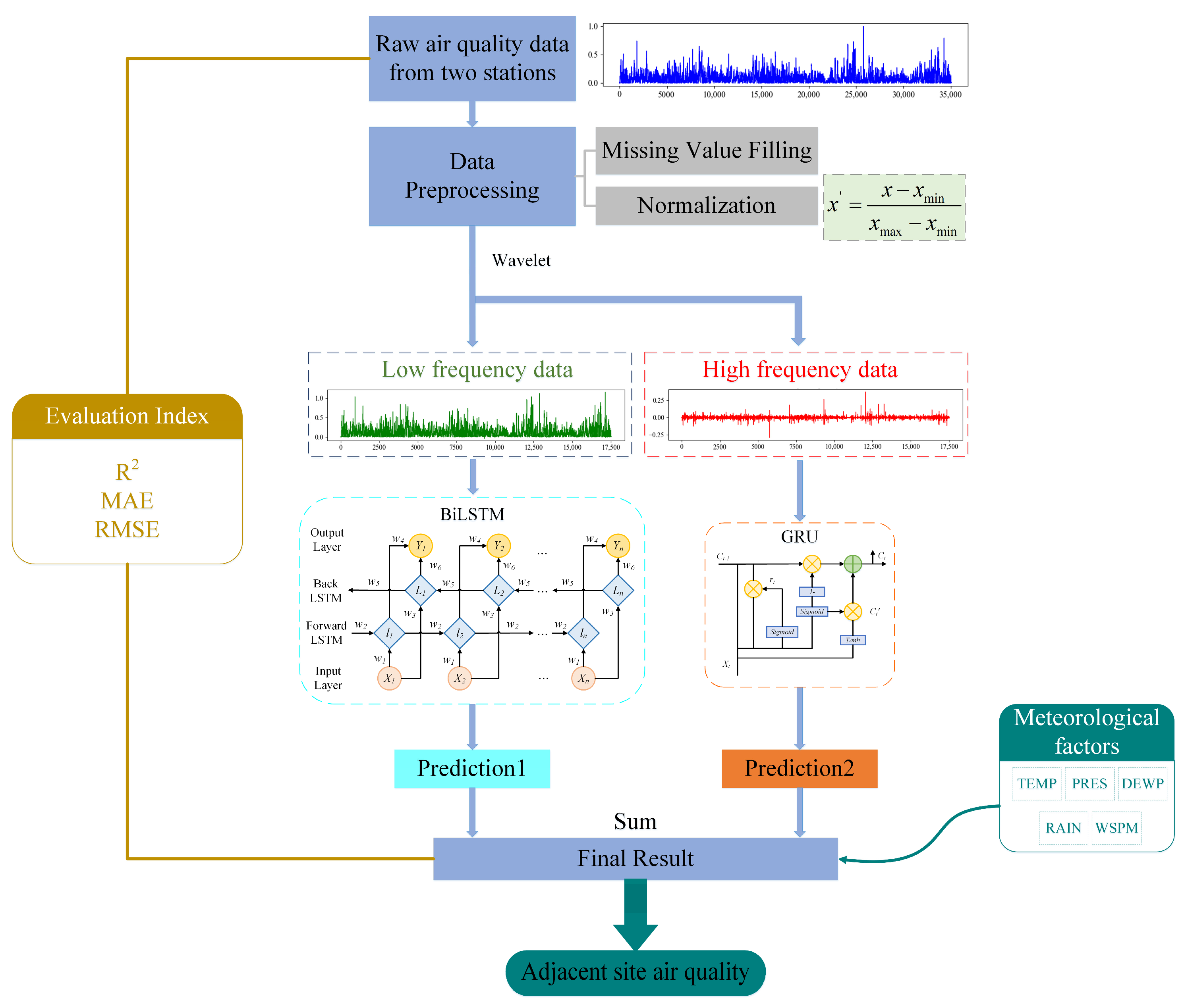
A Prediction Hybrid Framework for Air Quality Integrated with W-BiLSTM(PSO)-GRU and XGBoost Methods

Abstract

Air quality issues are critical to daily life and public health. However, air quality data are characterized by complexity and nonlinearity due to multiple factors. Coupled with the exponentially growing data volume, this provides both opportunities and challenges for utilizing deep learning techniques to reveal complex relationships in massive knowledge from multiple sources for correct air quality prediction. This paper proposes a prediction hybrid framework for air quality integrated with W-BiLSTM(PSO)-GRU and XGBoost methods. Exploiting the potential of wavelet decomposition and PSO parameter optimization, the prediction accuracy, stability and robustness was improved. The results indicate that the R² values of PM2.5, PM10, SO₂, CO, NO₂, and O₃ predictions exceeded 0.94, and the MAE and RMSE values were lower than 0.02 and 0.03, respectively. By integrating the state-of-the-art XGBoost algorithm, meteorological data from neighboring monitoring stations were taken into account to predict air quality trends, resulting in a wider range of forecasts. This strategic merger not only enhanced the prediction accuracy, but also effectively solved the problem of sudden interruption of monitoring. Rigorous analysis and careful experiments showed that the proposed method is effective and has high application value in air quality prediction, building a solid framework for informed decision-making and sustainable development policy formulation.

1. Introduction

In recent years, the global air pollution problem has become increasingly serious and has had a great impact on human health and ecological environment. Especially in China, as one of the most populous countries in the world, the air pollution problem has become more acute as a result of rapid economic development and industrialization [1]. Not coincidentally, the haze problem is also extremely serious in developed European countries such as Poland [2] and Krakow [3], due to an energy mix based on burning coal and lignite, as well as meteorological factors and topography [4]. In addition, the series of closure measures taken as a result of the novel coronavirus (COVID-19) has contributed to the significant fluctuations in air quality indicators in countries such as Brazil. Although the government has made special efforts to reduce air pollution, air pollution control is a long-term process. The World Health Organization (WHO) states that air pollution, represented by particulate matter (PM), is the main cause of premature deaths worldwide [5]. Accurately predicting air quality has evolved into a crucial imperative for proficiently managing and addressing air pollution concerns. For the public, air quality prediction can provide accurate environmental information, enabling people to take appropriate protective measures to avoid the health risks associated with long-term exposure to high pollutant concentrations. In addition, air quality forecasts not only provide real-time environmental information, but also provide strong support to governments in formulating environmental protection policies, providing public health guidance, and improving urban planning and traffic management. Nevertheless, given the intricate nature of air quality data as nonlinear time series, conventional prediction models often struggle to unravel the underlying intricate relationships concealed within the vast data, yielding suboptimal prediction outcomes. Furthermore, the issue of abrupt monitoring disruptions poses a significant hurdle in harnessing existing data comprehensively to foresee forthcoming air quality trends.

Current research in the field of air quality prediction involves both traditional methods and advanced data mining and machine learning techniques.

Huang and Cheng [6] introduced meteorological data into the AOT-PM2.5 relationship and developed multiple linear and nonlinear regression models to estimate the PM2.5 concentration in Wuhan. The results show that meteorological factors have an important influence on the AOT-PM2.5 relationship, and the multiple nonlinear regression models are better than the multiple linear models. In the study by Cobourn [7], the utilization of Nonlinear Regression (NLR) and backtracking trace concentration techniques for PM2.5 prediction revealed a significant reduction in Mean Absolute Error and a notable enhancement in prediction accuracy. Carbajal Hernandez and Sanchez-Fernandez et al. [8], and their collaborators introduced an innovative air quality assessment model incorporating the Sigma operator. This model was further enriched through the integration of a fuzzy reasoning system, leading to parameter classification and its seamless integration into the Air Quality Index, ultimately contributing to a nuanced evaluation of air pollution levels. Masseran and Safari et al. [9] employed the generalized extreme value model to dissect extreme air pollution events. Their findings illuminate a distinctive trend: an escalation in pollution severity aligned with the elongation of the return period, a phenomenon notably amplified during seasonal monsoon cycles. Moreover, classical statistical models including autoregressive (AR), moving average (MA), and autoregressive integrated moving average (ARIMA) models continue to play a pivotal role in the air quality domain for capturing and comprehending complex temporal patterns [10,11,12,13]. Numerous researchers have enhanced classical models to yield improved prediction outcomes. For instance, the seasonal autoregressive integrated moving average (SARIMA) model [14,15] was adeptly employed to establish a prediction framework for the air quality index by fully considering time factors. In pursuit of long memory air quality data monitoring, Pan and Chen [16] proposed an autocorrelation data control chart based on the autoregressive fractional integral moving average (ARFIMA) model, which efficiently maintains the data quality by taking into account the complex time dependence. Hajmohammadi and Heydecker [17] recognized the Chain Equation (MICE) method as a potent tool for achieving comprehensive data sequence completion. Building upon this foundation, a vector autoregressive moving average (VARMA) spatiotemporal model emerged, adeptly portraying the progression of air pollution. Cross-validation analysis has compellingly demonstrated that the VARMA model surpasses the spatial interpolation Kriging method and the seasonal ARMA model in efficacy, particularly for individual sites exhibiting daily or weekly trends.

While traditional air quality prediction methods have yielded some successes in certain instances, their application to predict air quality indicators using conventional statistical approaches has often fallen short. This is largely due to the intricate nature of time-series data, like PM2.5 and PM10, which exhibit high nonlinearity and instability attributed to a multitude of factors [18]. The accelerated advancement of data mining and machine learning techniques has sparked a surge of interest in leveraging these tools to enhance the precision and dependability of air quality prediction. These innovative methodologies have demonstrated remarkable efficacy in unraveling the intricate relationships and concealed patterns ingrained within PM2.5 data. Machine learning algorithms, including K-means [2], random forests [19], support vector machines [20], and neural networks [21], have gained widespread adoption for predicting PM2.5 concentrations. Their ability to adapt to non-linear data and big data greatly improves the accuracy and reliability of predictions.

Data preprocessing is an extremely important step in the data mining process. For the air quality prediction problem, more and more researchers use empirical mode decomposition (EMD), wavelet decomposition, and other techniques to preprocess the data. Huang and Yu et al. [22] introduced an air quality prediction model utilizing empirical mode decomposition (EMD) and an improved Particle Swarm Optimization (IPSO) method. Experimental outcomes highlighted substantial enhancements in predicting the Air Quality Index (AQI). Wavelet decomposition has gained traction for data augmentation in deep learning. Hu and Liu et al. [23] innovatively integrated the wavelet transform into a neural network to develop a hybrid machine learning model (WD-SA-LSTM-BP model) based on simulated annealing (SA) optimization and wavelet decomposition for PM2.5 concentration prediction. In a distinct approach, Mo and Zhang et al. [24] combined Improved Complete Ensemble Empirical Mode Decomposition with Adaptive Noise (ICEEMDAN), the Swarm Intelligence-based Whale Optimization Algorithm (WOA), and the efficient Extreme Learning Machine (ELM) to develop a comprehensive air quality early warning system. This holistic framework substantially enhances air quality prediction capabilities.

In recent years, deep learning techniques like convolutional neural networks (CNNs) and long short-term memory networks (LSTMs) have demonstrated significant potential for PM2.5 prediction [25,26]. CNNs excel at extracting spatial features, while LSTMs capture temporal patterns in PM2.5 time series, resulting in improved prediction accuracy. Composite air quality prediction frameworks, integrating various machine learning and deep learning models, have shown even more promising outcomes. For example, combining long short-term memory networks with Gated Recurrent Unit model [27], random subspace [28], attention mechanism [29], XGBoosting tree [30], random forest regression based on linear regression [31], and an adaptive fuzzy inference system with the Extreme Learning Machine [32] has yielded substantial advancements. Phruksahiran, N [33] introduced the Geographically Weighted Prediction Method (GWP), leveraging optimal machine learning algorithms and additional prediction variables. Verification using the Bangkok air quality dataset consistently outperformed conventional models across all prediction time domains. Similarly, Zhang and Wu et al. [34] integrated deep learning and multi-task learning using data from intensive air quality monitoring stations. This comprehensive model, featuring sharing and task-specific layers alongside a multi-loss joint optimization module, exhibited varied prediction performance across sites, excelling particularly when the data exhibited fluctuations and abrupt changes.

Building upon this foundation, the integration of meteorological data, satellite imagery, and other environmental factors further enhances the predictive capacity of these models. Cai and Dai et al. [35] meticulously considered the temporal dynamics of spatial pollutant concentration prediction, leveraging data from air quality and meteorological monitoring. Their work led to the creation of an automatic encoder deep network (DAEDN) denoizing model, employing a BiLSTM network that successfully extracted air quality features and performed data denoizing. Li and Peng et al. [36] adopted spatiotemporal deep learning (STDL) techniques for air quality prediction. This method concurrently forecasts air quality at all monitoring stations, capturing the temporal stability specific to each season. In comparison with spatiotemporal artificial neural networks (STANN), autoregressive moving average (ARMA), and support vector regression (SVR) models, this approach has consistently demonstrated robust predictive performance. Liu and Yan et al. [37] and team harnessed the spatiotemporal extremum learning machine (STELM) to predict air quality, attaining an impressive accuracy exceeding 80%. Sui and Han [38] devised a comprehensive multi-view, multi-task spatiotemporal map convolution network model for air quality prediction, integrating spatial, logical, and temporal viewpoints. Rigorous experimentation on real-world air quality datasets verified its superiority over existing methodologies. Liu and Lin et al. [39] and collaborators enriched the Air Quality Index time series with geographical attributes, employing a support vector machine (SVM) for predictions across uncharted spatial-temporal contexts. Their investigation underscored the significant influence of agricultural, forest usage, traffic, residential patterns, and economic factors on the Air Quality Index, while population and labor exhibited lesser correlations. Freeman and Taylor et al. [40] leveraged the recursive neural network (RNN) with LSTM architecture to predict 8 h average surface ozone (O₃) concentrations. This innovative model empowers air management professionals with real-time, continuous remote air pollution forecasts.

To mitigate local optimal traps and overfitting challenges, researchers have harnessed methodologies such as Balanced Spider Monkey Optimization (BSMO) [41], the Improved SAPSO Algorithm [42], the Tuna Swarm Optimization Model [43], and Red Deer Optimization (RDO) [44]. These techniques have been strategically applied to enhance the original model, amplifying its proficiency in air quality prediction and evaluation. Furthermore, to attain more refined predictive outcomes, numerous scholars have harmoniously amalgamated conventional techniques with neural networks for air quality prognosis.

Liu and You [45] employed both the ARIMA model and a neural network to analyze Beijing’s air pollution status and its influencing factors on the Air Quality Index (AQI). Their findings revealed that PM2.5, PM10, and O₃, the main pollutants, had the most significant impact on AQI. Moreover, the neural network model demonstrated superior prediction performance compared to the ARIMA model. When utilizing an additive seasonal model for long-term monthly data forecasting, it was observed that Beijing’s AQI still exhibits seasonal periodicity. Abu Bakar and Ariff et al. [46] devised an air quality model based on the LSTM and Autoregressive Integral Moving Average (ARIMA). Results indicated that the PM2.5 forecast using the multivariate LSTM model surpassed the performance of the single-variable LSTM model and the single-variable ARIMA model, achieving the lowest Root-Mean-Square Deviation (RMSE). Hamza and Shaiba et al. [47] and their colleagues employed the Hadoop MapReduce tool to construct a hybrid prediction model for air pollution levels, integrating ARIMA and neural networks. They optimized the performance of the mixture model using the Opposite Swallow Swarm Optimization (OSSO) algorithm and employed the Adaptive Neuro Fuzzy Inference System (ANFIS) classifier to categorize air quality into pollutant and non-pollutant states. Experimental results highlighted the enhanced predictive capabilities of the proposed ARIMA-NN method.

In summary, the limitations of traditional statistical methods in predicting PM2.5 have driven researchers to explore alternative approaches. Machine learning and deep learning algorithms have emerged as effective tools for capturing the complex dynamics of PM2.5 concentrations. By harnessing the capabilities of these methods and incorporating additional data sources, researchers are striving to develop more accurate and reliable models for PM2.5 prediction, thereby enhancing air quality management and public health interventions.

This paper aims to achieve three main objectives. Firstly, we conduct an in-depth analysis of air quality data, including correlation analysis and characterization of time-varying patterns, as a foundation for subsequent model development. Second, we propose a prediction model for air quality indicators based on the time-series fusion method of W-BiLSTM(PSO)-GRU and XGBoost. This model not only predicts air quality for known stations but also extends its predictions to unknown stations. Thirdly, we comprehensively assess the performance of the proposed model and highlight its advantages through comparative experiments with other models.

This study is organized into distinct sections. The initial section provides an overview of the research background and outlines the current landscape of air quality research. It examines the progress of related research efforts in response to the limitations of prior work. Subsequently, the second section encompasses data description, preprocessing, correlation analysis, and exploration of time-varying features within the data. We introduce various models including the discrete wavelet transform model, BiLSTM model, GRU model, PSO algorithm, XGBoost model, and the evaluation criteria. Section 3 outlines the experimental setup, research methodology, and the resulting outcomes. It presents experimental validation of the proposed model using real-world air quality data. Section 4 provides a summary of the paper, discusses the obtained results, acknowledges the limitations of the study, and suggests future research directions. Lastly, Section 5 concludes the paper by summarizing the key findings, underscoring the significance of the contributions made toward air quality research.

2. Materials and Methods

2.1. Data Description and Preprocessing

We obtained air pollution data for Beijing from the Beijing Ecological Environment Testing Center (http://www.bjmemc.com.cn/, accessed on 1 May 2023). The meteorological data are from the China Surface Meteorological Dataset of the National Meteorological Information Center (http://data.cma.cn/, accessed on 1 May 2023). For the numerous monitoring stations in Beijing, this paper selects the aotizhongxin and xichengguanyuan stations for subsequent experiments in order to facilitate model validation, and the geographic location map is shown in Figure 1. We selected the air pollution dataset consisting of PM2.5, PM10, SO₂, CO, NO₂, and O₃ and the meteorological dataset consisting of ambient temperature, air pressure, dew point temperature, precipitation, and wind speed in Beijing from 2013–2017. Both air quality data and meteorological data are recorded hour by hour, with a time interval of 1 h, totaling 35,064 data.

Table 1. Air Quality and Meteorological Dataset for the Aotizhongxin site.

Day	Month	Year	Hour (h)	PM2.5 (μg·m−3)	PM10 (μg·m−3)	SO2 (μg·m−3)	NO2 (μg·m−3)	CO (μg·m−3)	O3 (μg·m−3)	TEMP (°C)	PRES (hpa)	DEWP (°C)	RAIN (mm)	WSPM (m/s)
01	03	2013	0	4	4	4	7	0.3	77	−0.7	1023	−18.8	0	4.4
01	03	2013	1	8	8	4	7	0.3	77	−1.1	1023.2	−18.2	0	4.7
…			…	…	…	…	…	…	…	…	…	…	…	…
…			…	…	…	…	…	…	…	…	…	…	…	…
26	06	2015	2	108	108	2	12	0.5	152	21.1	995.6	19.4	5.3	0.7
26	06	2015	3	104	104	2	16	0.6	130	20.8	995.7	19.6	9.6	0.3
…			…	…	…	…	…	…	…	…	…	…	…	…
28	02	2017	22	21	44	12	87	0.7	35	10.5	1014.4	−12.9	0	1.2
28	02	2017	23	19	31	10	79	0.6	42	8.6	1014.1	−15.9	0	1.3

TEMP refers to ambient temperature, PRES to air pressure, DEWP to dew point temperature, RAIN to precipitation, and WSPM to wind speed.

shows some of the datasets.

The presence of missing values and inhomogeneous dimensions in various AQI data affects the accuracy of model predictions. Considering the dispersed nature of air pollutants, this paper uses the average of two nearby stations at the same time to fill in the missing values. On this basis, for the missing data of the three stations, cubic spline interpolation is used to fill them.

Cubic spline interpolation uses multiple low-order polynomials across all data points and refines the cubic spline curve using a third-order polynomial between two data points rather than a linear function of the linear spline curve between the two points. Also, the smoothness of the junction points is ensured by connecting them with second-order continuous derivatives. As a result, cubic spline curve interpolation can maximally simulate the evolution process of gradual change of physical phenomena, leading to the ideal interpolation effect [48].

This paper normalized all data by min-max and the conversion function is shown in Equation (1), where $x_{\max }$ is the maximum value of the data, and $x_{\min }$ is the minimum value of the data. This was by far the most common method of data standardization.

$$x^{\prime }=\frac{x-x_{\min }}{x_{\max }-x_{\min }}$$

(1)

2.2. Correlation Analysis

Correlations between different features in the dataset can lead to feature redundancy. Additionally, not all influencing factors are directly related to air quality. The purpose of correlation analysis is to investigate the relationships between air quality indicators and meteorological factors, essentially conducting a preliminary examination of other variables associated with air quality.

This study used Pearson correlation analysis to determine the relationship between air quality indicators and weather factors. In the absence of significant correlation, the meteorological factors should not be chosen as independent variables for predicting air quality. The heat plots of correlation coefficients between AQIs and meteorological factors for the aotizhongxin and xichengguanyuan sites from 2013 to 2017 are shown in Figure 2 and Figure 3.

The correlation heatmap revealed several significant patterns and correlations between AQIs and meteorological factors. Firstly, we observe a high positive correlation between PM2.5 and PM10, suggesting a common source of particulate matter pollution. Second, sulphur dioxide was moderately positively correlated with PM2.5, PM10, and nitrogen dioxide, suggesting the potential role of sulphur dioxide in secondary aerosol formation. Thirdly, carbon monoxide showed strong positive correlation with PM2.5, PM10, and nitrogen dioxide, suggesting that vehicular emissions are a common source. Fourthly, ozone was negatively correlated with PM2.5, PM10, SO₂, NO₂, CO, indicating complex interactions between ozone and other pollutants. Finally, meteorological factors such as temperature and wind speed showed varying degrees of correlation with different AQIs, suggesting that they influence the dispersion and chemical reactions of pollutants. For example, as can be seen in Figure 2 and Figure 3, PM2.5 shows a weak negative correlation with air temperature, a very weak correlation with pressure, a weak positive correlation with dew point temperature, a weak negative correlation with precipitation, and a weak negative correlation with wind speed.

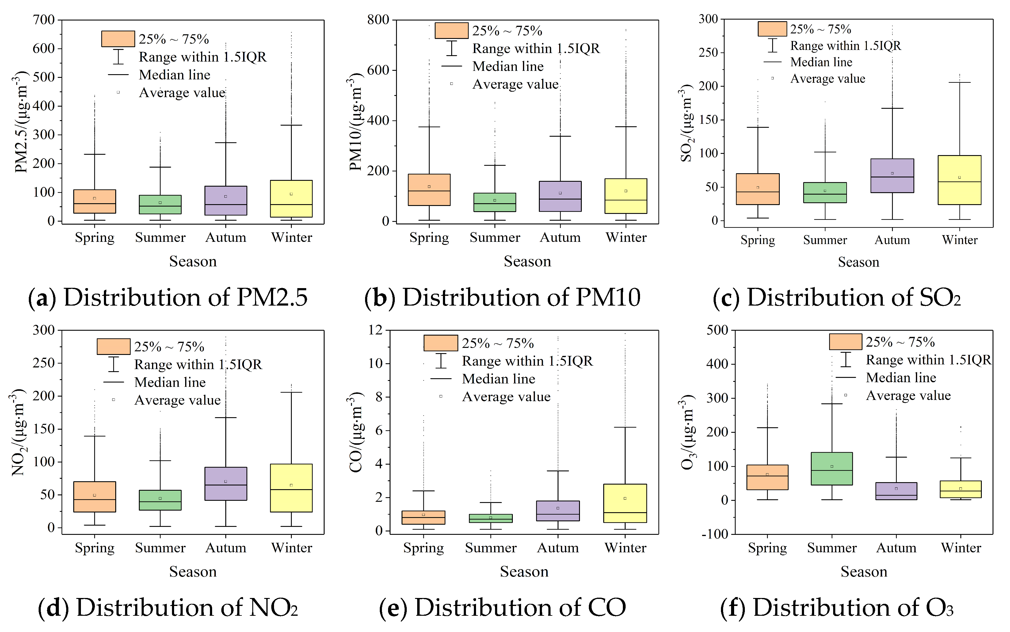
2.3. Characterization of Temporal Changes in Contamination

The concentration of PM2.5 exhibits distinct seasonal variations attributed to emissions from pollution sources and meteorological conditions. Figure 4 illustrates the seasonal distribution of PM2.5, PM10, SO₂, NO₂, CO, and O₃ concentrations at the aotizhongxin and xichengguanyuan sites in Beijing from 2013 to 2017. In accordance with Beijing City’s actual context, the analysis designates March to May as spring, June to August as summer, September to November as fall, and December, January, and February as winter. Figure 5 showcases the seasonal distribution of the six AQIs, encompassing mean, median, maximum, and anomalies, with the aotizhongxin site as the reference. Figure 4 reveals that PM2.5 and PM10 concentrations in Beijing primarily exhibit a higher distribution during winter, followed by spring and autumn, and a lower concentration in summer. This pattern emerges due to the winter’s lower temperatures, less favorable meteorological diffusion conditions, and the long-range transmission of atmospheric pollutants emitted during the heating season, leading to the accumulation of PM2.5 in the near-surface atmosphere. Spring and fall experience improved atmospheric diffusion conditions compared to winter, but their dry weather conditions hinder the secondary generation of PM2.5. In contrast, summer, characterized by frequent rainfall and better meteorological diffusion, facilitates PM2.5 dispersion and removal.

SO₂ content demonstrates significant variability, forming a “V” shape, with elevated concentrations during winter. This phenomenon can be attributed to increased industrial emissions and fuel consumption, particularly coal, in the colder months. Additionally, unfavorable meteorological conditions during winter impede the chemical transformation of SO₂, prolonging its atmospheric presence. Conversely, the influence of summer’s increased rainfall leads to a reduction in SO₂ content, as a substantial amount is washed out through precipitation. The aotizhongxin and xichengguanyuan sites exhibit multi-year average peaks of approximately 24.4 mg/m³ and 25.6 mg/m³, respectively, and minimum values around 5.0 mg/m³. NO₂ displays pronounced seasonal fluctuations, registering lower concentrations in summer and higher levels in winter. This trend indicates significant anthropogenic emissions of NO₂ in the aotizhongxin and xichengguanyuan areas. In regions dominated by natural sources, NO₂ concentration peaks during summer, attributed to lightning processes and soil emissions. Conversely, in areas influenced by anthropogenic sources, the highest NO₂ levels occur in winter [49], where emission increases and poor diffusion conditions contribute to elevated winter NO₂ concentrations in Beijing.

Ozone pollution remains relatively mild during winter due to consistently high temperatures and abundant sunshine. Favorable conditions for the photochemical reaction of atmospheric nitrogen oxides (NO_x) and volatile organic compounds (VOCs) to produce surface ozone contribute to this pattern [50]. Lower temperatures, reduced hours of sunshine, increased solar radiation intensity, and wind speeds in the winter months combined to result in an overall decrease in ozone concentrations of about 65 mg/m³ compared to the summer months. The CO concentration in Beijing demonstrates a distinct seasonal pattern. It remains low during June to August, stabilizing at 0.85 mg/m³ at both stations, before a rapid increase from September to November and reaching its yearly peak during December to February. The discernible correlation between the CO concentration fluctuations and the temperature underscores the temperature’s crucial role in shaping the seasonal variation of NO₂ column concentrations.

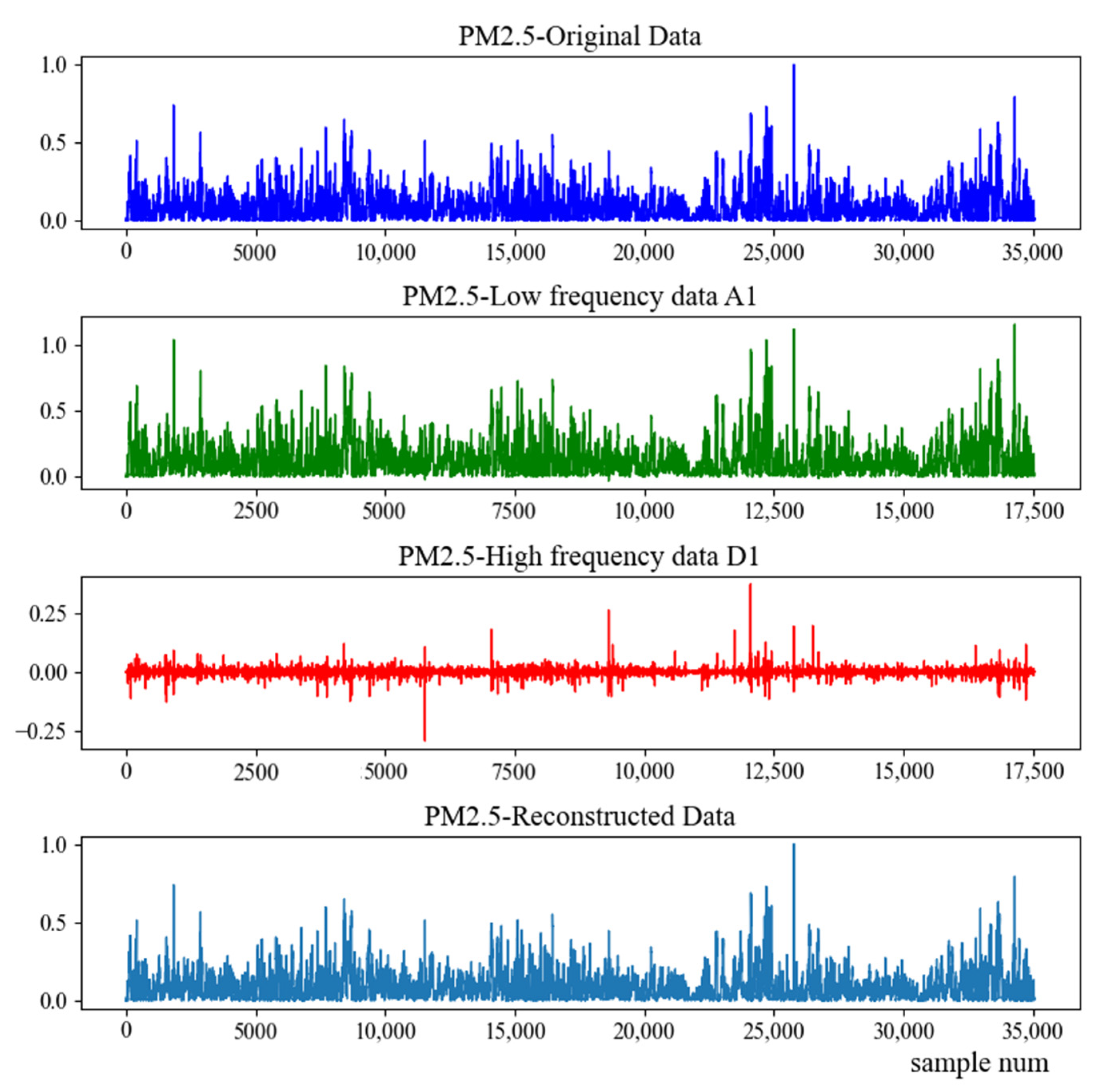
2.4. Wavelet Transform

The original AQI dataset is influenced by multiple factors and contains extremely frequent and dramatic fluctuations. Without data preprocessing, it is difficult to obtain good learning and prediction results by deep learning modeling these alone. Wavelet transform is a time-frequency analysis of signals designed to perform multiscale analysis of time-series signals in both time and frequency domains [51], and it is often widely used to deal with the problem of signal-to-noise separation of such time-series data. With good localization properties in both the time and frequency domains, it can focus on any details of an object by applying progressively finer sampling steps to the high-frequency components in either the time or frequency domain. The raw air quality data can be viewed as a nonsmooth, nonlinear time series, which can be decomposed by m-level wavelet transform decomposition [52]:

$$y(t)=A_m(t)+{\displaystyle {\sum }_{i=1}^m{D}_i(t)}$$

(2)

where $A_m$ is the low-frequency information set that represents the general trend of air quality, and $D_i$ is the high-frequency information set that represents the random perturbations in the air quality data, which is the noise portion of the raw data.

Commonly used wavelet functions are haar wavelet, db wavelet, morlet wavelet, marr wavelet, etc. In this study, “db4” wavelet is chosen to decompose the original data into two sub-sequences of low-frequency component A1 with weak volatility and high-frequency component D1 with strong volatility. Using the decomposed sequence to restore the original sequence is wavelet reconstruction. Taking the aotizhongxin site as an example, the decomposition and reconstruction results of the air quality indicator PM2.5 are shown in Figure 6.

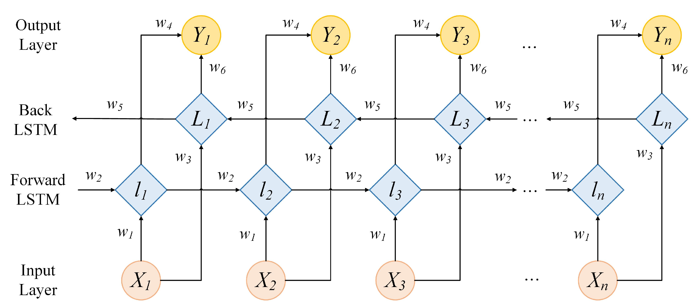
2.5. Bidirectional Long Short-Term Memory (BiLSTM)

The LSTM network, a type of recurrent neural network, comprises forward LSTM and backward LSTM components [53], effectively addressing the gradient explosion or vanishing issues present in conventional recurrent neural networks. Building upon the foundation of traditional RNN, LSTM introduces forgetting gates, input gates, and output gates, which enables the model to maintain a more consistent error during backpropagation and facilitates continuous learning across multiple time steps. This enhancement significantly improves the accuracy of time-series predictions. BiLSTM, an extension of LSTM [54], incorporates an additional inverse operation that surpasses LSTM in capturing the intricate relationships within sequence features, leading to even more precise time series predictions. The architecture of BiLSTM is illustrated in Figure 7.

Where $X_1,X_2,\dots ,X_i$ are the corresponding input data at each moment from $t_1$ to $t_i(i\in [1,t])$, respectively, and $Y_1,Y_2,\dots ,Y_i$ denote the corresponding output data. $l_1,l_2,\dots ,l_i$ represent the forward iterative LSTM hidden states at each moment, and $L_1,L_2,\dots ,L_i$ for indicate the backward iterative LSTM hidden states. $w_1,w_2,\dots ,w_i$ stand for the corresponding weights of each layer. The calculation formulas of the final output process of BiLSTM are shown in Equations (3)–(5):

$$l_i=f_1(w_1{X}_i+w_2{l}_{i-1})$$

(3)

$$L_i=f_2(w_3{X}_i+w_5{L}_{i+1})$$

(4)

$$Y_i=f_3(w_4{l}_i+w_6{L}_i)$$

(5)

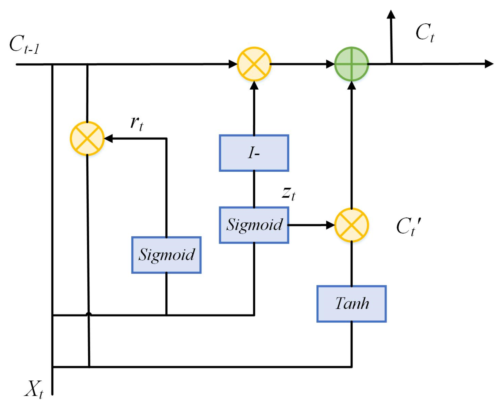
2.6. Gated Recurrent Unit (GRU)

Different from the architecture of LSTM, GRU optimizes the three gate functions by combining the forgetting gate and the input gate into a single unified update gate, which is a simplification of the LSTM network structure [55]. By doing so, it reduces the parameter count within LSTM network units, consequently shortening the model’s training duration. The update gate plays a pivotal role in determining how much past state information is retained in the current state. A higher update gate value signifies greater retention of previous state information. Meanwhile, the reset gate is responsible for deciding whether a prior computational state should be forgotten. A lower reset gate value corresponds to more information being disregarded. The architecture of the BiLSTM is depicted in Figure 8, where $X_t$, $C_t$, $r_t$, $z_t$, and $C_t\prime$ are the input vector, state memory variable, reset gate state, update gate state, and current setup candidate state, respectively, at moment t. I denotes the unit matrix. The expression is given by Equations (6)–(9):

$$z_t=\sigma (W_z\cdot [C_{t-1},X_t])$$

(6)

$$r_t=\sigma (W_r\cdot [C_{t-1},X_t])$$

(7)

$$C_t\prime =\tanh (W_c\cdot [r_t\times C_{t-1},X_t])$$

(8)

$$C_t=(1-z_t)\times C_{t-1}+z_t\times C_t\prime$$

(9)

where $W_z$, $W_r$, $W_c$, and $W_o$ are the weight parameters and $\sigma$ denotes the sigmoid activation function.

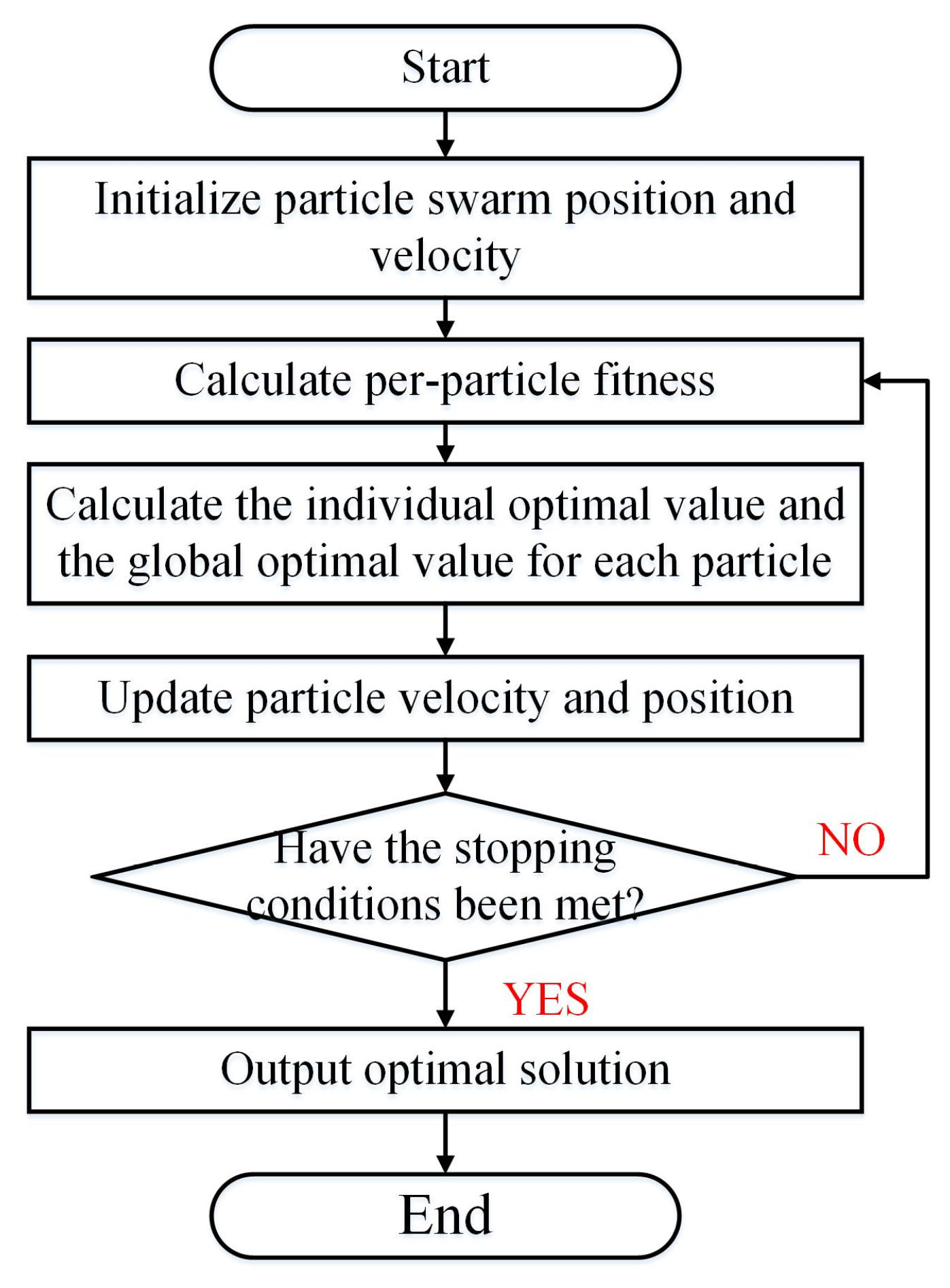
2.7. Particle Swarm Algorithm (PSO)

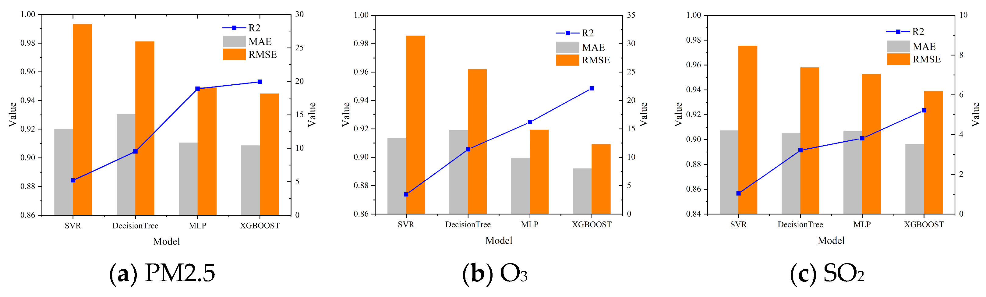
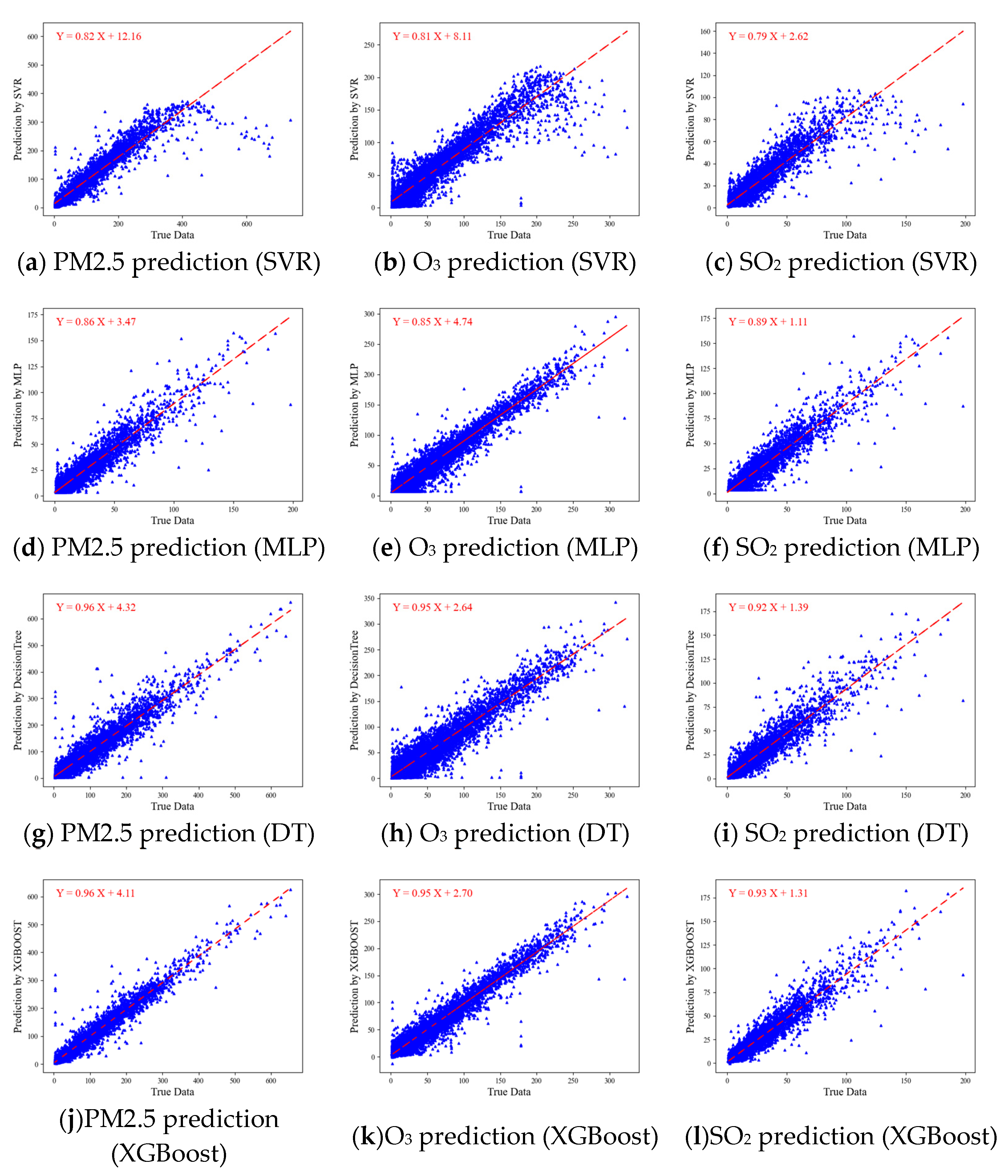
The Particle Swarm Optimization (PSO) algorithm [56], which draws inspiration from the feeding behavior of bird flocks and mimics the stochastic search and intelligent optimization of natural organisms, is a widely used method for optimizing complex numerical functions. In PSO, the search space consists of an infinite number of particles, each trying to optimize a fitness function. Each particle calculates its fitness value based on its position in the search space. Using information about its current position and past optimal positions, the direction of movement is determined. These steps are repeated until a predetermined termination criterion is met. In this study, the PSO algorithm was integrated with the BiLSTM neural network model to determine the optimal number of layers and neurons for the BiLSTM model. This integration automatically determines the optimal number of network layers and the number of neurons per layer. The flowchart of the PSO algorithm is shown in Figure 9.

2.8. XGBoost

This study utilizes the XGBoost algorithm for air quality prediction. XGBoost is a scalable tree boosting machine learning framework [57], applicable to solving various machine learning tasks including classification and regression. The algorithm employs multiple trees to collectively learn and predict outcomes, operating within the gradient boosting framework. The core concept involves iteratively adding new regression trees while adjusting for the residuals of the preceding model through newly generated CART trees. The sum of the results from each tree contributes to the final prediction [58]. XGBoost leverages first-order and second-order derivatives to enhance prediction accuracy and incorporates regularization to prevent overfitting [59]. Moreover, XGBoost supports parallel tree operations, approximate tree construction, processing of sparse data, and optimized memory usage. This results not only in high prediction accuracy but also in significant computational efficiency. As a result, XGBoost has gained widespread use in diverse data analysis and mining competitions.

The objective function of XGBoost is defined as:

$$Obj={\displaystyle \sum _{i=1}^{N}l(y_i,y_i\prime )}+{\displaystyle \sum _{i=1}^K\mathsf{\Omega }(f_k)}$$

(10)

where the first term is the training loss function and the second term is a regularization term to prevent overfitting, represented by Equation (11):

$$\mathsf{\Omega }(f_k)=\gamma T+\frac{1}{2}\lambda {‖w‖}^2$$

(11)

$l$ is the loss function, $T$ denotes the number of leaf nodes, $\gamma$ and $\lambda$ are the complexity parameter and penalty factor, respectively. $w$ denotes the weight of the leaf node, $y_i$ is the true value of the sample, $y_i\prime$ is the final predicted value of the model, defined as:

$$y_i\prime ={\displaystyle \sum _{k=1}^K{f}_k(x_i)}$$

(12)

where $x_i$ is the input variable, $K$ is the number of regression trees, and $f_k$ is the kth tree model.

2.9. Model Evaluation Metrics

To comprehensively assess the classification performance of various models across different levels, this study evaluates the predictive outcomes using metrics such as Root-Mean-Square Error (RMSE), Mean Absolute Error (MAE), and R-squared (R²) values.

MAE quantifies the disparity between predicted and actual values, with smaller values indicating superior performance. The formula for calculating MAE is presented as follows in Equation (13):

$$MAE=\frac{1}{n}{\displaystyle \sum _{i=1}^n|{\widehat{y}}_i-y_i|}$$

(13)

The RMSE is highly sensitive to errors in the magnitude of prediction results within the training set, making it a valuable indicator of prediction accuracy. A smaller RMSE value signifies better performance. The formula for calculating RMSE is presented in Equation (14).

$$RMSE=\sqrt{\frac{1}{n}{\displaystyle \sum _{i=1}^n{\left({\widehat{y}}_i-y_i\right)}^2}}$$

(14)

The R² score, also referred to as the coefficient of determination, assesses the goodness-of-fit between the predicted values and the actual observed values. Its optimal value, with an upper limit of 1, can also assume negative values. A score closer to 1 signifies a stronger alignment between predictions and observations, indicating superior predictive performance. The calculation formula for R² is depicted in Equation (15):

$$R^2=1-\frac{{\displaystyle \sum _{i=1}^n{\left({\widehat{y}}_i-y_i\right)}^2}}{{\displaystyle \sum _{i=1}^n{\left({\overline{y}}_i-y_i\right)}^2}}$$

(15)

In this context, $y_i$ represents the actual value of the ith data point; ${\widehat{y}}_i$ represents the corresponding predicted value; and ${\overline{y}}_i$ signifies the mean value of the time series. Typically, the coefficient of determination, R², varies between 0 and 1. An R² value of 0 indicates that the model is unable to predict the target variable, while an R² value of 1 suggests a flawless prediction. Negative R² values can also occur, indicating that the model’s predictive capability is weaker than directly calculating the mean of the target variable.

3. Results

3.1. Experiments Settings

In this paper, we employed a chronological division of the dataset into a training set and a test set, maintaining a ratio of 7:3. Considering both computational efficiency and prediction accuracy, data from 36 time points are selected as inputs for modeling, allowing for the prediction of pollutant concentrations at subsequent moments. The BiLSTM and GRU parameter settings are shown in

Table 2. Parameter description of BiLSTM.

Parameter	Value
Number of layers	3
Number of neurons per layer	135
Optimizer	Adam
Learning rate	0.01
Activation function	Relu
Loss function	Mean_absolute_error
Batch_size	94
Epochs	50
Dropout	0.16

and

Table 3. Parameter description of GRU.

Parameter	Value
Number of layers	2
Number of neurons per layer	150
Optimizer	Adam
Learning rate	0.01
Activation function	Relu
Loss function	Mean_absolute_error
Batch_size	32
Epochs	50
Dropout	0.2

.

Throughout the training process, the BiLSTM model utilizes the “Adam” optimization algorithm and the “Mean Squared Error” loss function. Although the model’s predictive performance hinges on factors like neural network depth and neuron counts per layer, parameter tuning traditionally relies on human intervention, posing challenges in achieving optimal configurations. To tackle this, we implemented the neural network framework using Python alongside its deep learning libraries, Tensorflow and Keras. Leveraging the Particle warm Optimization (PSO) algorithm, we pursued parameter optimization to attain the optimal prediction efficacy of the BiLSTM neural network. In tandem, we designed controlled experiments encompassing various parameter setups, fostering a comprehensive understanding of the proposed model’s prediction capabilities across diverse zones within Beijing. All experiments were implemented using Python software (3.10) on a computer with an Inter Core(TM) i7-8809G CPU, 16 GB of memory, and a Windows 11 64-bit system.

3.2. Air Quality Prediction Model

Taking the PM2.5 indicator as an example, firstly, wavelet decomposition of the PM2.5 sequence is performed to separate the PM2.5 data into low-frequency components and high-frequency components, which are then utilized as the input variables of the BiLSTM network and the GRU network, respectively. Typically, noise is predominantly concentrated in the high-frequency components, while the low-frequency components are less susceptible to noise interference. However, complete noise removal can substantially diminish prediction accuracy. Consequently, all original sequence components were preserved following wavelet decomposition. Subsequently, the BiLSTM-GRU prediction model was employed to generate forecasted values for each component. Ultimately, the predictions from each component were amalgamated to yield the ultimate prediction outcomes.

The accuracy of fitting complex data is hindered by too few neural network layers, whereas an excess of layers increases model intricacy. Additionally, the uncertainty associated with manually set parameters necessitates an alternate approach. Hence, we employed the PSO algorithm to determine the optimal number of layers and neurons for the BiLSTM model. The optimized model yielded enhanced R-squared values and diminished MAE and RMSE values, underscoring that the utilization of the PSO algorithm for optimizing the BiLSTM neural network led to heightened prediction accuracy. Figure 10 shows the architecture of the model.

3.3. Prediction Model Validation and Sustainability Analysis

To assess the model’s effectiveness, the air quality dataset provided by the Beijing Ecological Environment Monitoring Center for the years 2013 to 2017 was utilized to validate the Air Quality Index (AQI) prediction model. Six key air quality indicators, namely PM2.5, PM10, SO₂, NO₂, CO, and O₃, were employed as time-series data for validation purposes. To ascertain the model’s efficacy, ablation experiments were conducted to compare its performance.

For enhanced clarity in evaluating the model’s performance, this study employed two specific monitoring sites, namely aotizhongxin and xichengguanyuan, as case examples. A comprehensive comparison of the models’ performance is presented in

Table 4. Prediction results of each model at the aotizhongxin site.

Site	Experimental Indicators	Model	R2	MAE	RMSE
aotizhongxin	PM2.5	SVR	0.8754	0.0008	0.0289
		Random Forest	0.9354	0.0110	0.0232
		LSTM	0.9409	0.0137	0.0253
		BiLSTM	0.9429	0.0129	0.0249
		W-BiLSTM	0.9450	0.0147	0.0244
		W-BiLSTM-GRU	0.9537	0.0113	0.0224
		W-BiLSTM(PSO)-GRU	0.9747	0.0076	0.0158
	PM10	SVR	0.8920	0.0004	0.0196
		Random Forest	0.8625	0.0195	0.0389
		LSTM	0.9029	0.0113	0.0189
		BiLSTM	0.9078	0.0097	0.0184
		W-BiLSTM	0.9237	0.0085	0.0137
		W-BiLSTM-GRU	0.9318	0.0076	0.0129
		W-BiLSTM(PSO)-GRU	0.9572	0.0058	0.0100
	SO2	SVR	0.8127	0.0006	0.0246
		Random Forest	0.8986	0.0111	0.0215
		LSTM	0.8918	0.0082	0.0156
		BiLSTM	0.9050	0.0077	0.0146
		W-BiLSTM	0.9242	0.0070	0.0131
		W-BiLSTM-GRU	0.9291	0.0065	0.0126
		W-BiLSTM(PSO)-GRU	0.9421	0.0045	0.0116
	NO2	SVR	0.7545	0.0031	0.055
		Random Forest	0.8440	0.0357	0.0506
		LSTM	0.8996	0.0268	0.0427
		BiLSTM	0.9040	0.0256	0.0417
		W-BiLSTM	0.9263	0.0256	0.0366
		W-BiLSTM-GRU	0.9355	0.0223	0.0342
		W-BiLSTM(PSO)-GRU	0.9770	0.0143	0.0198
	CO	SVR	0.7969	0.0023	0.0478
		Random Forest	0.8881	0.0223	0.0424
		LSTM	0.9118	0.0226	0.0477
		BiLSTM	0.9167	0.0255	0.0464
		W-BiLSTM	0.9458	0.0201	0.0374
		W-BiLSTM-GRU	0.9461	0.0215	0.0373
		W-BiLSTM(PSO)-GRU	0.9771	0.0119	0.0226
	O3	SVR	0.7443	0.0028	0.0533
		Random Forest	0.8367	0.0349	0.0539
		LSTM	0.9195	0.0243	0.0361
		BiLSTM	0.9225	0.0225	0.0355
		W-BiLSTM	0.9310	0.0227	0.0335
		W-BiLSTM-GRU	0.9383	0.0202	0.0317
		W-BiLSTM(PSO)-GRU	0.9852	0.0107	0.0159

and

Table 5. Prediction results of each model at the xichengguanyuan site.

Site	Experimental Indicators	Model	R2	MAE	RMSE
xichengguanyuan	PM2.5	SVR	0.8779	0.0014	0.0370
		Random Forest	0.9261	0.0191	0.0321
		LSTM	0.9468	0.0166	0.03165
		BiLSTM	0.9502	0.0161	0.0306
		W-BiLSTM	0.9612	0.0146	0.0270
		W-BiLSTM-GRU	0.9697	0.0158	0.0238
		W-BiLSTM(PSO)-GRU	0.9707	0.0125	0.0226
	PM10	SVR	0.7498	0.0015	0.0389
		Random Forest	0.8951	0.0154	0.0289
		LSTM	0.9073	0.0177	0.0313
		BiLSTM	0.9135	0.0166	0.0302
		W-BiLSTM	0.9330	0.0161	0.0266
		W-BiLSTM-GRU	0.9337	0.0151	0.0264
		W-BiLSTM(PSO)-GRU	0.9658	0.0108	0.0186
	SO2	SVR	0.7944	0.0009	0.0305
		Random Forest	0.8177	0.0172	0.0358
		LSTM	0.8254	0.0092	0.0236
		BiLSTM	0.8324	0.0088	0.0231
		W-BiLSTM	0.8523	0.0081	0.0217
		W-BiLSTM-GRU	0.9185	0.0084	0.0162
		W-BiLSTM(PSO)-GRU	0.9450	0.0055	0.0133
	NO2	SVR	0.7524	0.0032	0.0562
		Random Forest	0.8533	0.0353	0.0506
		LSTM	0.9111	0.0263	0.0403
		BiLSTM	0.9117	0.0255	0.0402
		W-BiLSTM	0.9162	0.0290	0.0391
		W-BiLSTM-GRU	0.9343	0.0231	0.0347
		W-BiLSTM(PSO)-GRU	0.9792	0.0131	0.0194
	CO	SVR	0.8298	0.0013	0.0367
		Random Forest	0.8768	0.0186	0.0351
		LSTM	0.9135	0.0172	0.0347
		BiLSTM	0.9200	0.0173	0.0334
		W-BiLSTM	0.9290	0.0217	0.0314
		W-BiLSTM-GRU	0.9467	0.0152	0.0272
		W-BiLSTM(PSO)-GRU	0.9759	0.0097	0.0174
	O3	SVR	0.7642	0.0025	0.0497
		Random Forest	0.8394	0.0333	0.0560
		LSTM	0.9087	0.0227	0.0359
		BiLSTM	0.9125	0.0168	0.0304
		W-BiLSTM	0.9251	0.0209	0.032
		W-BiLSTM-GRU	0.9281	0.0191	0.0318
		W-BiLSTM(PSO)-GRU	0.9726	0.0133	0.0201

, providing a more tangible understanding of the model’s predictive prowess and its superiority in predicting air quality indicators. Employing data from the aotizhongxin monitoring station, we obtained predicted values from seven distinct models: SVR, Random Forest, LSTM, BiLSTM, W-BiLSTM, W-BiLSTM-GRU, and W-BiLSTM(PSO)-GRU. Through rigorous comparison with actual values and subsequent error calculations, we derived the experimental outcomes. As illustrated in Table 4 for the aotizhongxin site, the proposed models achieved R² values of 0.9747, 0.9572, 0.9421, 0.9770, 0.9771, and 0.9852 for the six studied parameters, respectively, outperforming their counterparts. The resultant minimized MAE and RMSE values reinforce the superior predictive capacity of the W-BiLSTM(PSO)-GRU model in extracting crucial features from air quality data and forecasting air quality indicators with enhanced precision.

As evident from the comparative visualization of prediction outcomes, deep learning models exhibit superior predictive capabilities compared to traditional machine learning models like SVR and random forest. Notably, LSTM and GRU models demonstrate enhanced predicted R² values and reduced MAE and RMSE values, indicating their improved accuracy. Upon incorporating wavelet decomposition, both LSTM and BiLSTM models showcase refinement in their predictions, displaying higher R² values and diminished MAE and RMSE values. This enhancement underscores the positive impact of integrating wavelet decomposition into the analysis of non-stationary time-series data. Furthermore, by replacing the LSTM model with BiLSTM and GRU models for predicting the decomposed low-frequency and high-frequency terms, respectively, substantial improvements in R² values are observed, accompanied by significant reductions in MAE and RMSE values compared to the previous models. Remarkably, the W-BiLSTM(PSO)-GRU model excels across all six metrics, surpassing an R² value of 0.94 and maintaining MAE and RMSE values below 0.02 and 0.03, respectively. This substantiates the pronounced advantages of this model.

In the scope of this study, we have provided a comprehensive analysis of air quality dynamics through the precise forecasting of six pivotal air quality indicators: PM2.5, PM10, SO₂, NO₂, CO, and O₃, across two distinct air quality monitoring stations. Building upon this foundational insight, we have incorporated meteorological factors into our air quality prediction framework. By leveraging the forecasted values from the initial two stations, we have extended our investigation to predict air quality trends at neighboring monitoring stations. This innovative methodology effectively addresses potential disruptions in monitoring operations. Leveraging data from proximate monitoring stations, we have established a continuous and reliable forecasting framework, even in scenarios involving site-specific interruptions.

This research has employed the XGBoost model for air quality prediction, with detailed core parameters elucidated in

Table 6. Parameter description of XGBoost.

Parameter	Value
learning_rate	0.08
n_estimators	300
gamma	0.07
min_child_weight	1
subsample	1
max_depth	3
min_child_weight	1
n_jobs	1
max_delta_step	0
reg_alpha	0
reg_lambda	1
colsample_bytree	1

. Comprehensive experimental analyses encompassed the SVR, decision tree, MLP, and XGBoost models. These analyses harnessed Air Quality Index (AQI) data from neighboring sites, accompanied by the respective meteorological factors of the predicted sites, as input variables. The AQIs of the sites under consideration were employed as dependent variables. Model performance evaluation encompassed three pivotal metrics: R-squared (R²), Mean Absolute Error (MAE), and Root-Mean-Square Error (RMSE). Illustratively, for the aotizhongxin site, exemplified with the PM2.5, O₃, and SO₂ indicators, the experimental findings are visually depicted in Figure 11 and Figure 12.

In the comparison of overall algorithm performance, a distinct trend in their predictive capabilities emerges. The SVR algorithm demonstrates a moderate level of accuracy, yielding an R² value of 0.8843 for PM2.5, along with MAE and RMSE values of 12.87 and 28.53, respectively. This suggests a reasonable correlation between predicted and actual PM2.5 values. While DecisionTree exhibits improved correlation, it comes with a slightly higher prediction error. Notably, the Multilayer Perceptron (MLP) algorithm demonstrates a significant enhancement in prediction accuracy, effectively capturing potential underlying patterns. However, it is the Extreme Gradient Boosting (XGBoost) algorithm that shines, boasting the highest correlation and the lowest prediction error. For PM2.5, XGBoost achieves an impressive R² value of 0.9530, an MAE value of 10.40, and an RMSE value of 18.19. From a holistic standpoint, MLP and XGBoost outperform SVR and Decision Tree in terms of predictive capabilities. These advanced machine learning techniques, particularly XGBoost, hold promising prospects for accurate PM2.5 prediction. This comparison underscores the significance of employing modern algorithms to enhance air quality prediction, emphasizing the potential for refined environmental management and targeted public health interventions. In summary, a discernible pattern in predictive proficiency is evident among these algorithms.

Air quality prediction, as an effective way to improve air quality management, is most directly aimed at informing the public about the environmental quality and air quality and making preparations in advance to cope with the situation, so as to ensure that human beings can live sustainably while satisfying their basic needs. The above experimental results fully demonstrate that the hybrid prediction framework fusing W-BiLSTM(PSO)-GRU and XGBoost proposed in this paper basically achieves accurate prediction of air quality, which can help to protect people’s health and sustainable development of the ecological environment.

4. Discussion

In recent years, air quality issues have significantly impacted public health and daily life, making air quality prediction a critical research area. The complexity of factors influencing air quality, such as PM2.5, PM10, SO₂, NO₂, CO, O₃, and other air quality indicators, results in data that exhibits complexity and non-stationarity. However, as complexity increases, traditional time-series models demonstrate limited generalization performance for highly volatile time-series data, posing a challenge in accurately predicting pollution. To address this, we propose a comprehensive prediction model based on W-BiLSTM(PSO)-GRU, which proves highly adaptable for air quality prediction across diverse environments. Firstly, this paper adopts the wavelet analysis method to separate the low-frequency components from the high-frequency components of the time series of air quality indicators. Subsequently, we employed deep learning models to separately capture the characteristics of these components and then fused the final prediction results, enhancing our ability to analyze nonlinear and non-smooth data patterns. Traditional LSTM represents a widely employed time-series prediction technique, an evolution of RNN. Building upon this, BiLSTM introduces a bidirectional architecture that incorporates both past and future information, enhancing its capacity to handle sequential data. To further enhance prediction accuracy, we optimized the parameters of the BiLSTM network using the PSO algorithm. Additionally, the GRU model, compared to LSTM, presents a streamlined parameter configuration, facilitating seamless fusion.

It is shown that for the two sites, aotizhongxin and xichengguanyuan, the LSTM neural network model is more effective in predicting the air quality time series than the traditional machine learning models such as SVR and random forest. On this basis, the introduction of BiLSTM, GRU network, and wavelet decomposition can further improve the prediction value of R², while the MAE and RMSE values are decreased. For example, for the PM2.5 indicator at the aotizhongxin site, the W-BiLSTM-GRU model improves the R² value by 0.0128 compared to a single LSTM model, while the MAE and RMSE values are reduced by 0.0024 and 0.0029, respectively. These results show that the whole prediction effect of the model can be effectively improved by wavelet decomposition and the improved LSTM model. Based on the W-BiLSTM-GRU model, the PSO algorithm is introduced to find the optimal parameters of the BiLSTM network, and the prediction accuracies of both sites are improved. Taking the aotizhongxin site as an example, for the indicator PM2.5, after the parameter optimization, the R² value is improved from 0.9537 to 0.9747, and the MAE and RMSE are decreased by 0.0037 and 0.0066, respectively. For the other five indicators, the results are also the same, i.e., the R² is improved while the MAE and RMSE are decreased. It is sufficiently proved that it is necessary to use the Particle Swarm Optimization algorithm to find the optimal number of network layers as well as the number of neurons per layer of BiLSTM to further improve the prediction accuracy of the model.

In addition, to address the issue of monitoring disruptions at a single station, we integrated the XGBoost model into air quality prediction for neighboring stations, incorporating meteorological variables. Our findings reveal that the XGBoost model yielded predictions for the six key indicators—PM2.5, PM10, SO₂, NO₂, CO, and O₃—with R² values of 95.30%, 91.86%, and 92.34%, respectively, along with 90.03%, 87.31%, and 94.86%. Compared with other models, these enhancements improve the R² value by at least 0.0520, reduce the MAE by 0.4211, and reduce the RMSE by at least 0.8483. As a result, we established a robust predictive framework for air quality indicators.

While this methodology achieved precise AQI predictions, it is important to acknowledge that the experimental dataset’s limitations stem from contextual constraints. Therefore, the study’s outcomes offer room for refinement. The absence of comprehensive information regarding air quality monitoring stations, such as traffic and population distribution in their vicinity, constrains our analysis. Accounting for such variables may further bolster the model’s performance, warranting consideration in future research. For example, emissions of air pollutants, including vehicle exhaust, may increase in densely populated areas, and human activities can affect the dispersion of these pollutants. Additionally, leveraging advanced data algorithm optimization techniques, as opposed to parameter exploration in the BiLSTM model, may yield even more precise predictive models.

5. Conclusions

Air quality has emerged as a pressing concern with significant implications for daily life. The multifaceted impact of various factors, including meteorological conditions and temporal dependencies, poses considerable challenges to the precise forecasting of air quality levels. Addressing this, we introduce a novel prediction methodology, W-BiLSTM(PSO)-GRU, as a response to these complexities. Comparative analyses against algorithms like SVR, LSTM, and W-BiLSTM-GRU reveal that our proposed model demonstrates superior predictive performance across key air quality metrics, exhibiting remarkable precision in predicted values. Integration of the XGBoost algorithm further bolsters the model’s capabilities, extending predictions to proximate monitoring stations. This innovative approach effectively tackles the issue of monitoring disruptions. Additionally, we employed R², MAE, and RMSE metrics to comprehensively assess the predictive prowess of our model.

Through an in-depth examination of six air quality indicators—PM2.5, PM10, SO₂, CO, NO₂, and O₃—spanning from 2013 to 2017 in Beijing, several noteworthy conclusions are drawn:

(1) Leveraging wavelet decomposition to segregate air quality indicator time series into low-frequency and high-frequency components, integrated into neural network prediction models, significantly enhances the accuracy of forecasting the six air quality indicators.

(2) The incorporation of an inverse network into the BiLSTM architecture, an extension of LSTM, enriches the consideration of temporal information, particularly valuable for sequence data handling. GRU, with its streamlined parameters, proves more efficient than LSTM. In this study, a synergistic BiLSTM and GRU model augments predictive efficacy.

(3) The determination of BiLSTM network layers and neuron count per layer traditionally relies on historical experience. Our approach employed PSO to confer adaptive and self-optimizing capabilities upon the BiLSTM model, thereby enhancing prediction performance. Results indicate that for two sites, aotizhongxin and xichengguanyuan, our model achieves R² improvement in prediction while MAE and RMSE are reduced, respectively, compared with other models. The combined prediction results of R², MAE, and RMSE demonstrate the feasibility of PSO-driven BiLSTM hyperparameter optimization in improving prediction efficiency.

(4) Leveraging the XGBoost algorithm, our study accurately forecasts air quality at stations affected by monitoring interruptions, combining neighboring station predictions and meteorological inputs. This approach effectively addresses monitoring gaps. Comparative analysis against SVR, DecisionTree, and MLP models underscores XGBoost’s superior performance, yielding at least a 0.0520 enhancement in R², a minimum 0.4211 reduction in MAE, and a reduction of at least 0.8483 in RMSE.

The amalgamation of W-BiLSTM(PSO)-GRU-based predictions with the XGBoost algorithm not only elevates air quality forecasting precision but also ensures uninterrupted and independent monitoring, even in the face of potential disruptions. This integrated framework holds substantial potential for advancing air quality management and decision-making, fostering a more comprehensive grasp of air pollution dynamics and enhancing control strategies.

References

1. Wang, K.; Fan, X.Y.; Yang, X.Y.; Zhou, Z.L. An AQI decomposition ensemble model based on SSA-LSTM using improved AMSSA-VMD decomposition reconstruction technique. Environ. Res. 2023, 232, 116365. [Google Scholar] [CrossRef] [PubMed]
2. Zareba, M.; Dlugosz, H.; Danek, T.; Weglinska, E. Big-Data-Driven Machine Learning for Enhancing Spatiotemporal Air Pollution Pattern Analysis. Atmosphere 2023, 14, 760. [Google Scholar] [CrossRef]
3. Danek, T.; Weglinska, E.; Zareba, M. The influence of meteorological factors and terrain on air pollution concentration and migration: A geostatistical case study from Krakow, Poland. Sci. Rep. 2022, 12, 11050. [Google Scholar] [CrossRef] [PubMed]
4. Brandao, R.; Foroutan, H. Air Quality in Southeast Brazil during COVID-19 Lockdown: A Combined Satellite and Ground-Based Data Analysis. Atmosphere 2021, 12, 583. [Google Scholar] [CrossRef]
5. Orach, J.; Rider, C.F.; Carlsten, C. Concentration-dependent health effects of air pollution in controlled human exposures. Environ. Int. 2021, 150, 106424. [Google Scholar] [CrossRef]
6. Huang, W.X.; Cheng, X.W. Multiple Regression Method for Estimating Concentration of Pm2.5 Using Remote Sensing and Meteorological Data. J. Environ. Prot. Ecol. 2017, 18, 417–424. [Google Scholar]
7. Cobourn, W.G. An enhanced PM2.5 air quality forecast model based on nonlinear regression and back-trajectory concentrations. Atmos. Environ. 2010, 44, 3015–3023. [Google Scholar] [CrossRef]
8. Carbajal-Hernandez, J.J.; Sanchez-Fernandez, L.P.; Carrasco-Ochoa, J.A.; Martinez-Trinidad, J.F. Assessment and prediction of air quality using fuzzy logic and autoregressive models. Atmos. Environ. 2012, 60, 37–50. [Google Scholar] [CrossRef]
9. Masseran, N.; Safari, M.A.M. Statistical Modeling on the Severity of Unhealthy Air Pollution Events in Malaysia. Mathematics 2022, 10, 3004. [Google Scholar] [CrossRef]
10. Agarwal, A.; Sahu, M. Forecasting PM2.5 concentrations using statistical modeling for Bengaluru and Delhi regions. Environ. Monit. Assess. 2023, 195, 502. [Google Scholar] [CrossRef]
11. Li, C.S.; Xie, Z.Y.; Chen, B.; Kuang, K.J.; Xu, D.W.; Liu, J.F.; He, Z.S. Different Time Scale Distribution of Negative Air Ions Concentrations in Mount Wuyi National Park. Int. J. Environ. Res. Public Health 2021, 18, 5037. [Google Scholar] [CrossRef] [PubMed]
12. Pohoata, A.; Lungu, E. A Complex Analysis Employing ARIMA Model and Statistical Methods on Air Pollutants Recorded in Ploiesti, Romania. Rev. Chim. 2017, 68, 818–823. [Google Scholar] [CrossRef]
13. Sekhar, S.R.M.; Siddesh, G.M.; Tiwari, A.; Khator, A.; Singh, R. Identification and Analysis of Nitrogen Dioxide Concentration for Air Quality Prediction Using Seasonal Autoregression Integrated with Moving Average. Aerosol Sci. Eng. 2020, 4, 137–146. [Google Scholar] [CrossRef]
14. Islam, M.M.; Sharmin, M.; Ahmed, F. Predicting air quality of Dhaka and Sylhet divisions in Bangladesh: A time series modeling approach. Air Qual. Atmos. Health 2020, 13, 607–615. [Google Scholar] [CrossRef]
15. Rahman, R.R.; Kabir, A. Spatiotemporal analysis and forecasting of air quality in the greater Dhaka region and assessment of a novel particulate matter filtration unit. Environ. Monit. Assess. 2023, 195, 824. [Google Scholar] [CrossRef]
16. Pan, J.N.; Chen, S.T. Monitoring long-memory air quality data using ARFIMA model. Environmetrics 2008, 19, 209–219. [Google Scholar] [CrossRef]
17. Hajmohammadi, H.; Heydecker, B. Multivariate time series modelling for urban air quality. Urban Clim. 2021, 37, 100834. [Google Scholar] [CrossRef]
18. Alvarez Aldegunde, J.A.; Fernandez Sanchez, A.; Saba, M.; Quinones Bolanos, E.; Ubeda Palenque, J. Analysis of PM2.5 and Meteorological Variables Using Enhanced Geospatial Techniques in Developing Countries: A Case Study of Cartagena de Indias City (Colombia). Atmosphere 2022, 13, 506. [Google Scholar] [CrossRef]
19. Meng, X.; Liu, C.; Zhang, L.N.; Wang, W.D.; Stowell, J.; Kan, H.D.; Liu, Y. Estimating PM2.5 concentrations in Northeastern China with full spatiotemporal coverage, 2005–2016. Remote Sens. Environ. 2021, 253, 112203. [Google Scholar] [CrossRef]
20. Liu, W.; Guo, G.; Chen, F.J.; Chen, Y.H. Meteorological pattern analysis assisted daily PM2.5 grades prediction using SVM optimized by PSO algorithm. Atmos. Pollut. Res. 2019, 10, 1482–1491. [Google Scholar] [CrossRef]
21. Di, Q.; Amini, H.; Shi, L.H.; Kloog, I.; Silvern, R.; Kelly, J.; Sabath, M.B.; Choirat, C.; Koutrakis, P.; Lyapustin, A.; et al. An ensemble-based model of PM2.5 concentration across the contiguous United States with high spatiotemporal resolution. Environ. Int. 2019, 130, 104909. [Google Scholar] [CrossRef]
22. Huang, Y.; Yu, J.H.; Dai, X.H.; Huang, Z.; Li, Y.Y. Air-Quality Prediction Based on the EMD-IPSO-LSTM Combination Model. Sustainability 2022, 14, 4889. [Google Scholar] [CrossRef]
23. Hu, S.; Liu, P.F.; Qiao, Y.X.; Wang, Q.; Zhang, Y.; Yang, Y. PM2.5 concentration prediction based on WD-SA-LSTM-BP model: A case study of Nanjing city. Environ. Sci. Pollut. Res. 2022, 29, 70323–70339. [Google Scholar] [CrossRef] [PubMed]
24. Mo, X.Y.; Zhang, L.; Li, H.; Qu, Z.X. A Novel Air Quality Early-Warning System Based on Artificial Intelligence. Int. J. Environ. Res. Public Health 2019, 16, 3505. [Google Scholar] [CrossRef]
25. Kim, H.S.; Han, K.M.; Yu, J.; Kim, J.; Kim, K.; Kim, H. Development of a CNN plus LSTM Hybrid Neural Network for Daily PM2.5 Prediction. Atmosphere 2022, 13, 2124. [Google Scholar] [CrossRef]
26. Wang, Z.C.; Xie, F. Medium and long-term trend prediction of urban air quality based on deep learning. Int. J. Environ. Technol. Manag. 2022, 25, 22–37. [Google Scholar] [CrossRef]
27. Yang, Y.T.; Mei, G.; Izzo, S. Revealing Influence of Meteorological Conditions on Air Quality Prediction Using Explainable Deep Learning. IEEE Access 2022, 10, 50755–50773. [Google Scholar] [CrossRef]
28. Sun, X.T.; Xu, W. Deep Random Subspace Learning: A Spatial-Temporal Modeling Approach for Air Quality Prediction. Atmosphere 2019, 10, 560. [Google Scholar] [CrossRef]
29. Liu, B.; Yan, S.; Li, J.Q.; Qu, G.Z.; Li, Y.; Lang, J.L.; Gu, R.T. A Sequence-to-Sequence Air Quality Predictor Based on the n-Step Recurrent Prediction. IEEE Access 2019, 7, 43331–43345. [Google Scholar] [CrossRef]
30. Chen, H.Q.; Guan, M.X.; Li, H. Air Quality Prediction Based on Integrated Dual LSTM Model. IEEE Access 2021, 9, 93285–93297. [Google Scholar] [CrossRef]
31. Ketu, S. Spatial Air Quality Index and Air Pollutant Concentration prediction using Linear Regression based Recursive Feature Elimination with Random Forest Regression (RFERF): A case study in India. Nat. Hazards 2022, 114, 2109–2138. [Google Scholar] [CrossRef]
32. Jiang, W.X.; Zhu, G.C.; Shen, Y.Y.; Xie, Q.; Ji, M.; Yu, Y.T. An Empirical Mode Decomposition Fuzzy Forecast Model for Air Quality. Entropy 2022, 24, 1803. [Google Scholar] [CrossRef] [PubMed]
33. Phruksahiran, N. Improvement of air quality index prediction using geographically weighted predictor methodology. Urban Clim. 2021, 38, 100890. [Google Scholar] [CrossRef]
34. Zhang, Q.; Wu, S.; Wang, X.W.; Sun, B.Z.; Liu, H.M. A PM2.5 concentration prediction model based on multi-task deep learning for intensive air quality monitoring stations. J. Clean. Prod. 2020, 275, 122722. [Google Scholar] [CrossRef]
35. Cai, J.X.; Dai, X.; Hong, L.; Gao, Z.T.; Qiu, Z.C. An Air Quality Prediction Model Based on a Noise Reduction Self-Coding Deep Network. Math. Probl. Eng. 2020, 2020, 3507197. [Google Scholar] [CrossRef]
36. Li, X.; Peng, L.; Hu, Y.; Shao, J.; Chi, T.H. Deep learning architecture for air quality predictions. Environ. Sci. Pollut. Res. 2016, 23, 22408–22417. [Google Scholar] [CrossRef]
37. Liu, B.; Yan, S.; Li, J.Q.; Li, Y. Forecasting PM2.5 Concentration using Spatio-Temporal Extreme Learning Machine. In Proceedings of the 2016 15th IEEE International Conference on Machine Learning and Applications (Icmla 2016), Anaheim, CA, USA, 18–20 December 2016; pp. 950–953. [Google Scholar]
38. Sui, S.S.; Han, Q.L. Multi-view multi-task spatiotemporal graph convolutional network for air quality prediction. Sci. Total Environ. 2023, 893, 164699. [Google Scholar] [CrossRef]
39. Liu, C.C.; Lin, T.C.; Yuan, K.Y.; Chiueh, P.T. Spatio-temporal prediction and factor identification of urban air quality using support vector machine. Urban Clim. 2022, 41, 101055. [Google Scholar] [CrossRef]
40. Freeman, B.S.; Taylor, G.; Gharabaghi, B.; The, J. Forecasting air quality time series using deep learning. J. Air Waste Manag. Assoc. 2018, 68, 866–886. [Google Scholar] [CrossRef]
41. Aarthi, C.; Ramya, V.J.; Falkowski-Gilski, P.; Divakarachari, P.B. Balanced Spider Monkey Optimization with Bi-LSTM for Sustainable Air Quality Prediction. Sustainability 2023, 15, 1637. [Google Scholar] [CrossRef]
42. Gu, K.Y.; Zhou, Y.; Sun, H.; Zhao, L.M.; Liu, S.K. Prediction of air quality in Shenzhen based on neural network algorithm. Neural Comput. Appl. 2020, 32, 1879–1892. [Google Scholar] [CrossRef]
43. Gunasekar, S.; Kumar, G.J.R.; Kumar, Y.D. Sustainable optimized LSTM-based intelligent system for air quality prediction in Chennai. Acta Geophys. 2022, 70, 2889–2899. [Google Scholar] [CrossRef]
44. Gunasekar, S.; Kumar, G.J.R.; Agbulu, G.P. Air Quality Predictions in Urban Areas Using Hybrid ARIMA and Metaheuristic LSTM. Comput. Syst. Sci. Eng. 2022, 43, 1271–1284. [Google Scholar] [CrossRef]
45. Liu, T.Y.; You, S.B. Analysis and Forecast of Beijing’s Air Quality Index Based on ARIMA Model and Neural Network Model. Atmosphere 2022, 13, 512. [Google Scholar] [CrossRef]
46. Abu Bakar, M.A.; Ariff, N.M.; Nadzir, M.S.M.; Wen, O.L.; Suris, F.N.A. Prediction of Multivariate Air Quality Time Series Data using Long Short-Term Memory Network. Malays. J. Fundam. Appl. Sci. 2022, 18, 52–59. [Google Scholar] [CrossRef]
47. Hamza, M.A.; Shaiba, H.; Marzouk, R.; Alhindi, A.; Asiri, M.M.; Yaseen, I.; Motwakel, A.; Rizwanullah, M. Big Data Analytics with Artificial Intelligence Enabled Environmental Air Pollution Monitoring Framework. Cmc-Comput. Mater. Contin. 2022, 73, 3235–3250. [Google Scholar] [CrossRef]
48. Bai, W.; Li, F.Y. PM2.5 concentration prediction using deep learning in internet of things air monitoring system. Environ. Eng. Res. 2023, 28, 210456. [Google Scholar] [CrossRef]
49. Zhang, Q.; Geng, G.N.; Wang, S.W.; Richter, A.; He, K.B. Satellite remote sensing of changes in NO(x) emissions over China during 1996–2010. Chin. Sci. Bull. 2012, 57, 2857–2864. [Google Scholar] [CrossRef]
50. Maji, K.J.; Ye, W.F.; Arora, M.; Nagendra, S.M.S. Ozone pollution in Chinese cities: Assessment of seasonal variation, health effects and economic burden. Environ. Pollut. 2019, 247, 792–801. [Google Scholar] [CrossRef]
51. Feng, Z.P.; Liang, M.; Chu, F.L. Recent advances in time-frequency analysis methods for machinery fault diagnosis: A review with application examples. Mech. Syst. Signal Process. 2013, 38, 165–205. [Google Scholar] [CrossRef]
52. Jin, N.; Zeng, Y.; Yan, K.; Ji, Z. Multivariate Air Quality Forecasting with Nested Long Short Term Memory Neural Network. IEEE Trans. Ind. Inform. 2021, 17, 8514–8522. [Google Scholar] [CrossRef]
53. Yu, Y.; Si, X.S.; Hu, C.H.; Zhang, J.X. A Review of Recurrent Neural Networks: LSTM Cells and Network Architectures. Neural Comput. 2019, 31, 1235–1270. [Google Scholar] [CrossRef] [PubMed]
54. Kulshrestha, A.; Krishnaswamy, V.; Sharma, M. Bayesian BILSTM approach for tourism demand forecasting. Ann. Tour. Res. 2020, 83, 102925. [Google Scholar] [CrossRef]
55. Gao, S.; Huang, Y.F.; Zhang, S.; Han, J.C.; Wang, G.Q.; Zhang, M.X.; Lin, Q.S. Short-term runoff prediction with GRU and LSTM networks without requiring time step optimization during sample generation. J. Hydrol. 2020, 589, 125188. [Google Scholar] [CrossRef]
56. Gong, Y.J.; Li, J.J.; Zhou, Y.C.; Li, Y.; Chung, H.S.H.; Shi, Y.H.; Zhang, J. Genetic Learning Particle Swarm Optimization. IEEE Trans. Cybern. 2016, 46, 2277–2290. [Google Scholar] [CrossRef]
57. Shwartz-Ziv, R.; Armon, A. Tabular data: Deep learning is not all you need. Inf. Fusion 2022, 81, 84–90. [Google Scholar] [CrossRef]
58. Pan, S.W.; Zheng, Z.C.; Guo, Z.; Luo, H.N. An optimized XGBoost method for predicting reservoir porosity using petrophysical logs. J. Pet. Sci. Eng. 2022, 208, 109520. [Google Scholar] [CrossRef]
59. Wu, K.H.; Chai, Y.Y.; Zhang, X.L.; Zhao, X. Research on Power Price Forecasting Based on PSO-XGBoost. Electronics 2022, 11, 3763. [Google Scholar] [CrossRef]
Figure 1. Geographic locations of the aotizhongxin and xichengguanyuan sites map. (Source: http://www.bjmemc.com.cn/, accessed on 29 October 2023).
Sustainability 15 16064 g001
Figure 2. Heatmap of Pearson correlation coefficient matrix of air quality indicators and meteorological factors at the aotizhongxin station.
Sustainability 15 16064 g002
Figure 3. Heatmap of Pearson correlation coefficient matrix of air quality indicators and meteorological factors at the xichengguanyuan station.
Sustainability 15 16064 g003
Figure 4. Seasonal distribution of the six AQIs at the two sites from 2013 to 2017.
Sustainability 15 16064 g004
Figure 5. Seasonal data distribution of the aotizhongxin site.
Sustainability 15 16064 g005
Figure 6. Results of wavelet decomposition and reconstruction of PM2.5 indicators at the aotizhongxin site.
Sustainability 15 16064 g006
Figure 7. The structure of BiLSTM model.
Sustainability 15 16064 g007
Figure 8. The structure of GRU model.
Sustainability 15 16064 g008
Figure 9. Flowchart of PSO algorithm.
Sustainability 15 16064 g009
Figure 10. The whole framework of the combined model for the prediction of air quality indicators.
Sustainability 15 16064 g010
Figure 11. Results of the predictive performance evaluation of the four models.
Sustainability 15 16064 g011
Figure 12. Linear fitting results for four models based on the following air quality indicators: PM2.5; O3; SO2.
Sustainability 15 16064 g012