Simulation of the Working Volume Reduction through the Bioconversion Model (BioModel) and Its Validation Using Biogas Plant Data for the Prediction of the Optimal Reactor Cleaning Period

Abstract

The present study focuses on the working volume reduction of anaerobic reactors in biogas plants, which is caused by inorganic material accumulation and inadequate mixing and affects methane production and plant profitability. Precipitation phenomena lead to periodic reactor cleaning processes, which complicate the operation of the plant and increase its operating costs. For this purpose, the bioconversion model (BioModel) was utilized by modifying its conditions to accurately simulate the reduction of the working volume of a biogas plant facing precipitation problems for a study period of 150 days. The modified BioModel exhibited notable results in the prediction of methane production, with an average deviation of 1.97% from the plant’s data. After validation, based on the model results, an equation was set up to predict the optimal reactor cleaning period. Incidentally, the optimal cleaning time was calculated at 5.1 years, which is very close to the period during which the cleaning of the reactors of the studied biogas plant took place (5.5 years). The findings of this research showed that the modified BioModel, along with the developed equation, can be effectively used as a tool for the prediction of the optimal reactor cleaning period.

1. Introduction

One of the most significant factors for the increase in greenhouse gas (GHG) emissions is the continuous production of organic wastes and its ineffective management [1]. A well-established and constantly evolving technology for the valorization of organic wastes and the production of a renewable source of energy (biogas) is anaerobic digestion (AD). AD is a microbial process in which organic carbon is converted mainly to carbon dioxide (CO₂) and methane (CH₄) in the absence of oxygen [2]. The biogas produced consists of CH₄ (40–65%), CO₂ (35–55%), and small quantities of other gases such as hydrogen sulfide (H₂S), hydrogen (H₂), oxygen (O₂), and nitrogen (N₂), and can be further converted into heat and electricity through a Combined Heat and Power (CHP) engine [3]. AD generally has minimal pollutant emissions and, thus, in terms of sustainability, energy recovery and organic waste treatment, has proven to be a valuable process. Therefore, over the years, many biogas plants are being constructed for the implementation of AD at a full-scale level [4,5].

Since the revenues of a biogas plant are directly linked to the energy produced from the CHP engine, maintaining biogas production at high levels that correspond to the nominal electrical power of the engine is of great importance to ensure high-profit stability [6]. However, AD is frequently referred to as a “black box” since its accomplishment depends on various parameters that must be maintained within specific levels in order to ensure the maximum yield of biogas produced [7]. Due to this complexity and the lack of accurate and real-time monitoring of various critical AD parameters, it is highly unlikely that there is a clear view of a reactor’s state, and thus, its operation is usually based on certain analyses of substrate and state variables, as well as empirical knowledge and experience of plant’s operator [5,8]. When a reactor’s CH₄ production is lower than expected, an increase in the amount or/and type of substrates used for a reactor’s feeding often occurs [6]. However, one of the most common reasons for process imbalances frequently refers to the limited knowledge of substrate composition, degradation characteristics and concentration of inhibiting factors [9,10].

Furthermore, as noted by Kalamaras et al. [6], the constant increase of biogas plants will inevitably lead to an increase in demand for substrates to the extent that many hitherto “undesirable” substrates, in terms of potentially causing AD imbalances and having a low CH₄ potential, would no longer be excluded [6]. Consequently, there are several challenges in AD operation at a full-scale level, including the complexity of organic wastes, toxic compound content, organic overloading, inefficient monitoring and determination of optimal operational conditions, among others [5,11]. Thus, there is a need for a tool that ensures available substrates are used to their full potential to predict AD performance under different operating and inhibition scenarios and monitor the whole AD process [12,13].

The use of mathematical modeling of the complex AD to build a deeper understanding of the mechanisms involved in the process and its dynamics can be a powerful tool for the design, operation and monitoring of biogas plants [14]. Since AD is still not fully understood by biogas plant operators, a tool that provides knowledge of how distinct substrates degrade individually under varied processing conditions is crucial for optimal plant design and operation [15]. Specifically, some of the benefits that AD models can potentially contribute to biogas plants concern: 1. The design of a full-scale plant [13,16,17], 2. The prediction of AD dynamics and system behavior by a comprehensive understanding of the underlying phenomena of the process [12,18], 3. A real-time process monitoring and low-cost evaluation of the AD process [12,18-20], 4. The prediction of digestion performance, gas yields and inhibition factors for long periods of time under various operating conditions (i.e., different substrates, feeding strategies, and environmental conditions) without risking the plant’s stability and operation [12,19,20], and 5. An advanced decision-making tool enables process control strategies and their optimization by determining optimum operating conditions or existing plant limits and maximizing biogas production and plant profitability [17,18].

Until today, several AD models have been proposed [21] and can be classified into mainly two categories: 1. Phenomenological models, which are data-driven and usually based on machine learning (ML) techniques, and 2. Mechanistic models, which are based on process principles described by differential and algebraic equations [22,23]. The latter category includes two widely used models: the Anaerobic Digestion Model No. 1 (ADM1) [24] developed by the International Water Association (IWA) Task Group and the BioModel proposed by Angelidaki et al. [25,26]. Both comprehensively describe the AD process; one of the main differences is that ADM1 was first proposed to describe the anaerobic wastewater treatment process of sludge, and therefore, its component characterization is provided in Chemical Oxygen Demand (COD) units, whereas the BioModel was developed for manure-based AD. Thus, the BioModel media description is by mass units rather than COD, allowing for simpler sampling and measuring methods that are better suited for agricultural wastes. Furthermore, BioModel provides a thorough description of pH and temperature to simulate free ammonia concentrations and, therefore, focuses on ammonia inhibition, which frequently occurs in manure-based digestion [25,27,28].

Mathematical modeling of biochemical processes is often referred to as the “abstraction of reality”, involving a multitude of generalities, simplifications and assumptions to enlighten complex and unknown aspects of the processes [29,30]. The limitations and assumptions and the purpose for which each model was created should be clearly defined to export accurate simulation results [18,31]. One of the main assumptions of complex models is the maintenance of the constant working volume of the reactor [32]. Specifically, both BioModel and ADM1 assume Continuous Stirred Tank Reactor (CSTR) configurations where the components inside the reactor are assumed to be homogenous [32,33]. Nevertheless, in large-scale reactors, ideal mixing conditions are almost unlikely to exist. Inversely, what is more likely to occur is material accumulation at the bottom of the reactor, which further leads to the reduction of its working volume [32,34].

The working volume reduction of the reactor is due to the accumulation of material at its bottom and directly affects the CH₄ production of the plant by altering the organic loading rate (OLR) and hydraulic retention time (HRT). Proper mixing usually enhances CH₄ production by improving the substrate, enzyme and microorganism distribution through the formation of a homogenous mixture, wherein the solids retention time (SRT) equals the HRT [35,36]. Nonetheless, inadequate mixing conditions usually lead to solid stratification, formation of dead zones, and accumulation of material in sections where the agitation system is ineffective and at the bottom of the reactor; thus, SRT differs from HRT [29,35]. On top of this, sedimentation phenomena can occur even at adequate mixing conditions. The precipitated material mostly derives from solid raw materials such as sand, small gravels and other non-degradable substances inserted into the tanks along with substrates, and also from the formation of insoluble iron sulfide precipitates since iron salts and oxides are commonly used for biogas desulfurization [29,37].

As can be easily understood, when such conditions prevail for a long period of time in a biogas plant, the reduction of a reactor’s working volume is quite significant and normally leads to lower CH₄ production and financial loss for the plant. Apart from that, the financial loss of the plant is further increased, considering that the common practice of reactor overfeeding is being followed when the CH₄ production is lower than expected. Thus, on the one hand, the plant procures a larger quantity of substrate to meet the demand for CH₄ production, and on the other hand, the issues related to the reduction of the working volume are intensified. Consequently, the plant faces instability concerning CH₄ production and profitability and the environmental impact of the process is increased.

Lastly, when the reduction in the working volume of the reactor is finally recognized, the accumulation of material is usually so extensive that cleaning the reactor is a necessary procedure. However, cleaning up the tank is an expensive and long process that requires the interruption of the operation of the plant for a period. Hence, when such processes occur, the plant usually loses approximately 3 months of revenue, i.e., for as long as it takes to clean the reactor, likely change its top cover membrane as it could be damaged from the removal, the reinstallation to the anaerobic reactor, as well as time for startup and steady-state to be reached. Therefore, the prediction of material accumulation and reactor cleaning is of paramount importance for the smooth operation of a biogas plant [29].

Both ADM1 and BioModel, when originally developed, did not consider solid precipitation [24,25,26]. For this reason, in the last few years, many researchers have turned their attention towards enhancing existing models to include physicochemical reactions associated with precipitation phenomena [38,39]. However, the addition of such equations increases the complexity of the model, and therefore, the required input parameters increase significantly [15,29,40]. The determination of various feedstock, biochemical, stoichiometric, process and kinetic parameters is one of the main disadvantages of mechanistic models and is often challenging to achieve even in laboratory experiments [15,18,32]. Thus, when such models are used to simulate a biogas plant where the feeding is not constant, and many of the substrates used are seasonal, it is extremely difficult to estimate these parameters. One possible solution could be the prediction of working volume reduction by using conventional equations. Recently, Donoso-Bravo et al. [29] proposed an alternative approach for the modeling of working volume reduction in ADM1 by the use of ordinary differential equations (ODE) [29].

In this study, the working volume reduction of AD reactors was implemented in the BioModel by modifying the simulation conditions and validating it with real biogas plant data to develop a tool for predicting the optimal cleaning period of a full-scale reactor. The studied biogas plant was already experiencing problems with working volume reduction, and the data were collected prior to the cleaning of its reactors. After validation, the practical implementation of the modified BioModel in combination with a developed equation was investigated as a tool for the determination of the optimal time for reactor cleaning. The proposed tool comprised the modified BioModel along with the equation developed within this study, which includes all the essential economic parameters for ascertaining the most suitable reactor cleaning period. Furthermore, alternative scenarios were explored for the determination of the correlation between different working volume reduction rates and the corresponding optimal cleaning periods.

2. Materials and Methods

2.1. Full-Scale Biogas Plant Description

In this study, data for the validation of the proposed modifications to the BioModel were obtained from a full-scale biogas plant located in Central Macedonia, Greece, with electrical power of 1 MW. The plant is equipped with two AD reactors (D1 and D2), which are identical with dimensions of 6 m in height and 30 m in diameter and a working volume of 3870 m³ each (the total volume of each reactor is 4250 m³). The reactors are interconnected, although the AD stages are not separated. Essentially, it is as if there is one reactor (since both produce biogas), but the HRT of the waste is increased. In addition, each reactor has a cover consisting of an elastic single membrane to store biogas and operates in the mesophilic temperature range. Stirring is carried out periodically by lateral and central agitators, and desulphurization is performed by introducing a limited amount of O₂ into the main tanks to oxidize H₂S and by using iron compounds. Finally, cleaning was performed in reactors D1 and D2 after approximately 5.5 years of operation, as both had inorganic materials about 50% of their working volume.

2.2. BioModel Description

The BioModel was first developed by Angelidaki [25,26] and extended by Kovalovszki et al. [27], Lovato et al. [41,42], and Tsapekos et al. [43,44] for the simulation of anaerobic co-digestion of complex substrates. In the model, different types of organic wastes are described in terms of the composition of the basic organic components (insoluble, inert and soluble parts of carbohydrates, proteins and lipids), intermediates concentration (volatile fatty acids and long chain fatty acids) and inorganic components (ammonium nitrogen, inorganic carbon, H₂S, H₂, phosphoric acid, cations and anions), in mass units (g L⁻¹). The calculation of all component concentrations is carried out using mass balance equations [42]. The biochemical reactions and kinetic equations used in the model can be found in the Supplementary Material.

The current version of BioModel includes the implementation of all equations in MATLAB, where the solution of all the ordinary differential equation systems is computed using MATLAB’s ode15s solver. Furthermore, BioModel is combined with a Microsoft Excel file for the user’s data input and model output results. The simulations can run once the user defines the inoculum and substrate characteristics, model parameters and operational data (pump and flow rates, reactor volume, temperature, etc.) [27].

2.3. Working Volume Reduction

It was assumed that the volume reduction with respect to time is a linear function of the form [29]:

$$\mathrm{V}={\mathrm{V}}_0-\mathsf{\alpha }\mathrm{t}$$

(1)

where:

V is the current working volume.

V₀ is the initial working volume.

α is the volume reduction coefficient per unit time (t).

The volume reduction coefficient (α), by representing the accumulation of material at the bottom of the reactor, is a parameter that should be calculated individually for each biogas plant since its value depends on the characteristics of the used substrates, as well as on its stirring and feeding system [29]. In the present study, considering that the cleaning of reactors occurred at 5.5 years as the working volume was reduced by approximately 50% and that the decrease in volume is constant over time, α was calculated at 1.93 m³ d⁻¹. Considering that the average flow rate of the plant is 200 m³ d⁻¹, the calculated α value represents about 1% of the daily feeding of the plant.

Taking into consideration Equation (1), the derivative of V with respect to time t is no longer zero (as it is supposed to be in a CSTR). As the BioModel does not consider precipitation reactions, in order to model the change in volume, it is essential to express the α value as an additional volume that affects the process. Specifically, sedimentation in an anaerobic reactor “displaces” the active liquid volume, resulting in a lower reactor’s working volume. Therefore, from a modeling point of view, it was assumed that the inlet flow rate (q_in) remains constant while the outlet flow rate (q_out) is increased by α, such that q_out > q_in and q_out = q_in + α. Thus, the differential equation of the change of volume can be expressed as:

$$\frac{\mathrm{d}\mathrm{V}}{\mathrm{d}\mathrm{t}}={\mathrm{q}}_{\mathrm{i}\mathrm{n}}-{\mathrm{q}}_{\mathrm{o}\mathrm{u}\mathrm{t}}={{\mathrm{q}}_{\mathrm{i}\mathrm{n}}-(\mathrm{q}}_{\mathrm{i}\mathrm{n}}+\mathsf{\alpha })=-\mathsf{\alpha }$$

(2)

2.4. BioModel’s Input Characterization

2.4.1. Parameter Estimation

The estimation of various kinetic constants and yield coefficients of the biological groups involved in AD is of paramount importance for extracting valid simulation results. However, for complex models like BioModel, quantifying all the constants and coefficients is often a challenging task [45]. For this reason, the model used the optimal kinetic constants suggested by Kovalovszki et al. [27] and the yield coefficients by Lovato et al. [42], which are provided in the Supplementary Material.

2.4.2. Composition of Inoculum

The required input data on the composition of inoculum are related to its component and biomass concentration. Initial component characteristics were derived from previous analyses of the effluent of the studied biogas plant. Missing values and initial biomass concentration were estimated based on the default BioModel’s data. Then, inoculum parameters were determined by a stepwise procedure as proposed by Blumensaat and Keller [46]. Specifically, a series of simulations were run with the parameters being modified between cycles until the simulated CH₄ production reached the plant’s production. Then, the estimated parameters of the inoculum were used as a basis during the first studied days of the plant. This simulation ran for 2 months to obtain a more accurate and stable biomass concentration. Thus, the results of this simulation were used as the initial inoculum used for the model’s validation. Finally, to avoid instability due to initial inoculum conditions, after simulating 20 consecutive periods, i.e., 20 different substrate mixtures (which is the maximum number of different mixtures the model can receive), the final simulation values were used as initial conditions for simulating the next 20 mixtures, and so on.

2.5. Model’s Validation

For the validation of the proposed modifications, data were collected from the full-scale biogas plant for a study period of 150 days. Feedstock and production data were obtained prior to the cleaning of the plant’s reactors, specifically during a period when it was still encountering issues related to the reduction of its working volume. The initial total working volume of the studied period for both D1 and D2 was calculated at 4925 m³ by using Equation (1). The feedstock characteristics used as input parameters for the BioModel simulation are presented in

Table 1. Feedstock characteristics (numbers in brackets represent the standard deviation).

Feedstock Characteristics	Units	Cow Manure	Chicken Manure	Corn Silage	Cow Manure (Solid)	Pig Manure	Cheese Whey	Glycerin	Olive Mill Wastewater	Sugar Beet	Soap Paste	Food Waste
Average daily feeding	tons d−1	101.94 (±35.04)	25.00 (±5.99)	5.91 (±2.48)	9.13 (±4.99)	23.53 (±9.58)	42.33 (±18.96)	2.41 (±0.91)	19.78 (±1.84)	13.07 (±4.87)	20.65 (±0.95)	16.84 (±13.72)
Volatile solids (VS)	kg m−3	125.31	72.02	395.31	1019.94	39.60	27.02	627.24	159.12	164.48	59.68	196.09
Insoluble carbohydrates	kg m−3	21.80	14.70	72.20	56.8	5.00	3.00	3.00	94.80	9.80	3.00	5.80
Inert carbohydrates	kg m−3	41.55	0.00	0.00	359.97	0.00	0.00	0.00	0.00	0.00	0.00	0.00
Soluble carbohydrates (Glucose)	kg m−3	38.35	12.12	270.31	332.28	5.40	11.12	609.64	22.02	137.08	0.08	169.89
Insoluble proteins	kg m−3	21.60	37.40	41.70	256.20	25.20	12.10	5.30	16.00	16.40	8.00	19.40
Inert proteins	kg m−3	0.00	0.00	0.00	0.00	0.00	0.00	0.00	0.00	0.00	0.00	0.00
Soluble proteins (Amino acids)	kg m−3	0.00	0.00	0.00	0.00	0.00	0.00	0.00	0.00	0.00	0.00	0.00
Soluble lipids (GTO)	kg m−3	2.00	7.80	11.10	14.00	4.00	0.8	9.30	26.30	1.20	48.60	1.00
Long-chain fatty acids (LCFA)	kg m−3	0.00	0.00	0.00	0.00	0.00	0.00	0.00	0.00	0.00	0.00	0.00
Volatile fatty acids (VFA)	kg m−3	0.00	0.00	0.00	0.00	0.00	0.00	0.00	0.00	0.00	0.00	0.00
Total ammonium nitrogen	kg m−3	0.70	1.84	0.08	7.25	3.20	0.07	0.00	0.00	0.00	0.06	0.31
Dissolved CH4	kg m−3	0.00	0.00	0.00	0.00	0.00	0.00	0.00	0.00	0.00	0.00	0.00
Total inorganic carbon (CO2)	kg m−3	2.88	2.88	2.88	2.88	2.88	2.88	2.88	2.88	2.88	2.88	2.88
Total H2S	kg m−3	0.00	0.00	0.00	0.00	0.00	0.00	0.00	0.00	0.00	0.00	0.00
H2	kg m−3	0.00	0.00	0.00	0.00	0.00	0.00	0.00	0.00	0.00	0.00	0.00
Cations	kg m−3	6.75	6.75	6.75	6.75	6.75	6.75	6.75	6.75	6.75	6.75	6.75
Total phosphoric acid	kg m−3	0.55	0.55	0.55	0.55	0.55	0.55	0.55	0.55	0.55	0.55	0.55
Anions	kg m−3	0.00	0.00	0.00	0.00	0.00	0.00	0.00	0.00	0.00	0.00	0.00

. The feeding of the plant during the study period included the use of a mixture of substrates, as shown in Table 1. The quantity of influent feedstock volume varied daily, and its fluctuation is depicted in Figure 1. In the Supplementary Material, a figure illustrating the two reactors and the main operating parameters is provided.

The CH₄ production of the plant was estimated according to the following equation:

$${\mathrm{C}\mathrm{H}}_{4\mathrm{p}\mathrm{r}\mathrm{o}\mathrm{d}\mathrm{u}\mathrm{c}\mathrm{t}\mathrm{i}\mathrm{o}\mathrm{n}}=\frac{\mathrm{D}\mathrm{E}\mathrm{P}}{\mathsf{\eta }·\mathrm{L}\mathrm{C}\mathrm{V}}$$

(3)

where:

CH_{4 production} is the daily CH₄ production in m³ d⁻¹.

DEP is the daily electricity production in kWh d⁻¹.

η is CHP’s electrical efficiency.

LCV is the lower calorific value of CH₄ in kWh m⁻³.

The accuracy of the model to simulate the biogas plant data was evaluated based on the Percentage Error (PE), which is defined as [41]:

$$\mathrm{P}\mathrm{E}=\frac{|{\mathrm{X}}_{\mathrm{s}\mathrm{i}\mathrm{m}\mathrm{u}\mathrm{l}\mathrm{a}\mathrm{t}\mathrm{e}\mathrm{d}}-{\mathrm{X}}_{\mathrm{m}\mathrm{e}\mathrm{a}\mathrm{s}\mathrm{u}\mathrm{r}\mathrm{e}\mathrm{d}}|}{{\mathrm{X}}_{\mathrm{m}\mathrm{e}\mathrm{a}\mathrm{s}\mathrm{u}\mathrm{r}\mathrm{e}\mathrm{d}}}\times 100$$

(4)

Furthermore, like Nabaterega et al. [47] and Sun et al. [48], goodness of fit was used to assess the simulation quality of the model, where favorable fit is indicated by a value close to 1 [47,48].

$$\mathrm{G}\mathrm{o}\mathrm{o}\mathrm{d}\mathrm{n}\mathrm{e}\mathrm{s}\mathrm{s}\mathrm{o}\mathrm{f}\mathrm{f}\mathrm{i}\mathrm{t}=1-{\left(\frac{\sum ({{\mathrm{X}}_{\mathrm{s}\mathrm{i}\mathrm{m}\mathrm{u}\mathrm{l}\mathrm{a}\mathrm{t}\mathrm{e}\mathrm{d}}-{\mathrm{X}}_{\mathrm{m}\mathrm{e}\mathrm{a}\mathrm{s}\mathrm{u}\mathrm{r}\mathrm{e}\mathrm{d}})}^2}{\sum {{\mathrm{X}}_{\mathrm{m}\mathrm{e}\mathrm{a}\mathrm{s}\mathrm{u}\mathrm{r}\mathrm{e}\mathrm{d}}}^2}\right)}^{0.5}$$

(5)

where:

X_simulated is the model’s output.

X_measured is the data from the biogas plant.

2.6. Prediction of the Optimal Period for Reactor’s Cleaning

The reduction of the working volume directly affects the profit of the biogas plant twofold: firstly, by considering the cost of cleaning the reactor and replacing its membrane (if necessary), and secondly, the increased cost of the additional amount of substrates used to maintain CH₄ production at the desired levels. Assuming that the operating conditions remain the same (i.e., same substrates, desulphurization techniques, etc.), the cleaning process will be periodic, i.e., the cleaning of the reactor will be repeatedly performed during the operation of the plant. Therefore, to predict the optimal period for cleaning the reactor, we consider the equation representing the profitability of the plant, which can be expressed as follows:

$$\mathrm{P}=\mathrm{R}\mathrm{t}-\mathrm{b}\mathrm{t}-\mathrm{n}\mathrm{K}-\mathrm{n}{\int }_0^{\mathrm{T}}\mathrm{f}\left(\mathrm{t}\right)\mathrm{d}\mathrm{t}$$

(6)

where:

P is the profit of the plant.

R are the revenues of the plant.

b are the fixed costs of the plant.

n is the number of cleanings in time t.

K is the cost of cleaning the reactor and replacement of the membrane (if necessary).

T is the cleaning period of the reactor.

f(t) is the cost increase as the result of the additional amount of substrate to maintain CH₄ production at desirable levels.

${\int }_0^{{\rm T}}f\left(t\right)dt$ is the total increased cost over the period T.

In the proposed framework, it was assumed that the plant revenues and fixed costs (R and b) are constant over time, and the cleaning cost (K) remains fixed for successive reactor cleanings. As for the cost increase function (f(t)), it was supposed that it is an arbitrary function with a periodic pattern in which costs start to increase immediately after the reactor is cleaned, approaches a peak at t = n·T, and reaches zero right after cleaning. An illustration of the current framework is depicted in Figure 2, where f(t) is partially linear for visualization purposes.

Due to the periodicity of the f(t), the profit of the plant after n cleaning cycles $\left(n=\frac{t}{T}\right)$ will be:

$$\mathrm{P}=\mathrm{R}\mathrm{t}-\mathrm{b}\mathrm{t}-\frac{\mathrm{t}}{\mathrm{T}}\mathrm{K}-\frac{\mathrm{t}}{\mathrm{T}}{\int }_0^{\mathrm{T}}\mathrm{f}\left(\mathrm{t}\right)\mathrm{d}\mathrm{t}$$

(7)

To optimize the profit (P) of the plant with respect to the cleaning period (T), we calculate the partial derivate $\frac{\mathrm{d}\mathrm{P}}{\mathrm{d}\mathrm{T}}=0$ where the profit is maximized, concluding with the following equation, T-prediction Equation (8):

$$\mathrm{T}=\frac{\mathrm{K}+{\int }_0^{\mathrm{T}}\mathrm{f}\left(\mathrm{t}\right)\mathrm{d}\mathrm{t}}{\mathrm{f}\left(\mathrm{T}\right)}$$

(8)

Equation (8) represents the general form for the calculation of the optimal period for reactor cleaning with respect to the economic viability of the plant. Therefore, it can be applied to any biogas plant facing issues of precipitation and reduction of the working volume, provided that the increase rate of the required substrate is computed through the BioModel to achieve stable CH₄ production.

3. Results & Discussion

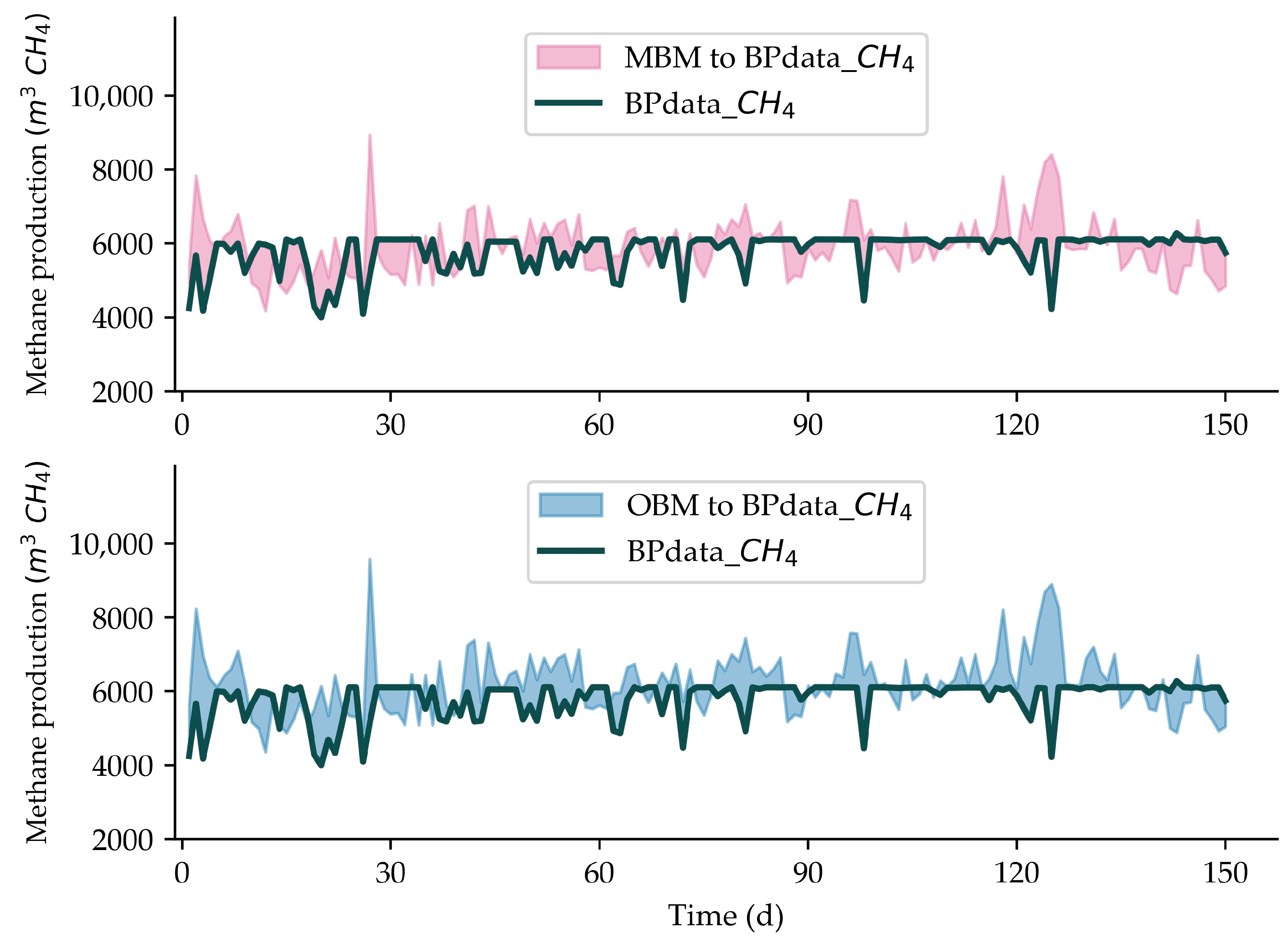
3.1. Model’s Validation

To evaluate the reliability of the proposed modifications to the simulation conditions, a validation study of 150 days was performed. For this purpose, the simulation results were compared with the data obtained from the full-scale biogas plant. Specifically, data from the biogas plant (BPdata) were compared against two simulations: the first BioModel simulation involved a decreasing working volume of the reactor over time (Modified_BioModel, MBM), while the second BioModel simulation maintained a constant volume throughout (Original_BioModel, OBM). Thus, the MBM simulation describes the real state of AD reactors of the plant, i.e., the continuous reduction of the working volume due to sedimentation of solid materials, starting at an initial volume of 4925 m³, whereas OBM simulates the reactor’s condition where no solids precipitation occurred and its initial volume remained constant at 7740 m³. Apart from the difference in volume, all other parameters (such as kinetic constants, yield coefficients, substrate composition, etc.) remained identical in both models. The steps followed to validate the model are included in a flowchart provided in the Supplementary Material.

To ensure the validity of the proposed modifications, particular attention was focused on the CH₄ production, given that the energy content of biogas exhibits a direct correlation with the concentration of CH₄ [49,50]. Thus, as CH₄ is responsible for the caloric value of biogas [51], it is directly linked to the profitability of the biogas plant and represents a reliable indicator directly related to the AD process.

Figure 3 shows the simulation outputs of MBM and OBM along with the estimated values of CH₄ production of the plant (BPdata_CH₄). Considering that the plant’s production was estimated based on daily electricity production, BPdata_CH₄ frequently exhibits a steady state around 6000 m³ d⁻¹, which represents the upper limit of electricity generation achievable by the CHP system. Given that the production rate of electricity cannot exceed the CHP capacity, the excess amount of CH_4, if produced, is stored under the membrane covering the reactor. However, since the BioModel does not consider the upper limit of 6000 m³ and the output depends on the reactor’s state and feedstock composition, in both simulation scenarios, it is evident that there is a tendency for overestimation of CH₄ production when compared to the BPdata_CH₄. Nevertheless, the model exhibited a commendable performance, frequently mirroring the fluctuations of the BPdata_CH₄.

For the comparative analysis of the two models, the average CH₄ production values from both MBM and OBM were employed considering the average BPdata_CH₄ throughout the entire period of study. The deviation observed in MBM was merely 1.97%, whereas OBM exhibited a larger variance of 7.33%.

For a better evaluation of the results, the 150-day period was divided into five sub-periods (periods 1–5), each of which corresponds to the average HRT of the plant (~30 days). The accuracy of the models’ simulations over each period was evaluated based on the PE and goodness of fit. The results are presented in

Table 2. Results of a 150-day study divided into five subperiods representing the average CH₄ production, PE and goodness of fit of the MBM and OBM simulations against the CH₄ production data of the plant.

Period	Duration	Average CH4 Production (m3)			PE (%)		Goodness of Fit
		MBM	BPdata	OBM	MBM to BPdata	OBM to BPdata	MBM to BPdata	OBM to BPdata
1	30 d	5630.10	5411.45	5899.57	4.04	9.02	0.96	0.90
2	30 d	5932.93	5757.57	6226.52	3.05	8.14	0.97	0.91
3	30 d	5923.13	5847.77	6236.80	1.29	6.65	0.98	0.93
4	30 d	6086.63	6013.02	6419.60	1.22	6.76	0.98	0.93
5	30 d	5999.49	5971.68	6344.19	0.47	6.24	0.99	0.93

, and as it appears, during the initial period (period 1), both MBM and OBM exhibit greater deviation from the plant’s data compared to the other periods. Specifically, MBM displays a discrepancy of 4.04% from BPdata_CH₄, while OBM displays a discrepancy of 9.02% from BPdata_CH₄. This initial variance could be attributed to the difficulty of the accurate simulation of startup periods. Potential delay in microbial growth, uncertainties about the reactor’s inoculum state and substrate used are some of the parameters that make the initial prediction of CH₄ production difficult when using stable kinetic models, such as the BioModel [52,53]. However, even at that starting period, MBM predictions were closer to BPdata_CH₄ when compared to the OBM predictions. In period 2, the performance of both models improved, with the MBM demonstrating greater responsiveness to BPdata_CH₄ than the OBM. Ιn subsequent periods (3 and 4), MBM outputs exhibited consistent enhancement and ultimately reached a difference of 0.47% from the BPdata_CH₄ (period 5), indicating a highly satisfactory agreement. Conversely, the OBM outputs in periods 3–5 maintained a consistent average deviation of 6.65% from the BPdata_CH₄.

It is important to acknowledge that the accuracy of the mechanistic models depends on the quality of the input data since the simulated CH₄ production is directly related to the substrate composition [54]. In full-scale biogas plants, such as the one in our study, the feedstock composition often undergoes frequent changes. Consequently, continuous analyses are usually not performed, which leads to reduced accuracy of the models. Despite these limitations associated with the study of full-scale biogas plants with varying feedstock, the MBM showed commendable CH₄ prediction results, significantly outperforming the OBM. Consequently, the MBM was further used in combination with Equation (8) to ascertain, from an economic point of view, the optimal time for the cleaning of the reactor, thus demonstrating its practical implications.

3.2. MBM & Developed T-Prediction Equation: A Combined Method as a Tool for the Prediction of Optimal Reactor Cleaning Period

After the model’s validation, the practical implementation of the MBM was explored in combination with the proposed equation (T-prediction, Equation (8)) as a tool for the determination of the optimal reactor cleaning period. As previously indicated, Equation (8) can be applied to any biogas plant for the prediction of the optimal cleaning period to achieve steady CH₄ production, given that the function of the increased cost due to the additional substrate (f(t)) is determined through the MBM. The method of finding f(t) is described below, and afterward, Equation (8) is used for the calculation of the cleaning period.

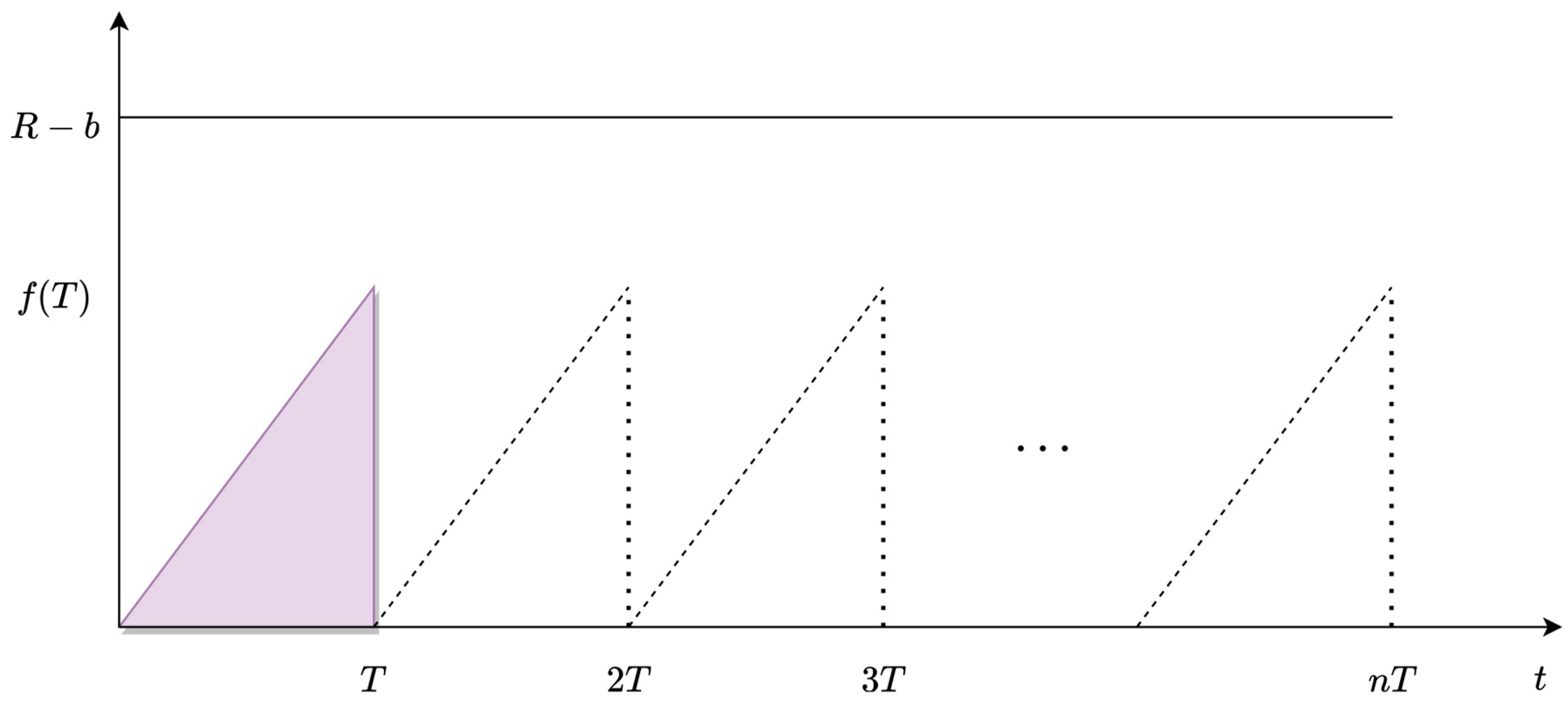
3.2.1. Discovering the Function of the Increased Cost through the MBM

Firstly, two simulations were considered: one regarding the operation of the plant where there is no reduction in the working volume (first simulation—steady CH₄ production), and one regarding the operation with a reduction of the working volume due to material precipitation (second simulation—working volume reduction). Real values of the biogas plant studied for the model’s validation were considered, i.e., initial reactor working volume of 7740 m³ (for both simulations), α value of 1.93 m³ d⁻¹ (second simulation only) and an initial OLR of 2.4 kgVS m⁻³_reactor d⁻¹, maintaining a constant flow throughout (in both simulations).

The simulation outputs are presented in Figure 4, where it is evident that the working volume reduction has a direct impact on CH₄ production, as the organic matter of the substrate remains for a shorter period in the reactor and part of it is not effectively converted to CH₄. During the first days, it appears that the CH₄ difference between the two curves increased rapidly, indicating an initial imbalance. However, in the following days, the decrease in CH₄ of the second simulation was more gradual, as expected.

For the determination of the required increase of substrate over time, an empirical approach was employed. Firstly, this included the calculation of the CH₄ difference between the two for each day. Subsequently, based on the decreasing CH₄ curve, the m³ CH₄/kgVS ratio was calculated. Finally, the difference in kgVS was estimated and expressed as the additional quantity of substrate (m³) that should be added so that both simulations have the same CH₄ production.

After the calculation of the additional amount of substrate, to ensure the validity of the proposed method, another simulation was performed. The third simulation (working volume reduction + added substrate) was carried out under the same initial conditions as the second one, including the same initial volume and the same reduction coefficient. However, in this case, the substrate volume was gradually increased, based on the aforementioned calculation. Simulations run for 365 days and their outputs are presented in Figure 5. The PE of the third simulation in relation to the target production (steady CH₄ production simulation) was approximately 0.13%, which was considered an acceptable level of variation. Nevertheless, to further improve the results, it is possible to repeat the procedure. Essentially, this involves recalculating the increase in the amount of substrate based on the curve resulting from the third simulation and making additional simulations, attempting to further minimize the deviation from the desired level of production.

After the final simulation, through Microsoft 365 Excel (Version 2310), a linear regression model was fitted to the increased substrate data to find the function describing their increase. The result was of the form y = ax + b, where the slope (a) was 0.0074, and the y-intercept (b) was 0.2967, with a Coefficient of Determination (R²) value of 0.998 (Figure 6). Since b is due to the generalization error of the model and has no physical meaning, it was not considered, and therefore, it can be assumed that the increase in the quantity of substrates approaches y = 0.0074x. By finding the slope of the increased substrate, it is possible to determine the form f(t), which is used in Equation (8). Hence, f(t) is the function of the increased substrate (slope a) multiplied by their acquisition cost (c), and its form is f(t) = (a·c)t.

3.2.2. Applying the T-Prediction Equation

After the determination of f(t), it was replaced by its specific form in Equation (8) and it turned out that the optimal cleaning period T is as follows:

$$\mathsf{{\rm T}}=\sqrt{\frac{2·\mathsf{{\rm K}}}{\mathrm{a}·\mathrm{c}}}$$

(9)

where:

K is the cost of cleaning the reactor and replacement of its membrane (if necessary).

a is the slope of the increased substrate curve.

c is the acquisition cost of the substrates.

As shown by Equation (9), the optimal reactor cleaning time depends only on the above three parameters (K, a, c). Given that K = 130,000 €, a = 0.0074 and c = 10 € m⁻³, the optimal cleaning time was calculated at 5.1 years, which is incidentally very close to the period in which the cleaning of the reactors of the studied plant was actually carried out. A general flowchart of all simulation stages is included in the Supplementary Material.

As it appears, the MBM, when combined with the T-prediction equation, can be a useful tool for predicting the optimal period for reactor cleanup with reasonable accuracy. Nevertheless, it should be noted that for modeling purposes, certain assumptions were made. Firstly, the development of the T-prediction equation was undertaken to mitigate the economic consequences of the working volume reduction as a result of the reduced degradation efficiency. This may lead to increased post-process CH₄ emissions, but it also represents a loss of renewable energy potential from biomass. Therefore, the option of increasing biomass input to counterbalance such accumulation problems is an economical approach to maintaining the full utilization of CHP capacity. Moreover, it should be clarified that the reactor’s working volume was considered to have a linear reduction over time with a constant α value. Hence, this assumption takes into consideration that since the biogas plant usually has the same suppliers, and the short-term variability is mainly seasonal, the substates used remain constant over a long period of time, as opposed to short-term periods where there is significant variation in substrate composition. Furthermore, it was assumed that no other instability was present in the AD process, i.e., high OLR, presence of inhibitors etc., and the reduced CH₄ is solely attributable to the working volume reduction. Therefore, further research may be conducted for the incorporation of the aforementioned parameters for the holistic evaluation of the working volume reduction.

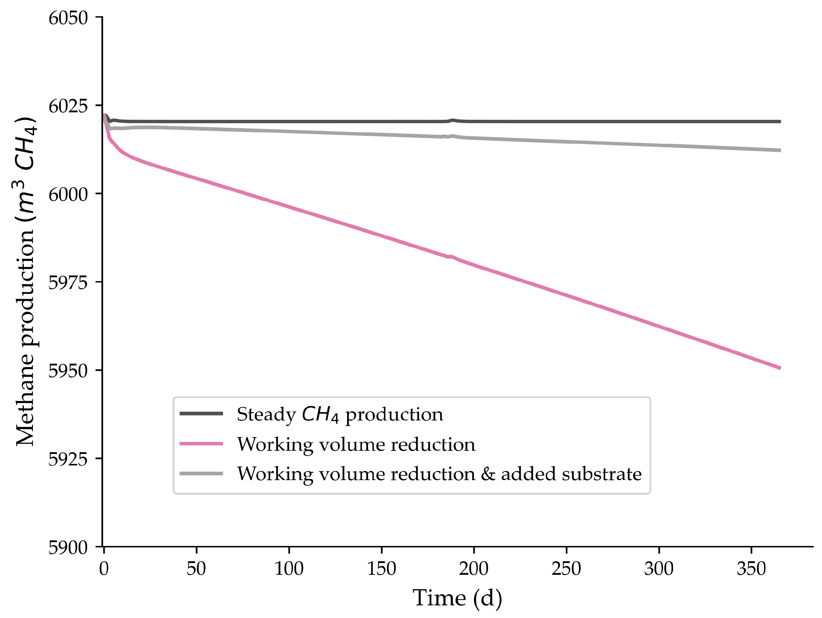
3.3. Significance of the Volume Reduction Coefficient (α)

The α value quantifies the rate at which the reactor volume decreases by accounting for the accumulation of inorganic material at the reactor’s bottom. Considering its inverse relation to the CH₄ production, various scenarios with different values of α were performed to demonstrate their impact on the optimal cleaning period of the reactor (T), which are illustrated in Figure 7.

In Figure 7, the different α values are expressed as a percentage of the working volume of the plant per year, ranging from 0, indicating no material accumulation, up to 23.8% of the working volume precipitating, which represents a substrate with a notably high concentration of (undesirable) heavy inorganics. It is evident that as the α increases, CH₄ production decreases significantly. A similar trend was also observed by Donoso-Bravo et al. [29]. The CH₄ difference of each scenario compared to the case with no volume reduction (α = 0), as well as the cleaning period calculated for each scenario, are presented in

Table 3. CH₄ difference results of various scenarios and their corresponding optimal cleaning times.

α (% of the Working Volume per Year)	CH4 % Difference over a Year	T (Years)
4.7%	0.59%	7.3
9.1% *	1.17% *	5.1 *
9.5%	1.23%	5.0
14.1%	1.93%	4.0
18.9%	2.72%	3.4
23.8%	3.65%	2.9

* Corresponds to the studied biogas plant scenario (mentioned in Section 3.2).

.

As expected, an increase in the α value leads to more frequent reactor cleanings to maintain maximum levels of CH₄ production and avoid economic losses for the plant. Nevertheless, it appears that there is no linear correlation between the working volume reduction and the optimal reactor cleaning period. Furthermore, the increase of α value is not inversely proportional to the CH₄ difference or the optimal reactor cleaning period.

4. Conclusions

The present study examined the working volume reduction due to inorganic material accumulation in AD reactors and the prediction of their optimal cleaning time. BioModel was used for the simulation of an existing biogas plant facing working volume reduction problems. For this reason, the simulation conditions were modified to incorporate a linear volume reduction (MBM). The results of the MBM and the OBM (without accounting for volume reduction) were compared against the estimated CH₄ production of the plant for a validation period of 150 days. During the starting period, both MBM and OBM exhibited significant deviations of 4.04% and 9.02%, respectively, from the plant’s data. However, the performance of the MBM was consistently improved, reaching a deviation of only 0.47% from the plant’s data, while the OBM deviated by 6.24%. After validation, an equation was developed for the calculation of the optimal reactor cleaning period with respect to the economic optimization of the plant’s profitability. The proposed equation was combined with the MBM, and the optimal cleaning period was calculated at 5.1 years, which was incidentally close to the time the plant actually carried out the cleaning of the reactors.

Furthermore, alternative scenarios were evaluated to determine the correlation between different α values and their corresponding optimal cleaning periods. Specifically, for ranging values of α = 4.7–23.8% of working volume per year, the optimal cleaning period interval corresponds to from 7.3 to 2.9 years. The results of this study demonstrated that the MBM, along with the proposed equation, can be used as a tool for the prediction of the optimal reactor cleaning period in a biogas plant. Further research may be conducted to investigate the working volume reduction in the presence of inhibitors or other AD instability and to explore how their synergistic effect affects the optimal reactor cleaning period.

References

1. Bumharter, C.; Bolonio, D.; Amez, I.; Martínez, M.J.G.; Ortega, M.F. New opportunities for the European Biogas industry: A review on current installation development, production potentials and yield improvements for manure and agricultural waste mixtures. J. Clean. Prod. 2023, 388, 135867. [Google Scholar] [CrossRef]
2. Kougias, P.G.; Angelidaki, I. Biogas and its opportunities—A review. Front. Environ. Sci. Eng. 2018, 12, 14. [Google Scholar] [CrossRef]
3. Kapoor, R.; Ghosh, P.; Tyagi, B.; Vijay, V.K.; Vijay, V.; Thakur, I.S.; Kamyab, H.; Nguyen, D.D.; Kumar, A. Advances in biogas valorization and utilization systems: A comprehensive review. J. Clean. Prod. 2020, 273, 123052. [Google Scholar] [CrossRef]
4. Nsair, A.; Cinar, S.O.; Alassali, A.; Abu Qdais, H.; Kuchta, K. Operational Parameters of Biogas Plants: A Review and Evaluation Study. Energies 2020, 13, 3761. [Google Scholar] [CrossRef]
5. Li, D.; Lee, I.; Kim, H. Application of the linearized ADM1 (LADM) to lab-scale anaerobic digestion system. J. Environ. Chem. Eng. 2021, 9, 105193. [Google Scholar] [CrossRef]
6. Kalamaras, S.D.; Vitoulis, G.; Christou, M.L.; Sfetsas, T.; Tziakas, S.; Fragos, V.; Samaras, P.; Kotsopoulos, T.A. The Effect of Ammonia Toxicity on Methane Production of a Full-Scale Biogas Plant—An Estimation Method. Energies 2021, 14, 5031. [Google Scholar] [CrossRef]
7. Roopnarain, A.; Rama, H.; Ndaba, B.; Bello-Akinosho, M.; Bamuza-Pemu, E.; Adeleke, R. Unravelling the anaerobic digestion ‘black box’: Biotechnological approaches for process optimization. Renew. Sustain. Energy Rev. 2021, 152, 111717. [Google Scholar] [CrossRef]
8. Wu, D.; Peng, X.; Li, L.; Yang, P.; Peng, Y.; Liu, H.; Wang, X. Commercial biogas plants: Review on operational parameters and guide for performance optimization. Fuel 2021, 303, 121282. [Google Scholar] [CrossRef]
9. Nielsen, H.B.; Angelidaki, I. Codigestion of manure and industrial organic waste at centralized biogas plants: Process imbalances and limitations. Water Sci. Technol. 2008, 58, 1521–1528. [Google Scholar] [CrossRef]
10. Eskicioglu, C.; Ghorbani, M. Effect of inoculum/substrate ratio on mesophilic anaerobic digestion of bioethanol plant whole stillage in batch mode. Process. Biochem. 2011, 46, 1682–1687. [Google Scholar] [CrossRef]
11. Cheng, Q.; Huang, W.; Xu, C.; Fan, G.; Yan, J.; Chai, B.; Zhang, Y.; Zhang, Y.; Zhang, S.; Song, G. Challenges of anaerobic digestion in China. Int. J. Environ. Sci. Technol. 2021, 18, 3685–3696. [Google Scholar] [CrossRef]
12. Fitamo, T.; Boldrin, A.; Dorini, G.; Boe, K.; Angelidaki, I.; Scheutz, C. Optimising the anaerobic co-digestion of urban organic waste using dynamic bioconversion mathematical modelling. Water Res. 2016, 106, 283–294. [Google Scholar] [CrossRef]
13. Biernacki, P.; Steinigeweg, S.; Borchert, A.; Uhlenhut, F.; Brehm, A. Application of Anaerobic Digestion Model No. 1 for describing an existing biogas power plant. Biomass Bioenergy 2013, 59, 441–447. [Google Scholar] [CrossRef]
14. Abilmazhinov, Y.; Shakerkhan, K.; Meshechkin, V.; Shayakhmetov, Y.; Nurgaliyev, N.; Suychinov, A. Mathematical Modeling for Evaluating the Sustainability of Biogas Generation through Anaerobic Digestion of Livestock Waste. Sustainability 2023, 15, 5707. [Google Scholar] [CrossRef]
15. Kegl, T.; Kralj, A.K. An enhanced anaerobic digestion BioModel calibrated by parameters optimization based on measured biogas plant data. Fuel 2022, 312, 122984. [Google Scholar] [CrossRef]
16. Fezzani, B.; Cheikh, R.B. Implementation of IWA anaerobic digestion model No. 1 (ADM1) for simulating the thermophilic anaerobic co-digestion of olive mill wastewater with olive mill solid waste in a semi-continuous tubular digester. Chem. Eng. J. 2008, 141, 75–88. [Google Scholar] [CrossRef]
17. Weinrich, S.; Nelles, M. Basics of Anaerobic Digestion: Biochemical Conversion and Process Modelling; Deutsches Biomasseforschungszentrum Gemeinnützige GmbH: Leipzig, Germany, 2021. [Google Scholar]
18. Enitan, A.M.; Adeyemo, J.; Swalaha, F.M.; Kumari, S.; Bux, F. Optimization of biogas generation using anaerobic digestion models and computational intelligence approaches. Rev. Chem. Eng. 2017, 33, 309–335. [Google Scholar] [CrossRef]
19. Satpathy, P.; Biernacki, P.; Cypionka, H.; Steinigeweg, S. Modelling anaerobic digestion in an industrial biogas digester: Application of lactate-including ADM1 model (Part II). J. Environ. Sci. Health Part A 2016, 51, 1226–1232. [Google Scholar] [CrossRef]
20. Ersahin, M.E. Modeling the dynamic performance of full-scale anaerobic primary sludge digester using Anaerobic Digestion Model No. 1 (ADM1). Bioprocess Biosyst. Eng. 2018, 41, 1539–1545. [Google Scholar] [CrossRef]
21. Emebu, S.; Pecha, J.; Janáčová, D. Review on anaerobic digestion models: Model classification & elaboration of process phenomena. Renew. Sustain. Energy Rev. 2022, 160, 112288. [Google Scholar] [CrossRef]
22. Walid, F.; El Fkihi, S.; Benbrahim, H.; Tagemouati, H. Modeling and Optimization of Anaerobic Digestion: A Review. E3S Web Conf. 2021, 229, 01022. [Google Scholar] [CrossRef]
23. Paladino, O. Data Driven Modelling and Control Strategies to Improve Biogas Quality and Production from High Solids Anaerobic Digestion: A Mini Review. Sustainability 2022, 14, 16467. [Google Scholar] [CrossRef]
24. Batstone, D.J.; Keller, J.; Angelidaki, I.; Kalyuzhnyi, S.V.; Pavlostathis, S.G.; Rozzi, A.; Sanders, W.T.M.; Siegrist, H.A.; Vavilin, V.A. The IWA Anaerobic Digestion Model No 1 (ADM1). Water Sci. Technol. 2002, 45, 65–73. [Google Scholar] [CrossRef]
25. Angelidaki, I.; Ellegaard, L.; Ahring, B.K. A mathematical model for dynamic simulation of anaerobic digestion of complex substrates: Focusing on ammonia inhibition. Biotechnol. Bioeng. 1993, 42, 159–166. [Google Scholar] [CrossRef]
26. Angelidaki, I.; Ellegaard, L.; Ahring, B.K. A comprehensive model of anaerobic bioconversion of complex substrates to biogas. Biotechnol. Bioeng. 1999, 63, 363–372. [Google Scholar] [CrossRef]
27. Kovalovszki, A.; Alvarado-Morales, M.; Fotidis, I.A.; Angelidaki, I. A systematic methodology to extend the applicability of a bioconversion model for the simulation of various co-digestion scenarios. Bioresour. Technol. 2017, 235, 157–166. [Google Scholar] [CrossRef]
28. Christou, M.; Vasileiadis, S.; Kalamaras, S.; Karpouzas, D.; Angelidaki, I.; Kotsopoulos, T. Ammonia-induced inhibition of manure-based continuous biomethanation process under different organic loading rates and associated microbial community dynamics. Bioresour. Technol. 2020, 320, 124323. [Google Scholar] [CrossRef]
29. Donoso-Bravo, A.; Sadino-Riquelme, M.C.; Valdebenito-Rolack, E.; Paulet, D.; Gómez, D.; Hansen, F. Comprehensive ADM1 Extensions to Tackle Some Operational and Metabolic Aspects in Anaerobic Digestion. Microorganisms 2022, 10, 948. [Google Scholar] [CrossRef]
30. Hartley, D.; Starr, S. Verification and Validation. In Estimating Impact: A Handbook of Computational Methods and Models for Anticipating Economic, Social, Political and Security Effects in International Interventions; Kott, A., Citrenbaum, G., Eds.; Springer US: Boston, MA, USA, 2010; pp. 311–336. [Google Scholar]
31. Donoso-Bravo, A.; Mailier, J.; Martin, C.; Rodríguez, J.; Aceves-Lara, C.A.; Wouwer, A.V. Model selection, identification and validation in anaerobic digestion: A review. Water Res. 2011, 45, 5347–5364. [Google Scholar] [CrossRef]
32. Yu, L.; Wensel, P.C.; Chen, J.M.A.S. Mathematical modeling in anaerobic digestion (AD). J. Bioremed. Biodeg. 2013, S4, 49–66. [Google Scholar] [CrossRef]
33. Panaro, D.; Mattei, M.; Esposito, G.; Steyer, J.; Capone, F.; Frunzo, L. A modelling and simulation study of anaerobic digestion in plug-flow reactors. Commun. Nonlinear Sci. Numer. Simul. 2021, 105, 106062. [Google Scholar] [CrossRef]
34. Wiedemann, L.; Conti, F.; Janus, T.; Sonnleitner, M.; Zörner, W.; Goldbrunner, M. Mixing in Biogas Digesters and Development of an Artificial Substrate for Laboratory-Scale Mixing Optimization. Chem. Eng. Technol. 2016, 40, 238–247. [Google Scholar] [CrossRef]
35. Kaparaju, P.; Buendia, I.; Ellegaard, L.; Angelidakia, I. Effects of mixing on methane production during thermophilic anaerobic digestion of manure: Lab-scale and pilot-scale studies. Bioresour. Technol. 2008, 99, 4919–4928. [Google Scholar] [CrossRef]
36. Hou, Y.; Xia, Q.; Yang, F.; Zhang, B.; Bian, Y.; Lei, Z.; Huang, W. Biogas circulation for improving the promotive effect of zero-valent iron on anaerobic digestion of swine manure. Bioresour. Technol. Rep. 2023, 21, 101319. [Google Scholar] [CrossRef]
37. Azizi, S.M.M.; Zakaria, B.S.; Haffiez, N.; Niknejad, P.; Dhar, B.R. A critical review of prospects and operational challenges of microaeration and iron dosing for in-situ biogas desulfurization. Bioresour. Technol. Rep. 2022, 20, 101265. [Google Scholar] [CrossRef]
38. Kegl, T. Consideration of biological and inorganic additives in upgraded anaerobic digestion BioModel. Bioresour. Technol. 2022, 355, 127252. [Google Scholar] [CrossRef]
39. Flores-Alsina, X.; Solon, K.; Mbamba, C.K.; Tait, S.; Gernaey, K.V.; Jeppsson, U.; Batstone, D.J. Modelling phosphorus (P), sulfur (S) and iron (Fe) interactions for dynamic simulations of anaerobic digestion processes. Water Res. 2016, 95, 370–382. [Google Scholar] [CrossRef]
40. Momoh, O.L.Y.; Anyata, B.U.; Saroj, D.P. Development of simplified anaerobic digestion models (SADM’s) for studying anaerobic biodegradability and kinetics of complex biomass. Biochem. Eng. J. 2013, 79, 84–93. [Google Scholar] [CrossRef]
41. Lovato, G.; Alvarado-Morales, M.; Kovalovszki, A.; Peprah, M.; Kougias, P.G.; Rodrigues, J.A.D.; Angelidaki, I. In-situ biogas upgrading process: Modeling and simulations aspects. Bioresour. Technol. 2017, 245, 332–341. [Google Scholar] [CrossRef]
42. Lovato, G.; Kovalovszki, A.; Alvarado-Morales, M.; Jéglot, A.T.A.; Rodrigues, J.A.D.; Angelidaki, I. Modelling bioaugmentation: Engineering intervention in anaerobic digestion. Renew. Energy 2021, 175, 1080–1087. [Google Scholar] [CrossRef]
43. Tsapekos, P.; Alvarado-Morales, M.; Kougias, P.G.; Konstantopoulos, K.; Angelidaki, I. Co-digestion of municipal waste biopulp with marine macroalgae focusing on sodium inhibition. Energy Convers. Manag. 2019, 180, 931–937. [Google Scholar] [CrossRef]
44. Tsapekos, P.; Kougias, P.; Alvarado-Morales, M.; Kovalovszki, A.; Corbière, M.; Angelidaki, I. Energy recovery from wastewater microalgae through anaerobic digestion process: Methane potential, continuous reactor operation and modelling aspects. Biochem. Eng. J. 2018, 139, 1–7. [Google Scholar] [CrossRef]
45. Razaviarani, V.; Buchanan, I.D. Calibration of the Anaerobic Digestion Model No. 1 (ADM1) for steady-state anaerobic co-digestion of municipal wastewater sludge with restaurant grease trap waste. Chem. Eng. J. 2015, 266, 91–99. [Google Scholar] [CrossRef]
46. Blumensaat, F.; Keller, J. Modelling of two-stage anaerobic digestion using the IWA Anaerobic Digestion Model No. 1 (ADM1). Water Res. 2005, 39, 171–183. [Google Scholar] [CrossRef]
47. Nabaterega, R.; Nazyab, B.; Eskicioglu, C. Modification and calibration of anaerobic digestion model 1 to simulate volatile fatty acids production during fermentation of municipal sludge. Biochem. Eng. J. 2023, 194, 108886. [Google Scholar] [CrossRef]
48. Sun, H.; Yang, Z.; Shi, G.; Arhin, S.G.; Papadakis, V.G.; Goula, M.A.; Zhou, L.; Zhang, Y.; Liu, G.; Wang, W. Methane production from acetate, formate and H2/CO2 under high ammonia level: Modified ADM1 simulation and microbial characterization. Sci. Total Environ. 2021, 783, 147581. [Google Scholar] [CrossRef]
49. Bond, T.; Templeton, M.R. History and future of domestic biogas plants in the developing world. Energy Sustain. Dev. 2011, 15, 347–354. [Google Scholar] [CrossRef]
50. Plugge, C.M. Biogas. Microb. Biotechnol. 2017, 10, 1128–1130. [Google Scholar] [CrossRef]
51. Rafiee, A.; Khalilpour, K.R.; Prest, J.; Skryabin, I. Biogas as an energy vector. Biomass Bioenergy 2020, 144, 105935. [Google Scholar] [CrossRef]
52. Wu, Y.; Kovalovszki, A.; Pan, J.; Lin, C.; Liu, H.; Duan, N.; Angelidaki, I. Early warning indicators for mesophilic anaerobic digestion of corn stalk: A combined experimental and simulation approach. Biotechnol. Biofuels 2019, 12, 106. [Google Scholar] [CrossRef]
53. Gaspari, M.; Alvarado-Morales, M.; Tsapekos, P.; Angelidaki, I.; Kougias, P. Simulating the performance of biogas reactors co-digesting ammonia and/or fatty acid rich substrates. Biochem. Eng. J. 2023, 190, 108741. [Google Scholar] [CrossRef]
54. Lindmark, J.; Thorin, E.; Bel Fdhila, R.; Dahlquist, E. Problems and Possibilities with the Implementation of Simulation and Modeling at a Biogas Plant. In Proceedings of the International Conference on Applied Energy ICAE 2012, Suzhou, China, 5–8 July 2012. [Google Scholar]
Figure 1. Daily feedstock fluctuation of the plant during the studied period of 150 days. The average flow rate of the plant was approximately 200 m3 d−1.
Sustainability 15 16157 g001
Figure 2. An illustration of the proposed framework described in Equation (6).
Sustainability 15 16157 g002
Figure 3. Simulation results of the Modified_BioModel (MBM) and the Original_ Biomodel (OBM) in comparison to the CH4 production (m3 d−1) of the biogas plant (BPdata_CH4—continuous line) for the studied period of 150 days. The shaded part illustrates their difference.
Sustainability 15 16157 g003
Figure 4. Simulation outputs of MBM in terms of stable CH4 production (first simulation) and working volume reduction (second simulation).
Sustainability 15 16157 g004
Figure 5. Simulation outputs of MBM in terms of stable CH4 production (first simulation), working volume reduction (second simulation) and working volume reduction with added substrate (third simulation) so that the decreasing CH4 curve (second simulation) approaches the first one as closely as possible.
Sustainability 15 16157 g005
Figure 6. Results of the empirical method for the calculation of the additional amount of substrate. The function in the box represents the obtained function describing their increase.
Sustainability 15 16157 g006
Figure 7. Different scenarios of α values, which are expressed as a percentage of the working volume of the plant per year.
Sustainability 15 16157 g007