An Artificial Physarum polycephalum Colony for the Electric Location-Routing Problem

Abstract

Electric vehicles invented for environmental sustainability are prone to adverse impacts on environmental sustainability due to the location and construction of their charging facilities. In this article, an artificial Physarum polycephalum colony is proposed to solve the novel challenging problem. First, the electric location-routing problem is established as a multi-objective network panning model with electric constraints to provide the optimal charging infrastructure layout, electric vehicle maintenance costs, and traffic conditions. The electric facility location problem and vehicle routing problem are integrated by integer programming, which considers the total distance, total time, total cost, total number of electric vehicles, and order fill rate. Second, an artificial Physarum polycephalum colony is introduced to solve the complex electric location-routing problem and includes the two basic operations of expansion and contraction. In the expansion operation, the optimal parent individuals will generate more offspring individuals, so as to expand the population size. In the contraction operation, only individuals with high fitness will be selected to survive through a merge sorting algorithm, resulting in a decrease in population size to the initial value. Through the iterative computing of the two main operations, the proposed artificial Physarum polycephalum colony can finally find the optimal solution to the objective function. Third, a benchmark test is designed for the electric location-routing problem by extracting the real road network from Tokyo, and the experimental results prove the effectiveness and applicability of this work.

1. Introduction

Electric vehicles (EVs) are widely popular worldwide due to their support for environmental sustainability, which can greatly reduce fossil fuel consumption and pollutant emissions. However, the construction and investment of charging facilities can also cause damage to environmental sustainability, so the electric location-routing problem (ELRP) is of great significance for promotion of EVs and environmental sustainability [1,2]. The ELRP is composed of two sub-problems: the electric facility location problem (EFLP) [3] and the electric vehicle (EV) routing problem (EVRP) [4]. The ELRP needs to determine the optimal location of electric depots and electric vehicle routes to fit the uncertain requirements of the customers and uncertain electric consumption to minimize costs [5] and energy consumption [6] and improve charging performance [7]. Both sub-problems belong to an NP-hard problem, so the ELRP is also an NP-hard problem and cannot be solved by precise algorithms.

In many studies, the two sub-problems are often studied separately to simplify the solution process [3,4]. However, a location problem solved without considering the routing problem will lead to an undesirable solution. In fact, these two sub-problems are closely related and inseparable. The solution to minimize the total cost of electric vehicle routing depends on the location of electric depots and routing networks [8,9,10]. Recently, researchers generally believe that the ELRP problem is a more complex task than a traditional location-routing problem (LRP). And the application of the ELRP will become increasingly widespread with the popularity of electric vehicles, such as charging station locations [2,11], battery swapping stations [12], smart cities [6], urban logistics [9,13], home health care [12], waste collection [14], electric trucks [7], electric aircraft [15], and electric buses [16].

To effectively solve the electric location-routing problem, many scholars have proposed various algorithms. A common objective is to reduce waiting times at charging stations with adaptive electric vehicle route planning [17]. This kind of method simplifies the ELRP into an orienteering problem (OP), the objective of which is to estimate a subset of nodes to be visited where the total objective function is maximized in a limited time duration. Hence, the ELRP can be considered as a combination of the knapsack problem and the traveling salesman problem (TSP) [18,19]. The TSP is an ancient LRP to maximize the total objective function of different routes limited by time duration, but the ELRP has to consider power consumption [6,9] and the layout of charging facilities while optimizing TSP, considering elements such as the charging station location [2,11], and battery swapping station location [12]. Therefore, the ELRP is an NP-hard problem where no polynomial-time algorithms can be used to effectively solve it, and the traditionally exact solution algorithms may be very time-consuming and not suitable for practical applications.

Recently, many heuristic or meta-heuristic methods were applied in the area, such as the genetic algorithm (GA) [5], artificial fish swarm algorithm (AFSA) [8], fuzzy logic (FL) [9], simulated annealing (SA) [12], particle swarm optimization (PSO) [18], deep reinforcement learning (DRL) [19,20], ant colony optimization (ACO) [21], machine learning (ML) and artificial neural networks (ANNs) [22], artificial bee colony (ABC) [23], and grey wolf optimization (GWO) [24]. These research works demonstrate that heuristic algorithms have great potential and can achieve good results in solving such NP-hard problems. However, heuristic algorithms also have some drawbacks, such as staying at the local optimal solution rather than the global optimal solution during the search process.

The above research work mainly focuses on optimizing and scheduling the operation of electric vehicles after the electric network is planned, and they rarely consider important factors such as charging infrastructure limitations, electric vehicle maintenance, and dynamic traffic conditions. If the electric network planning can be optimized before scheduling implementation, better solutions can be provided for the ELRP from the beginning, including better charging infrastructure layout and traffic conditions. The contributions of the paper are as follows.

First, the electric location-routing problem is modeled as a multi-objective function with electric consumption and constraints, which is built from the viewpoint of network panning before the EFLP and EVRP, rather than being split for a solution. In our solving mechanism, the primary issue is to select the optimal charging station location from a group of candidate nodes and generate a network to provide the optimal charging infrastructure layout, electric vehicle maintenance costs, and traffic conditions. The EFLP and EVRP are integrated in an ELRP, and evaluated by a multi-objective function considering the total distance, total time, total cost, total number of electric vehicles, and order fill rate.

Second, the multi-objective optimization function is solved by an artificial Physarum polycephalum colony algorithm. Inspired by the heuristic learning behavior of P. polycephalum [25] to efficiently search for nutrients and water in nature, a new artificial P. polycephalum colony (APPC) algorithm is designed to help us solve the complex ELRP. There are two main operations in the proposed APPC algorithm, including expansion and contraction. Different from traditional heuristic algorithms, the population size of the proposed APPC algorithm increases in expansion and decreases in contraction. In each iterative computation, the artificial P. polycephalum colony uses the multi-objective function of the ELRP as a fitness function and searches for more individuals. The optimal individuals may be well-saved through a merge sorting algorithm in each iteration, greatly improving the search performance of the algorithm.

Third, the Tokyo road network was adjusted for ELRP testing for the first time and our benchmark dataset comes from the real road network in Tokyo, which can demonstrate the practical application of our work. The experimental results verify the APPC algorithm can get better performance than other heuristic algorithms, and our solution has lower environmental damage and better environmental sustainability.

The remainder of this paper is organized as follows. In Section 2, the literature on the ELRP is reviewed. Section 3 presented the multi-objective function model of the ELRP. Details of the artificial P. polycephalum colony algorithm to solve the problem are presented in Section 4. In Section 5, numerical experiments are given to test the feasibility of the proposed APPC method. In the final section, the conclusions and future research directions are outlined.

2. Literature Review

Electric vehicles were born in response to environmental sustainability, but the location and development of charging facilities have also become the biggest problem faced by electric vehicles in use. The ELRP, as a new type of LRP problem, its solution directly affects the original intention of whether electric vehicles can achieve environmental sustainability [26,27]. Now, there are more and more research achievements in this area. The optimization of the ELRP is often multi-objective, where the electric consumption and charging heavily affects the optimization of facility location and distribution routes between the facilities and various nodes [4,5]. To reduce the difficulty of solving multi-objective ELRP problems, an effective method is to simplify the multi-objective optimization problem to a bi-objective optimization problem for solving. Ref. [28] reviewed LRP in terms of bi- and multi-objective optimization problems, and indicated that the decision-makers often encounter more than one objective, which are frequently conflicting. Due to the complexity and uncertainty of user behavior, the optimization work of the ELRP is very challenging. i.e., Ref. [29] provided robust locations and the sizing of electric vehicle battery swapping stations, considering users’ choice behaviors.

In the ELRP, lower electric consumption often helps to reduce transportation costs and carbon emissions, but this is often in conflict with high profits or order fill rate, which makes it difficult to solve this complex multi-objective problem [1,8,26]. To reduce the difficulty of solving, another approach is to decompose the complex ELRP problem into several sub-problems to be solved separately, i.e., the ELRP can be divided into the EFLP [29] and EVRP [30]. The EFLP is one of the sub-problems in the ELRP and is to decide the optimal location in the network, especially the electric charging stations [2,3,15,16,17] or the battery swapping stations [12,29]. In the EVRP, a single vehicle is required to achieve the maximum profit and minimum cost with constraints that the route duration is not more than a given threshold. However, the optimal solution to the EFLP may not be the optimal solution to the EVRP, due to factors such as the time window constraints [4,11,17]. Ref. [30] surveyed general variable neighborhood search algorithms in electric vehicle routing problems with time-dependent speeds and soft time windows. In the ELRP, the electric facility location and electric vehicle routes will together impact the total cost, but there is a diversification between them.

The complex ELRP can be seen as an orienteering problem, which is a combination optimization problem combining node selection, neighbor searching, the shortest Hamiltonian path, minimum cost, and maximizing the total score of the objective function [16,31,32]. Time windows and time-dependent scores are important methods for the ELRP, where a set of charging paths can be built to maximize the collected scores [4,11,17]. The score of visiting function is different depending on the time of charging. The location-inventory-routing problem (LIRP) is a common LRP that is based on a multi-stage demand forecasting model [33] and contains five parts of total logistics costs: the costs of trunk transportation and regional transportation, the fixed costs of distribution center construction, the inventory holding costs, shortage costs, and salvage, which are conflicting and are difficult to be optimized. This makes the issue of pickup and delivery of electric vehicles more complex [34].

To solve the complex ELRP, a lot of heuristic algorithms were employed recently. The heuristic algorithm is based on intuition or experience, which gives a feasible solution to each instance of the problem to be solved in an acceptable computing time and space. Besides the meta-heuristic algorithm [5,15,22,24], the swarm intelligence algorithm is very popular and can transmit and cooperate information through indirect communication [35]. Therefore, with the increase in the number of individuals, the increase in communication cost is small, and the heuristic algorithm has good scalability. The ability or behavior rules of each individual in a heuristic algorithm are very simple, so the realization of heuristic intelligence is relatively convenient and has the characteristics of simplicity. Examples include the genetic algorithm (GA) [5,36], artificial fish swarm algorithm (AFSA) [8], fuzzy logic (FL) [9,32], simulated annealing (SA) [12], particle swarm optimization (PSO) [18,37], deep reinforcement learning (DRL) [19,20,38], ant colony optimization (ACO) [21,39], machine learning (ML) and artificial neural networks (ANNs) [22,38,40], artificial bee colony (ABC) [23,41], grey wolf optimization (GWO) [24], artificial plant community (APC) [42], whale optimization algorithm(WOA) [43], and artificial slime mold (ASM) [13,44,45]. The heuristic algorithms can help us obtain a satisfactory feasible solution in a short time, but the deviation degree between the feasible solution and the optimal solution cannot be predicted. An overview of the related references is shown in

Table 1. Overview of related works.

Reference Number	Authors	Year	Objective	Benchmark Test
[1]	Wang C, et al.	2023	The total driving distance, the number of charging facilities, and the number of vehicles.	Modified classic TS-MOEA to solve the ELRP.
[2]	Hung YC, et al.	2022	To minimize the demand’s mean response time.	Designed an ELRP test extracted from Seattle in Washington state.
[8]	Liu Y, et al.	2020	Minimizing the costs for passengers and operators.	The transit network in an urban region of Beijing.
[9]	Ghobadi A, et al.	2022	The fixed cost of using EVs, the transportation cost, the penalty cost of time windows, and the cost of energy consumption.	Revised the Solomon benchmark to ELRP.
[11]	Wang Y, et al.	2022	The operating cost and the number of EVs.	Adjusted the EVCS-LRPTWRS in Chongqing City.
[13]	Cai Z, et al.	2022	The relative robustness, the betweenness robustness, the edge robustness, and the closeness robustness.	Modified the road network of Mexico City.
[15]	Kinene A, et al.	2023	To maximize regional connectivity and minimize the total investment costs for charging stations at airports.	The under-utilized regional airports in Sweden.
[16]	Liu XH, et al.	2023	To minimize the infrastructure investment, vehicle operating, battery electric bus purchase, recharging, and carbon emission costs.	The network of battery electric buses in Beijing.
[17]	Schoenberg S, et al.	2023	The driving, waiting, and charging time.	Extracted the road network of German Bundesnetzagentur from OpenStreetMap.
[21]	Manogaran G, et al.	2022	The first phase is to control delay and prevent EV failures, the second phase is to optimize the inputs of power and travel time.	A numerical example.
[25]	Tero A, et al.	2010	Network planning.	Tokyo railway system.
[29]	Zhang NW, et al.	2022	The EV users’ choice behavior, service levels, charging rate, and battery swapping service rate.	Real-world data from NYCTTLC are used to generate instances.
[30]	Matijevic L	2023	To minimize the total distance traveled by all vehicles and minimize the penalty for missing time windows for customers.	Modified a benchmark dataset presented in [31].
[32]	Velimirovic LZ, et al.	2023	The distance between the starting point, chargers, and final point, the amount of time spent at the charging station, and the attractiveness of the site.	A numerical example from the City of Niš.
[34]	Yilmaz Y, et al.	2022	To minimize the total distance traveled.	A numerical example.
[46]	Yang J, et al.	2015	To minimize total cost, including the construction cost of battery swap stations and EVs shipping cost.	Modified the classic VRP data sets to ELRP.
[47]	Amiri A, et al.	2023	To minimize the recharging cost, the initial recharging of the EVs, the acquisition cost, the labor cost, and the travel cost along the route.	Randomly generated several samples from Scarborough, Ontario.

.

As we can see from Table 1, the related works usually focus on optimizing and scheduling electric vehicles after the electric network planning, and they rarely consider important factors such as charging infrastructure limitations and layout, electric vehicle maintenance, and dynamic traffic conditions. Although it is better to optimize the network planning of the ELRP from the beginning, the benchmark tests for the ELRP are also rare. Due to the increasing attention paid to the ELRP in recent years [1,2,46,47], the main motivation of our work is to develop a more efficient solving mechanism for the ELRP. To the best of our knowledge, this is the first work to use an artificial P. polycephalum colony to address the ELRP from the viewpoint of network planning, and we also develop a benchmark test for the ELRP from the viewpoint of charging network planning.

3. Mathematical Formulation

To search for the optimal solution to the ELRP, two sub-problems of the EFLP and EVRP should be considered comprehensively in the objective function, rather than solved separately. In our solving mechanism, the primary issue is to select the optimal charging station location from a group of candidate nodes, and generate a network from the charging station to provide the optimal charging routes with the lowest energy consumption for other nodes. The objective function can be used as the fitness evaluation for an artificial P. polycephalum individual. When a better solution is found, the artificial P. polycephalum colony will use the new optimal solution to replace the past optimal one. An artificial P. polycephalum colony can continue the iterative computing procedure until the end conditions are matched. The optimal value of the objective function with the best charging station location and the optimal charging routes can be output as the optimal solution.

3.1. Symbol Definitions

This section gives the symbol definitions being used in the next sections, as shown in

Table 2. Symbol Definitions.

Symbol	Definition
N	A network node set
E	A network edge set
V	An electric vehicle set
n	A parameter for the total number of all nodes
pvk	A parameter for the power consumption coefficient of electric vehicle vk
Srkij	A parameter for the traveling speed of electric vehicle vk on edge Eij
Sckj	A parameter for the charging speed of electric vehicle vk on node Nj
Qvk	A parameter for the maximum transportation volume of electric vehicle vk
cc	A parameter for the unit construction cost
ch	A parameter for the unit holding cost
co	A parameter for the unit operating cost
Ite_max	A parameter for the maximum iterations
M	A parameter for the population size of APPC
ps	A parameter for the social-learning probability
pf	A parameter for the free-learning probability
eth	A parameter for the error threshold
Ni	A node
Ui	The user demand on node Ni
i	The node number
(xi, yi)	The coordinates of node Ni
Eij	The edge between nodes Ni and Nj
Dij	The distance between nodes Ni and Nj
D∑	The total distance of ELRP
di	The degree of node Ni
davg	The average degree of ELRP network
vk	An electric vehicle
V∑	The total number of electric vehicles
cvk	The electric capacity of electric vehicle vk
Qvki	The transportation volume of electric vehicle vk on node Ni
Pvk	The power consumption of electric vehicle vk
Trkij	The traveling time of electric vehicle vk between nodes Ni and Nj
Tckj	The charging time of electric vehicle vk on node Nj
T∑	The total time of the ELRP
Cc	The construction cost
Ch	The holding cost
Co	The operating cost
C∑	The total cost
O∑	The order fill rate
Ite	An iteration counter
m	The number of APPC individual
x	The variable of an artificial APPC individual
e	The solution error

.

For an ELRP, the node set of the whole network is N = {N_i|I = 1, 2,…,n}, where the coordinates of node N_i are (x_i, y_i). A node may be a depot, a charging station, or a user. The network edge set is E = {E_ij|i,j = 1,2,…,n }, and the geographical distance between nodes N_i and N_j is D_ij. The electric vehicle set is V = {v_k|k = 1, 2,…, V_∑}. Despite the difference between a depot and a charging station, the ELRP can be seen as a generated network of a candidate node. Similarly, despite the difference between the traveling distance or charging distance, the total distance can be used to measure the total operational cost of electric vehicles. Then, the total distance of the ELRP can be summed as D_∑. The value of degree on the node N_i is d_i, and the average degree of the ELRP network can be calculated as d_avg.

Then, the multi-objective network planning function can be used as the fitness function to help us select the optimal solution to the ELRP. Here, several important factors are used to evaluate the performance of the ELRP, such as the total distance, total time, total cost, total number of electric vehicles, and order fill rate. The solution to the ELRP can be defined as a graph G = (N, V), where the node set is N = {N_i|i = 1,2,…,n} and the network edge set is E = {E_ij|i,j = 1,2,…,n}. An electric vehicle v_k can pass through all nodes, and the traveling time T_rij is associated with the distance D_ij on each edge E_ij. Each node can be selected as a candidate charging station to generate a solution, and all electric vehicles start from the candidate to deliver goods to all users within the electric constraints. When electric energy is about to run out, electric vehicles must be charged. The charging time T_ckij is decided by the electric capacity c_vk, electric consumption P_vk, and charging speed S_ckij.

For the ELRP, the integer programming method can be used to define a solution variable x, which can be encoded as a series of charging stations and charging routes. In each iterative computation, the APPC will use a multi-objective function as to search for the optimal solutions, and the iteration counter Ite is used to count the number of iterative computations. The APPC uses social-learning probability p_s, self-learning probability p_f, and random-learning probability p_r to instruct the searching process. If the solution error e reaches the error threshold e_th, or the iteration counter Ite amounts to the maximum value Ite_max, then the evolutionary process will be stopped and the optimal solution will be output.

3.2. Building a Multi-Objective Function of the ELRP

A multi-objective function is proposed in the section to model the ELRP from the viewpoint of network planning. Generally, there are two major steps to solve the ELRP, namely the EFLP and the EVRP. In the EFLP, each node can be selected as a candidate charging station to connect all nodes. In the EVRP, a random search method is used to search for all vehicles to deliver the goods to all users where necessary charging routes are required. In the ELRP, an APPC algorithm is proposed to help us search for the optimal solutions both to the EFLP and to EVRP and provide the optimal charging infrastructure layout, electric vehicle maintenance costs, and traffic conditions. The multi-objective function should fully consider the optimal solution of the EFLP and EVRP from the beginning, where its purpose is to search for the optimal charging stations in the EFLP, and the charging stations have the optimal routes to connect all nodes in the EVRP. Based on the characteristics of the ELRP, the multi-objective function involves total distance, total time, total cost, total number of electric vehicles, and order fill rate.

Firstly, the total distance is used to connect all nodes by electric vehicles. The electric vehicles will select the depots or charging stations as the network center to construct different routes that connect all user nodes. The total distance can accurately evaluate charging infrastructure layout, electric vehicle maintenance costs, and traffic conditions from the viewpoint of space. The coordinates of nodes N_i and N_j are (x_i, y_i) and (x_j, y_j), then the geographical distance D_ij between nodes N_i and N_j can be calculated as follows.

$$D_{ij}=\sqrt{{(x_i-x_j)}^2+{(y_i-y_j)}^2}$$

(1)

In these routes, each electric vehicle should visit every node only once, and all electric vehicles can connect the user nodes within the electric constraints. According to the distance D_ij between two nodes N_i and N_j in Equation (1), the total distance D_∑ of the ELRP can be calculated as follows.

$$D_{\Sigma }={\displaystyle \sum _{i=1}^{i=n}{\displaystyle \sum _{j=1,j\ne i}^{j=n}{D}_{ij}}}$$

(2)

Secondly, the total time T_∑ is used to finish all deliveries and charges in a schedule and is the other important metric to accurately determine charging infrastructure layout, electric vehicle maintenance costs, and traffic conditions from the perspective of time. It includes traveling time and charging time. The traveling time T_rkij is calculated by the distance D_ij and the traveling speed S_rkij of electric vehicle v_k on the edge E_ij, where the distance D_ij on edge E_ij can be derived from Equation (1).

$$T_{rkij}=D_{ij}/S_{rkij}$$

(3)

The charging time T_ckj can be given by the electric capacity c_vk of electric vehicle v_k, electric consumption P_vk, and charging speed S_ckj on node N_j. According to the characteristics of electric vehicles, the electric consumption P_vk is decided by the power consumption coefficient p_vk of electric vehicle v_k, the traveling distance D_ij of electric vehicle v_k, and the square of the traveling speed S_rkij on edge E_ij. That is,

$$T_{ckj}=\frac{1}{S_{ckj}}(c_{vk}-P_{vk})=\frac{1}{S_{ckj}}(c_{vk}-{\displaystyle \sum _{i=1}^{i=n}{\displaystyle \sum _{j=1,j\ne i}^{j=n}{p}_{vk}{D}_{ij}{S}_{rkij}^2}})$$

(4)

Therefore, the longer the mileage and faster the traveling speed of electric vehicles, the greater their power consumption. Moreover, when the traveling speed doubles, the power consumption increases in a square order.

Based on the traveling time T_rkij in Equation (3) and the charging time T_ckj in Equation (4), the total time of the ELRP can be calculated as follows.

$$T_{\Sigma }={\displaystyle \sum _{i=1}^{i=n}{\displaystyle \sum _{j=1,j\ne i}^{j=n}(T_{rkij}+T_{ckj})}}$$

(5)

Thirdly, the total cost C_∑ includes the construction cost C_c, holding cost C_h, and operating cost C_o. It is another important indicator to accurately measure charging infrastructure layout, electric vehicle maintenance costs, and traffic conditions from the angle of costs. The construction cost C_c is the initial investment, including related expenses for facilities, equipment, and personnel, and is a one-time investment. The holding cost C_h varies linearly over time, meaning it continues to increase over time. The operating cost C_o mainly depends on the operating mileage of electric vehicles. The more vehicles there are and the longer the operating mileage, the higher the operating costs. That is,

$$C_{\Sigma }=C_c+C_h+C_o=c_{c}n+c_h{T}_{\Sigma }+c_o{D}_{\Sigma }$$

(6)

In the ELRP, there are n candidate charging stations at most, and each node has different topologies to visit all nodes, which generates different construction costs, holding costs, and operating costs. However, it is impossible to search for all solutions to an NP-hard problem. At the same time, different solutions can employ different total numbers of electric vehicles to deliver goods, which increases difficulties in solving the ELRP.

Fourth, the total number V_∑ of electric vehicles can be derived as follows. It investigates the efficiency of a network operating with fewer vehicles.

$${\displaystyle \sum _{i=1}^n{\displaystyle \sum _{k=1}^{V_{\Sigma }}(Q_{vki}})}\ge {\displaystyle \sum _{i=1}^n(U_i)}$$

(7)

The more electric vehicles there are, the higher the cost will be. The fewer electric vehicles there are, the lower the cost will be. However, the number V_∑ of electric vehicles is not simply as small as possible, as order fill rate O_∑ needs to be considered.

Fifthly, the order fill rate can be calculated based on the ratio of the transportation volume Q_vki of electric vehicle v_k on node N_i to the user demand on node i. It not only examines the node layout and edge connection cost of a network but also examines the weight of edge connections; that is, different edges have different transportation volumes.

$$O_{\Sigma }={\displaystyle \sum _{i=1}^n(\frac{1}{U_i}{\displaystyle \sum _{k=1}^{V_{\Sigma }}{Q}_{vki}})}$$

(8)

Therefore, based on the equations above, we can get the multi-objective network planning model for the ELRP, including the total distance D_∑ in Equation (2), total time T_∑ in Equation (5), total cost C_∑ in Equation (6), total number V_∑ of electric vehicles in Equation (7), and order fill rate O_∑ in Equation (8). The multi-objective function and constraints are as follows.

$$Obj\_fun=\left\{\min \right\{D_{\Sigma },T_{\Sigma },C_{\Sigma },V_{\Sigma }\},\max \{O_{\Sigma }\left\}\right\}$$

(9)

$$st1:p_{vk}{D}_{ij}{S}_{rkij}^2\le c_{vk}$$

(10)

$$st2:T_{rkij}\le \frac{c_{vk}}{p_{vk}{D}_{ij}{S}_{rkij}^2}$$

(11)

$$st3:T_{ckj}\le \frac{c_{vk}}{S_{ckj}^{}}$$

(12)

$$st4:{\displaystyle {\sum }_{i=1}^n{Q}_{vki}}\le Q_{vk}$$

(13)

$$st5:c_c>0,c_h>0,c_o>0$$

(14)

$$st6:\mathrm{if} (c_{vk}-P_{vk})\ge 0,\mathrm{then} S_{rkij}\ge 0;\mathrm{else} S_{rkij}=0$$

(15)

$$st7:p_{vk}>0,c_{vk}>0$$

(16)

$$st8:S_{rkij}>0,S_{ckj}>0$$

(17)

$$st9:Q_{vki}>0,Q_{vk}>0$$

(18)

As we can see from Equation (9), the objective function of the ELRP is composed of several conflicting objectives, where D_∑, T_∑, C_∑, and V_∑ take the minimum value, but O_∑ takes the maximum value.

Constraint 1 in Equation (10) indicates that the traveling distance D_ij and traveling speed S_rkij between the nodes N_i and N_j should not surpass the electric capacity c_vk.

Constraint 2 in Equation (11) indicates that the traveling time T_rkij of electric vehicle v_k between the nodes N_i and N_j is constrained by the electric capacity c_vk, traveling distance D_ij, and the cubic power of the traveling speed S_rkij.

Constraint 3 in Equation (12) indicates that the charging time T_ckj on the node N_j is constrained by the electric capacity c_vk and charging speed S_ckj of electric vehicle v_k. The maximum capacity c_vk of the electric vehicle battery is the maximum amount of electricity required for each charge on the node N_j.

Constraint 4 in Equation (13) indicates that the transportation volume Q_vki of electric vehicle v_k on all nodes should not surpass the maximum transportation volume Q_vk of electric vehicle v_k. Therefore, the maximum amount of cargo carried by an electric vehicle during each mission cannot exceed the vehicle’s own carrying capacity limit.

Constraint 5 in Equation (14) indicates that the unit construction cost c_c, unit holding cost c_h, and unit operating cost c_o are all positive numbers.

Constraint 6 in Equation (15) indicates that the traveling speed S_rkij is constrained by the remaining electric capacity (c_vk-P_vk) of electric vehicle v_k. If the remaining electric capacity is not enough, the electric vehicle will not be able to operate, namely S_rkij = 0. Therefore, electric vehicles should arrange charging routes as soon as possible before running out of battery and continue traveling after completing the charging process.

Constraint 7 in Equation (16) indicates that the power consumption coefficient p_vk of electric vehicle v_k and the electric capacity c_vk of electric vehicle v_k are all positive numbers and are decided by the type and characteristics of electric vehicle v_k.

Constraint 8 in Equation (17) indicates that the traveling speed S_rkij on the edge E_ij and the charging speed S_ckj on node N_j are all positive numbers and are decided by the type and characteristics of electric vehicles and charging stations.

Constraint 9 in Equation (18) indicates that the transportation volume Q_vki of electric vehicle v_k on node N_i and the maximum transportation volume Q_vk of electric vehicle v_k are all positive numbers.

The multi-objective function in Equation (9) and the constraints in Equations (10)–(18) comprehensively consider the EFLP of charging stations and the EVRP of electric vehicles. Both problems can be solved at the same time to get an optimal solution. The problem is so complicated that it is impossible to get all solutions within polynomial time. In the next section, a novel APPC algorithm is designed to help us solve this kind of complex multi-objective problem with many conflicting factors.

4. Algorithm Design of APPC

As we can see from Equations (9)–(18), the multi-objective function of the ELRP is more complex than a traditional location-routing problem, since there are a lot of constraints for electric capacity and charging requirements. Based on the merits and shortcomings of traditional algorithms, an artificial P. polycephalum colony algorithm is designed here which employs the heuristic learning mechanism of a natural P. polycephalum colony. The proposed APPC can collaboratively expand and contract to search for the optimal solution to the ELRP according to the fitness in Equations (9)–(18); that is, the artificial individuals with the highest fitness are the optimal solution.

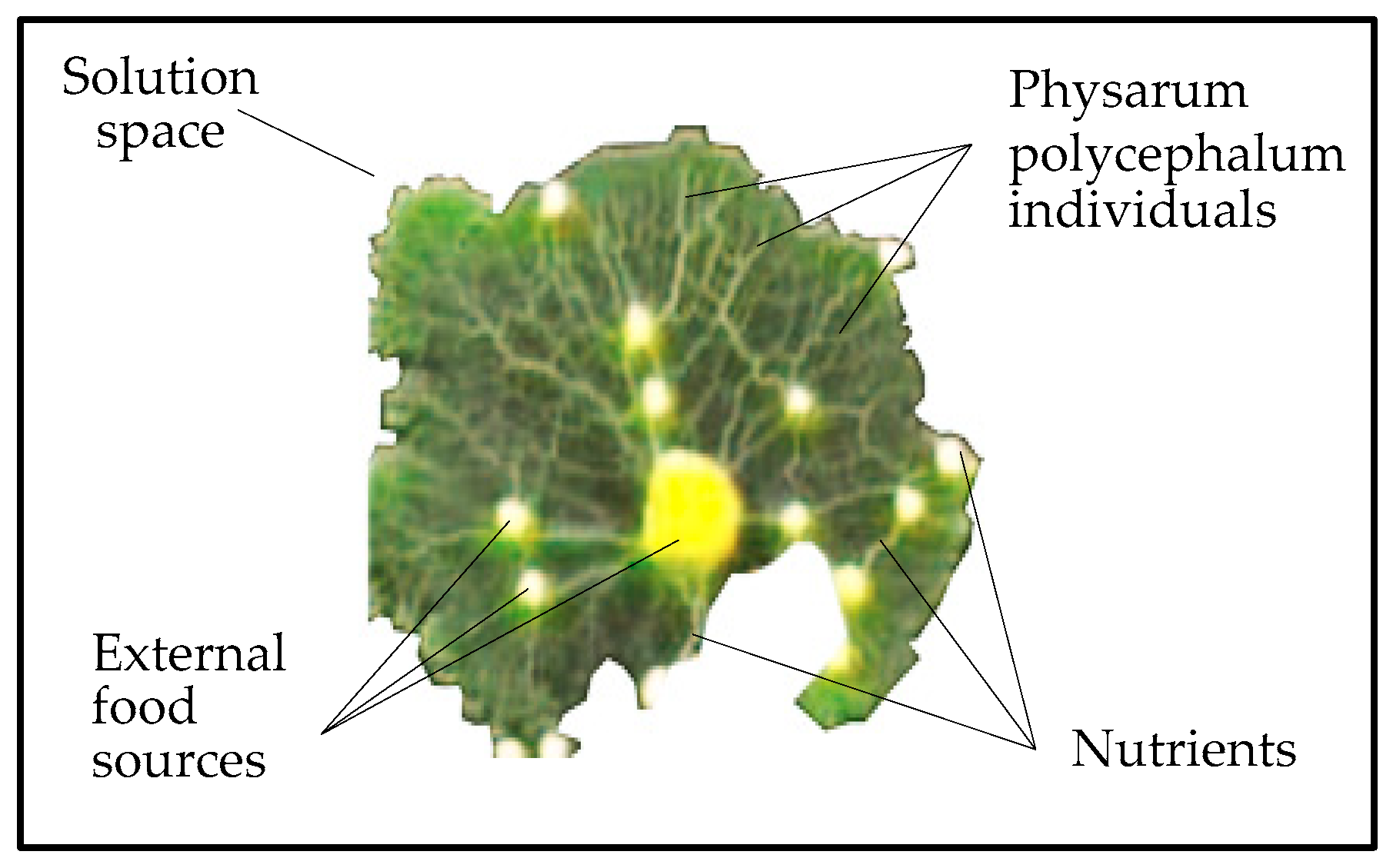
4.1. Artificial P. polycephalum Colony

Ref. [25] employed a natural P. polycephalum to design the Tokyo railway system and verified its strong parallel searching capability. After billions of years of evolution, the P. polycephalum colony in nature has an efficient mechanism to search for water and nutrients to survive [25]. The proposed heuristic learning mechanism is different from traditional heuristic algorithms and simulates the special behavior of P. polycephalum in the real world [25], and it utilizes variable population size to expand and contract. An artificial P. polycephalum colony is designed in Figure 1. In our APPC algorithm, there are four main components, i.e., the solution space, an artificial P. polycephalum colony, food sources, and a fitness function.

First, the solution space is the living area of an artificial P. polycephalum colony, meaning all possible solutions for the ELRP or other complex problems. An artificial P. polycephalum colony can expand and contract to search for feasible solutions in the solution space.

Second, several artificial P. polycephalum individuals constitute a P. polycephalum colony, and each individual is a filamentous organism. Different from traditional heuristic algorithms, the population size of the proposed artificial P. polycephalum colony will increase in expansion and decrease in contraction operations. All P. polycephalum individuals can learn from each other and share the solution knowledge. The learning behavior of an artificial P. polycephalum colony includes self-learning, social-learning, and free-learning.

Third, the food sources are the candidate nodes of the ELRP. They are randomly distributed in the solution space or organized according to a defined problem. The artificial P. polycephalum colony can randomly connect the food sources to absorb nutrients in its body. The artificial P. polycephalum individual connecting the food sources with the highest efficiency will survive; otherwise, it will disappear. An artificial P. polycephalum can search for the most efficient solutions to share the external food sources.

Fourth, the artificial P. polycephalum colony utilizes a fitness function to determine the living state of each individual. The artificial P. polycephalum colony will compare the fitness function in expansion and contraction operations. If an artificial P. polycephalum individual has a high fitness, it can be seen as a feasible solution. The fitness function can use the multi-objective function in Equations (9)–(18).

Based on the above four components, the artificial P. polycephalum colony employs two basic operations to implement the solution searching, i.e., expansion and contraction.

In the expansion operation, there are three kinds of learning methods, i.e., self-learning, social-learning, and free-learning. The population size will increase in the expansion operation, and there are three parts of individuals. After initialization, the artificial P. polycephalum colony has a population size of M, where each individual is randomly generated in the first initialization. In the expansion operation, the self-learning individuals with a population size of M keep the calculation results consistent with the previous iteration. However, a new part of social-learning individuals will be generated by learning from each other, and another new part of free-learning individuals will also be randomly generated. Now, the population size of the APPC in the expansion operation is greater than the original value M. This greatly increases the global searching capability of the APPC in the expansion operation.

In the contraction operation, the artificial P. polycephalum colony will select the best M of individuals, and then the population size of the APPC restores to the initial value M. The fitness comparison will instruct the APPC to compare and select the best individuals, and many individuals generated in the expansion operation will disappear after the contraction operation. The best individual is easy to preserve in our APPC algorithm, which is helpful in improving the local convergence capability. After a lot of expansion and contraction operations, the artificial P. polycephalum colony can find the optimal solutions to the ELRP.

The following sub-sections illustrate the whole solving process of our APPC algorithm, which includes four main stages, i.e., initialization, expansion, contraction, and end judgment. The first initialization stage is to set the main parameters and the objective function to be solved, where the original population of the APPC will be randomly generated in this stage. The second expansion stage is to expand the population of the artificial P. polycephalum colony for a heuristic search. The third contraction stage is to contract the population of the artificial P. polycephalum colony and generate the optimal solutions to the ELRP. Last, the end judgment stage is to judge whether the computational task is finished and to output the optimal solutions to the ELRP.

4.2. Step 1: Initialization

The initialization prepares the solving system of the APPC and problem parameters for the ELRP. There are four main parts in initialization, i.e., ELRP networks, electric vehicles, the artificial P. polycephalum colony, and the simulation system.

Substep 1-1: the initialization of the ELRP networks is to lay out the node and edge parameters of the ELRP. An ELRP network can be modeled as a graph G = (N, E) with a node set N and an edge set E. There is a total number n of nodes in the node set N, where a pair of position coordinates of a node $i$ is $(x_i,y_i)$. Then, there is an edge matrix $E={[E_{ij}]}_{n\times n}$ to connect the nodes, where the E_ij is the connection between the nodes i and j. The corresponding distance vector between any two nodes can be derived as $D=\left\{\right|E_{ij}\left|\right| i,j\in N\}$, where the distance between two nodes $(i,j)$ is determined by $\left|E_{ij}\right|=D_{ij}$. In the ELRP, the nodes may be a depot, a charging station, or a user. The solving task is to search for the optimal locations of charging stations for the EFLP and the optimal routes of electric vehicles for the EVRP at the same time. The objective function in Equation (2) can be used to calculate the location performance of charging stations.

Substep 1-2: the initialization of electric vehicles is to set the parameters of electric vehicles, including the user demand U_i on node i, the electric capacity c_vk of electric vehicle v_k, the maximum transportation volume Q_vk of electric vehicle v_k, the power consumption coefficient p_vk of electric vehicle v_k, the traveling speed S_rkij on the edge E_ij, the charging speed S_ckj on node N_j, the unit construction cost c_c, the unit holding cost c_h, and the unit operating cost c_o. The objective function in Equations (5)–(8) can be calculated to evaluate the route performance of electric vehicles.

Substep 1-3: the initialization of the APPC is to set the main parameters, including the population size M of the APPC, the social-learning possibility p_s, and the free-learning possibility p_f. Each artificial APPC individual can be randomly initialized as a binary string x, including the candidate charging station location and the candidate charging routes, so the corresponding fitness can be predefined as zero from the beginning. Similar to other heuristic algorithms, the solutions of our APPC algorithm have nothing to do with the initialization values.

Substep 1-4: the initialization of the simulation system should be preset. The multi-objective function to be solved should be defined here. The iteration counter is set as 0; all the objective values in Equations (9) and the solution error e should be cleared. The end judgment conditions should be predefined, i.e., the maximum iterations Ite_max, and the iteration error threshold e_th. These parameters will determine whether the iterative calculation of the APPC ends or continues.

4.3. Step 2: Expansion

In the expansion stage, an artificial P. polycephalum colony will generate more individuals to search for the optimal solutions, and the population size will increase to be more than the original value m. The expanded population {x} is composed of three parts, i.e., the self-learning colony {x_self}, the social-learning colony {x_social}, and the free-learning colony {x_free}.

$$\{x(Ite)\}=\{x_{self}(Ite-1),x_{social}(Ite),x_{free}(Ite)\}$$

(19)

Substep 2-1: the self-learning colony {x_self(Ite)} originates from the population {x_self(Ite-1)} generated in the previous iteration, i.e., the random colony generated during initialization in the first iteration, or the optimal colony generated during contraction operations in the previous iterations. Hence, this part of the colony is different between the first iteration and subsequent iterations. In the first iteration, this part of the self-learning colony is randomly generated, and the fitness of each individual may vary greatly, so the optimal solution cannot be determined. In the subsequent iterations, this part of the self-learning colony is inherited from the contraction operations in the last iteration calculation, so each individual has the optimal fitness in the previous iteration.

Subtep 2-2: the social-learning colony {x_social(Ite)} is produced by the self-learning colony through the social-learning mechanism. It simulates the heuristic behavior of a natural P. polycephalum colony and each pair of individuals will exchange some information with each other to generate a new generation of individuals. The social-learning mechanism employs the strategy of division and cooperation and helps to expand the search scope.

Substep 2-3: the free-learning colony {x_free(Ite)} is randomly produced and has nothing to do with the self-learning colony {x_self(Ite)} and the social-learning colony {x_social(Ite)}. Because of the random search, the free-learning increases the amount of different new solutions and helps to improve global search capability. The population size is determined by the possibility p_f.

Due to the self-learning population size of M, the social-learning population size of M, and the free-learning population size of p_fM, the total population size is (2 + p_f)M after the expansion operation. The increased population size endows the APPC algorithm with stronger global search capabilities than traditional heuristic algorithms, while also retaining strong local search capabilities. It can help the APPC algorithm solve the complex ELRP and similar challenging problems.

Based on the above merits, the pseudo-code of the expansion operation is presented here, as shown in Algorithm 1. The main parameters of the P. polycephalum colony include the total number n of nodes, the total number V_∑ of available vehicles, the population size of the artificial P. polycephalum colony is M, and the maximum number of iterations is Ite_max.

Algorithm 1: Expansion operation

1: Input: the ELRP networks, [(xi,yi)]n, D= [Dij]n×n

2: Input: electric vehicle parameters, Ui, cvk, vk, Qvk, pvk, Srkij, Sckj, cc, ch, co.

3: Input: APPC parameters, M, ps, pf.

4: Generate: random individuals {x}

5: Define: the fitness function in Equations (9)–(18)

6: Initialization: Ite_max, eth

7: For iteration counter Ite = 1: Ite_max

8:      For APPC individual m= 1:M

9:             For node number i = 1:n

10:                 To randomly select electric vehicle vk

11:                 Social-learning by ps

12:                 Free-learning by pf

13:              End for

14:       End for

15:       To update the APPC colony $\{x(Ite)\}=\{x_{self}(Ite-1),x_{social}(Ite),x_{free}(Ite)\}$

16:       To calculate the fitness according to Equations (9)–(18)

17: // Contraction operation

18: End for

As we can see from Algorithm 1, the expansion operation has a triple loop, so the time complexity can be depicted as $O(nMIte\_\max )$, and the space complexity is $O(nM)$. In the triple loop of expansion, the APPC uses total M individuals to search for total n nodes and total V_∑ available vehicles and selects the optimal solutions to the ELRP. The time and spatial performance are linearly correlated with the problem scale and main parameters, so the computational performance will not deteriorate sharply as the scale of the ELRP increases. The APPC expansion algorithm both has good search capabilities and good computational efficiency.

4.4. Step 3: Contraction

In the contraction stage, the artificial P. polycephalum colony will select the best M of individuals and the population size will decrease.

Substep 3-1: the APPC uses the multi-objective function in Equations (9)–(18) to evaluate the fitness of every individual, and most APPC individuals with low fitness will disappear.

Substep 3-2: Only the M total individuals with the highest fitness can survive after contraction, the other (1 + p_f)M of individuals with low fitness will disappear. The population size of the APPC increases from the original value M to (2 + p_f)M in expansion, but now the value again recovers to M. This well-simulates the heuristic behavior of a natural P. polycephalum colony and improves the local convergence performance to help us filter out the optimal solutions.

Similarly, the pseudo-code of the contraction operation is given here, as shown in Algorithm 2. Here, the merge sorting algorithm is employed to select the best individuals. The problem scale and main parameters of the P. polycephalum colony include total n nodes, total V_∑ available vehicles, the population size of the artificial P. polycephalum colony is M, and the maximum number of iterations is Ite_max.

Algorithm 2: Contraction operation

1: For iteration counter Ite = 1: Ite_max

2:       MergeSort(x, 1, M)

3:       To store the temporary optimal solution Temp_x = x(1)

4:       To store the temporary optimal fitness Temp_fitness = fitness(1)

5:       To calculate the iterative error e = |fitness (1)(Ite) − fitness(1)(Ite-1)|

6:       if e > eth

7:             select the best M of individuals

8:             return to the expansion algorithm

9:       else

10:             Exit

11: End for // Ite_max

12: output the optimal solution Temp_x

13: output the optimal fitness Temp_fitness

As we can see from Algorithm 2, the contraction algorithm has a twice loop and is embedded in the iteration loop. Due to the application of a merge sort algorithm, the average time complexity of the contraction algorithm can be given as $O(M{\log }_{2}M)$, where the best time performance and the worst time performance are also $O(M{\log }_{2}M)$. The space complexity is $O(M)$. Hence, the contraction operation of the APPC has high computational efficiency.

4.5. Step 4: End Judgment

Substep 4-1: the end conditions of the proposed approach can be judged by a predefined error threshold e_th, or the maximum of iterations Ite_max.

Substep 4-2: if the end conditions are not satisfied, the best M of individuals after the contraction operation will return to the expansion operation for the next iterative computation, and the operations of expansion and contraction will be repeated until the end conditions are met.

Substep 4-3: at last, the optimal solution and corresponding fitness will be output.

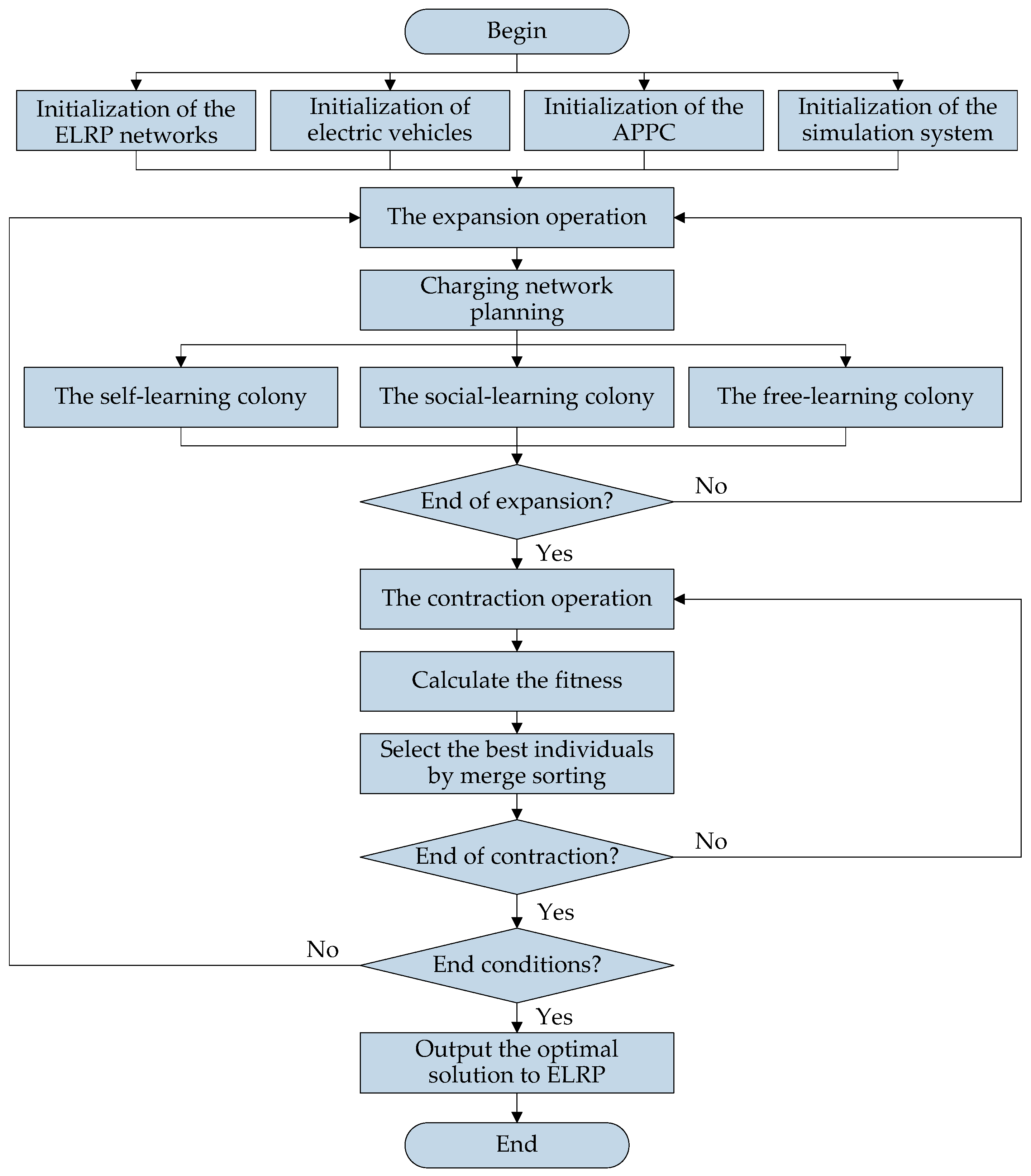
4.6. Algorithm Flow of APPC

In this section, the algorithm flow is summarized, as shown in Figure 2. The whole algorithm flow includes four main stages, namely initialization, expansion, contraction, and end judgment.

In the initialization stage, there are four main parts, i.e., ELRP networks, electric vehicles, the artificial P. polycephalum colony, and the system simulation parameters. The initial individuals of the APPC will be generated in this stage and the multi-objective function in Equations (9)–(18) will be defined here.

In the expansion stage, the P. polycephalum colony will search for the optimal solutions to the ELRP. The P. polycephalum colony will produce more individuals through self-learning, social-learning, and free-learning, so the population size will increase.

In the contraction stage, the P. polycephalum colony will evaluate the fitness of individuals and select the best ones for the next iterations. The individuals with low fitness will disappear and the population size will decrease to the original value.

After many iterations of expansion and contraction, it is possible to find the optimal solutions to the ELRP. A predefined error threshold e_th or the maximum of iterations Ite_max can be used for end justification before the optimal solutions are output.

4.7. Parameter Adjustment and Algorithm Improvement

The main parameters of the APPC include the population size M of the APPC, the social-learning possibility p_s, and the free-learning possibility p_f.

The population size M of the APPC decides the total number of feasible solutions in each iterative computation. The larger the M, the greater the individuals are generated in each iteration and the stronger the global search capability, but the slower the convergence rate and the greater the computational workload; on the contrary, the smaller the M, the fewer individuals are produced, the weaker the global search ability, but the faster the convergence rate and the lesser the computational workload.

The social-learning probability p_s determines the ratio of exchange parts where part of p_s comes from an individual and another part of 1-p_s comes from another individual. The larger the p_s, the more experience is kept from self-learning, the stronger the local search ability, and the faster the convergence rate; on the contrary, the smaller the p_s, the more experience is kept from social learning, the stronger the global search ability, but the slower its convergence rate. The social-learning of an artificial P. polycephalum colony increases the population size and improves global search performance.

The free-learning possibility p_f determines the population size of the freely exploring colony. The smaller the p_f, the more experience comes from self-learning and social-learning, the stronger the local search ability, and the faster the convergence rate; on the contrary, the larger the p_f, the more experience comes from free-learning and random search, the stronger the global search ability, but the slower its convergence rate.

The proposed APPC algorithm can also be improved by different strategies.

Alternative expansion strategies include three categories. The first is to adjust the population size after expansion, where a larger population size can help search for more solutions and a smaller population size can help provide fast convergence. The second is to adjust the social-learning mechanism, where each APPC individual can learn from several individuals through asexual reproduction, or each APPC individual can only learn from another individual to simplify the computing. The third is to adjust the encoding method of an APPC individual, such as binary encoding, integer encoding, and real encoding.

Alternative contraction strategies also include three categories. First, the population size after contraction can be adjusted, where a larger population size can help preserve more solutions and a smaller population size can help provide faster convergence ability. Second, the selection method of elite individuals can be adjusted to provide different convergence capabilities, such as selecting the only optimal individual, selecting a portion of the optimal individuals through different sorting algorithms, or random selection. Third, the fitness evaluation method can be adjusted, such as the analytic hierarchy process, multi-objective optimization, fuzzy evaluation, and advanced optimization methods.

5. Computational Results

5.1. Design of Benchmark Test

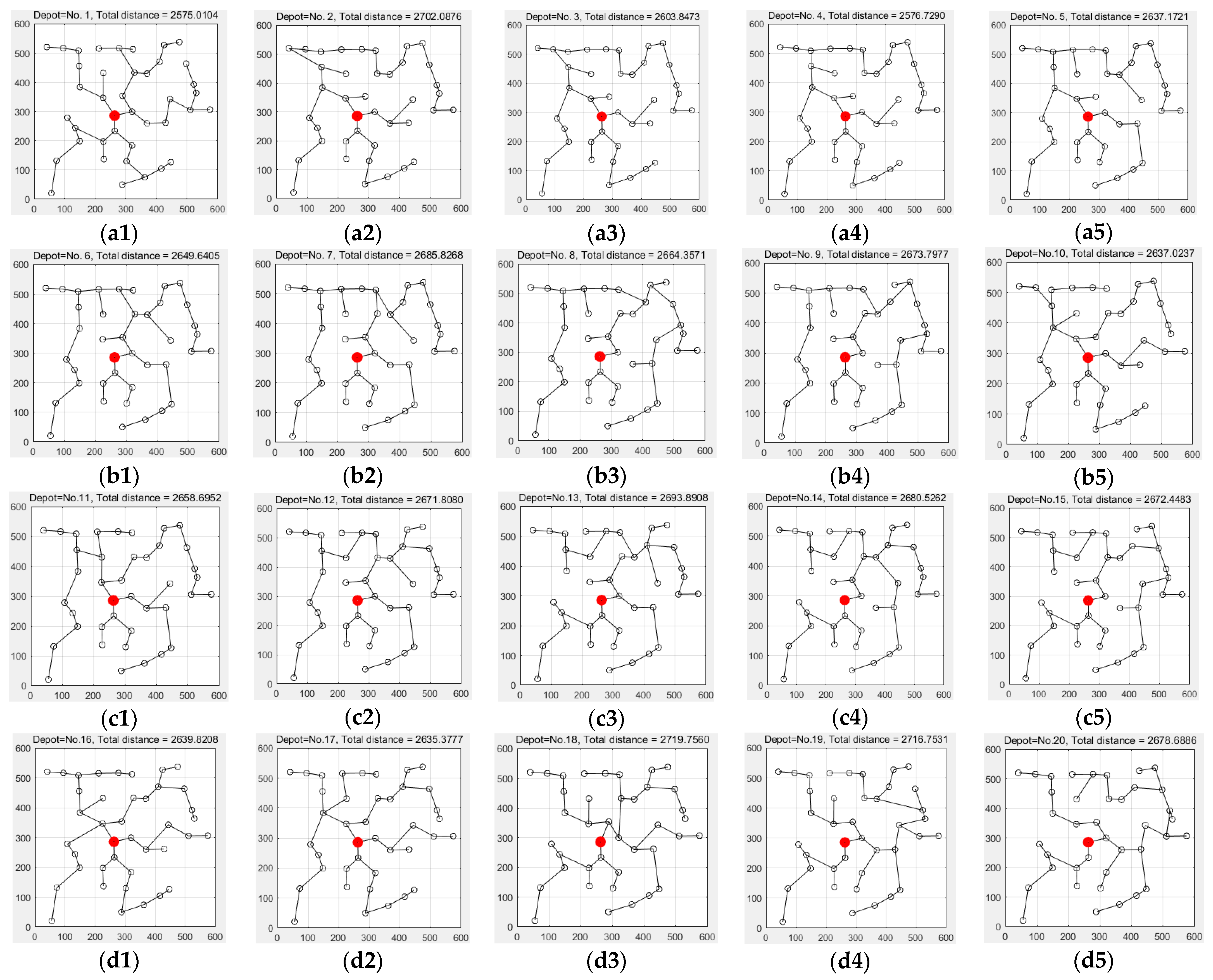
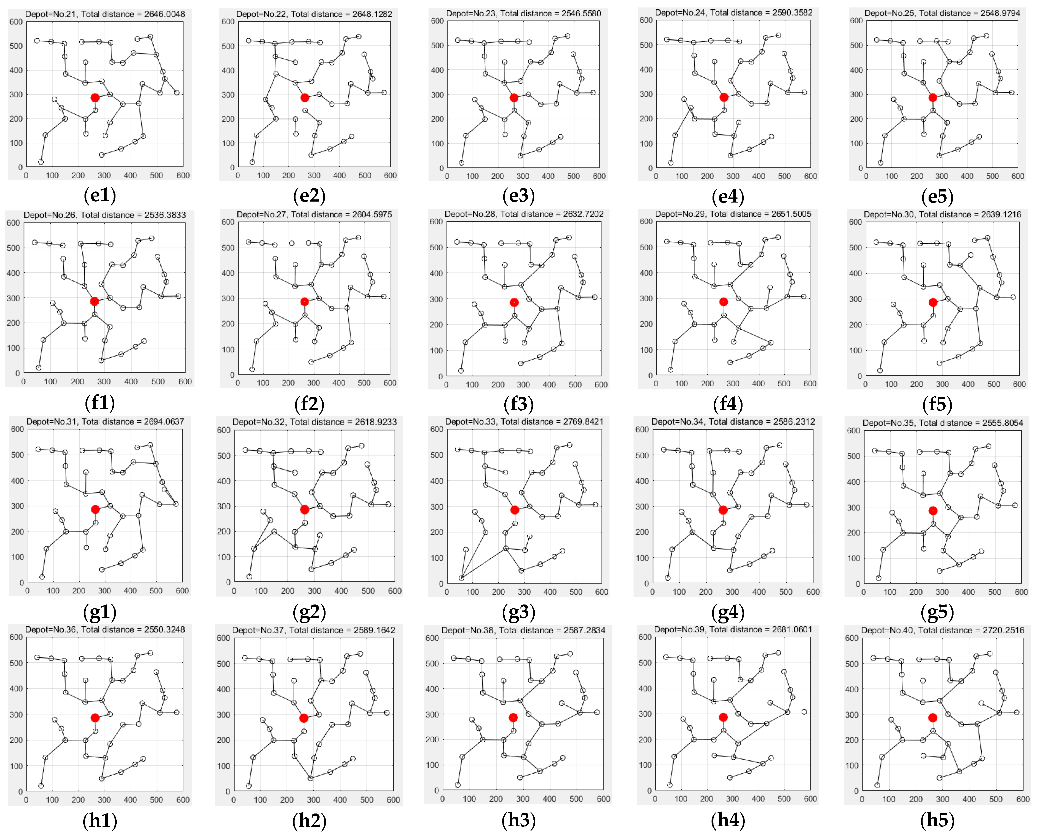
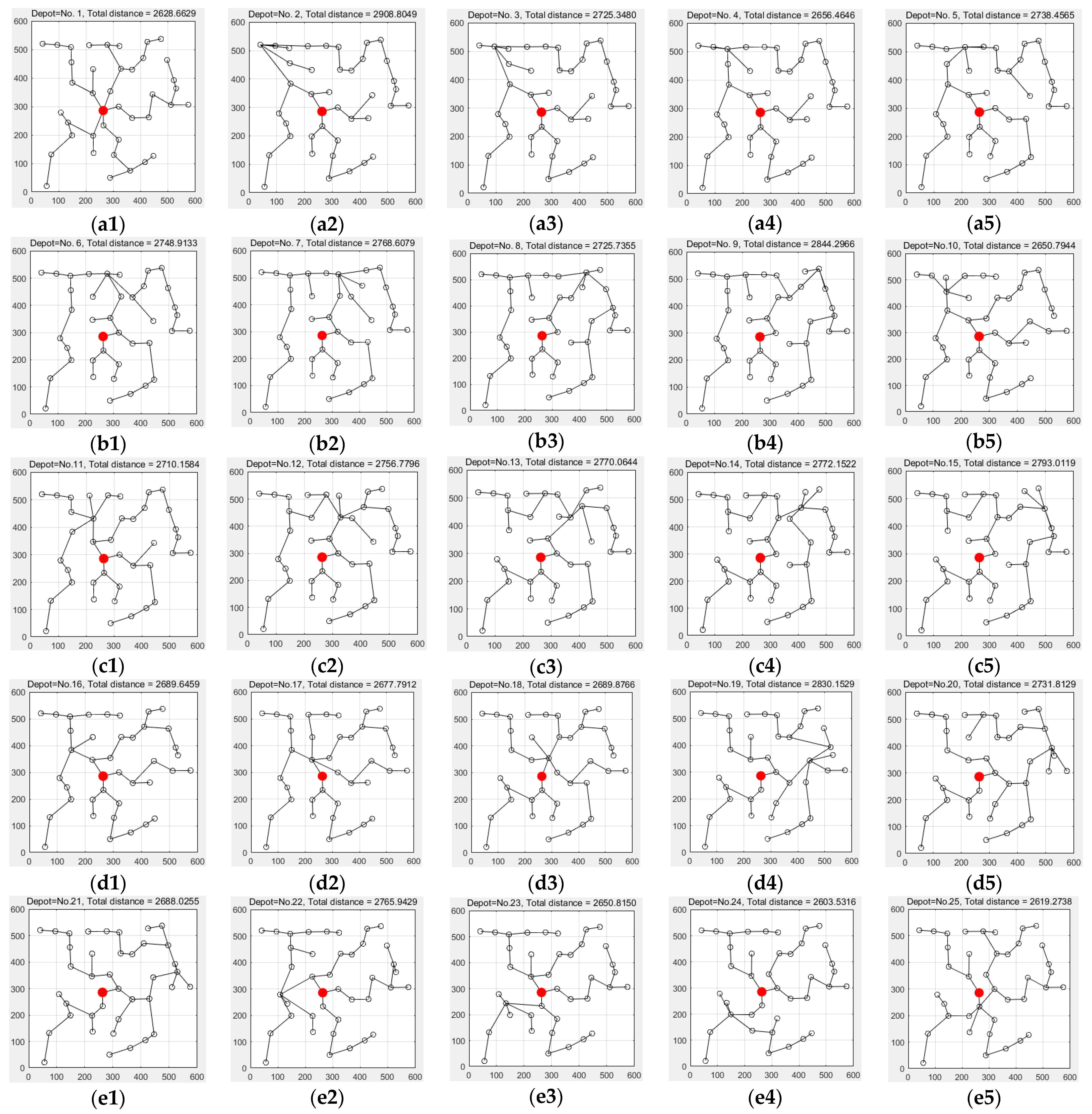
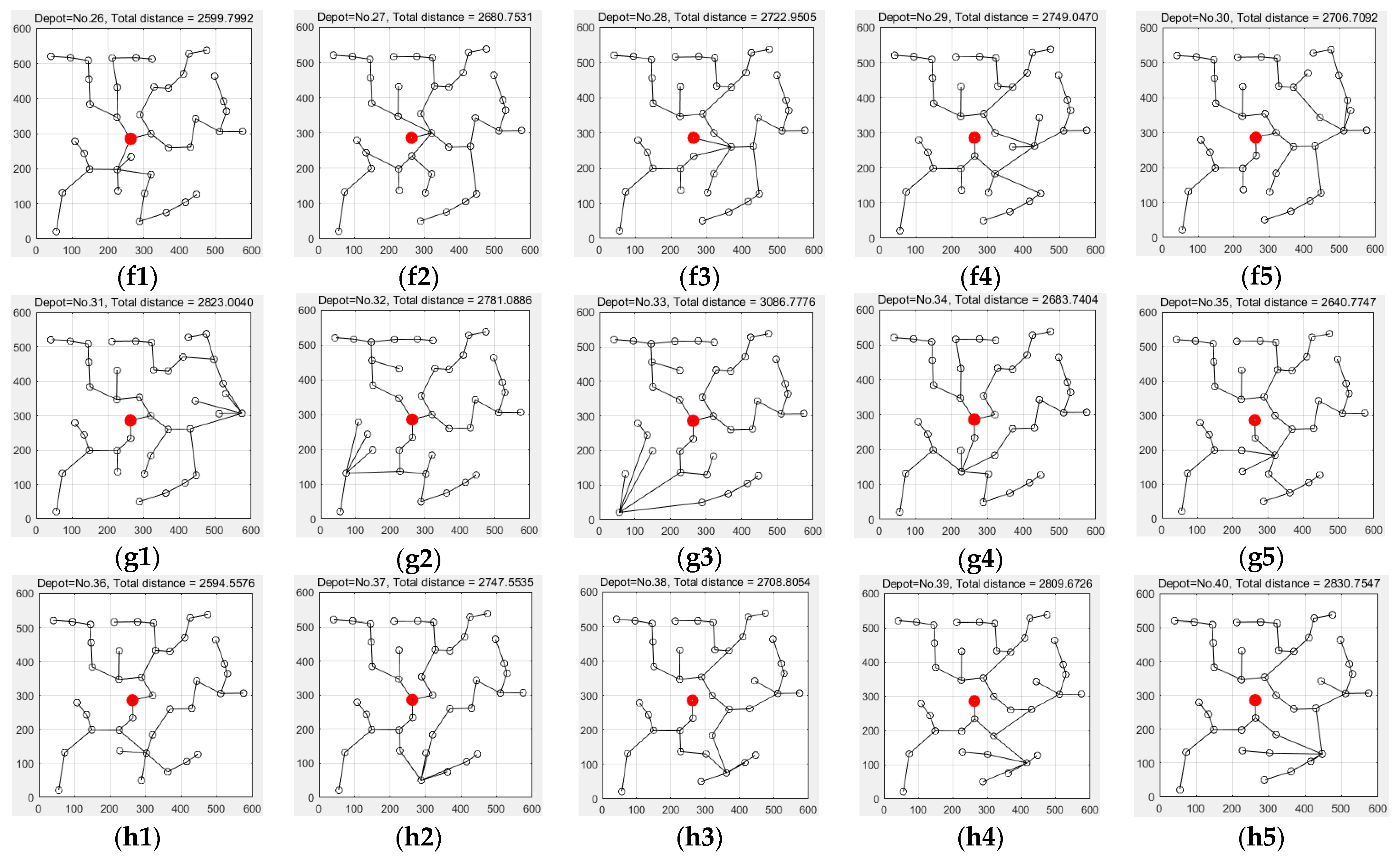
In this section, a benchmark test is especially designed to help us test the feasibility of our proposed APPC algorithm, and the proposed benchmark test is based on real data in Tokyo city [25], as shown in Figure 3. The Tokyo road system is one of the most famous road networks in the world, so using it for benchmark testing is more in line with our solving goals and has broad reference value. Tokyo has been promoting the use of electric vehicles for a long time, and making appropriate modifications to the classic LRP dataset can easily generate an ELRP benchmark test dataset. The wide availability of its data also facilitates the replication of test results by international peers. We have extended the Tokyo ELRP benchmark test set from the perspectives of scenario expansion, case studies, simulation modeling, and expertise, adding elements of electric vehicles and charging stations to make it a widely meaningful ELRP benchmark dataset. Japan is the world’s largest automobile exporter and has a deep technological foundation in fuel vehicles. With the accelerating trend of electrification, intelligence, and networking in the global automotive industry, how the Japanese automotive industry responds to the challenges and opportunities of new energy vehicles has become a noteworthy issue. Here, 40 nodes in total are selected for the experiment of the electric location-routing problem.

In our experiment, the 40 nodes in Tokyo are distributed in different areas, where node No.1 is Tokyo center, as shown in Figure 3. The ELPR of Tokyo is so complex that traditional algorithms cannot give all exact solutions in polynomial time. The proposed APPC algorithm is employed to solve it, and the main parameters include the population size M = 40, the social-learning probability p_s = 0.9, and the free-learning probability p_f = 0.1. The end conditions include the maximum iterations Ite_max = 200, and the error threshold e_th = 0.001. In each experiment, the APPC keeps these parameters unchanged. The experimental platform includes an AMD Ryzen 3 4300U with Radeon Graphics 2.70 GHz CPU, 8.00 GB RAM, a 64-bit Windows 10 operating system, and Matlab R2018a simulation software.

This ELRP case is challenging, and it is impossible to search for all feasible solutions. If any node is selected as a charging station, there are 40 possibilities. Each charging station uses a different number of branches to connect all nodes, with a maximum of 39 branches. In this section, the APPC was applied to solve the ELRP solutions and show three, four, and five branches of charging stations. Our artificial P. polycephalum colony algorithm spends little time in producing different optimal solutions by heuristic search. Our experimental results are in accordance with the real data of Tokyo City [25] in Figure 3. The fitness function is shown in Equations (9)–(18). In each experiment, the APPC generated an optimal solution to the ELRP according to the total distance, where each node can generate an optimal route connecting all nodes with different fitness. Since the total distance can determine the total time, total cost, and order fill rate, these experimental results may help us rank these solutions by their ELRP topologies and select the best solution to the ELRP.

5.2. Test Results

The solving process is based on our proposed APPC algorithm, where its solving steps are shown in Section 3, and the pseudo-code and flowchart are shown in Algorithms 1 and 2, and Figure 2. Figure 4 shows the simulated ELRP solutions with a parameter of three branches of charging stations, where the largest red node in the center of Figure 4 is marked as No.1 in the Tokyo road system, and the rest are other nodes in the system. Three electric vehicles in total can be employed, and the generated solutions can be used for the APPC to select the best solution to the ELRP. All the sub figures use three branches to connect all nodes and get the same average degree of 1.9500.

The proposed APPC can search the nodes around the charging station, where every node may be taken as the charging station, as shown in Figure 4(a1–i4). The APPC can form different topology connections around charging stations with different parameters. Although three electric vehicles are employed in total, the total length of the routing network increases from 2536.3833 in Figure 4(f1) to 2769.8421 in Figure 4(g3), while the average degree keeps stable at 1.9500. Therefore, the charging station of No.26 in Figure 3(f1) is the best one with a minimum total distance of 2536.3833, and the charging station of No.23 with a total distance of 2546.5580 in Figure 4(e3) is the second-best one. Additionally, node No.25 with a total distance of 2548.9794 in Figure 4(e5) is the third-best charging station, and node No.36 with a total distance of 2550.3248 in Figure 4(h1) is the fourth-best charging station. However, node No.1 with a total distance of 2575.0104 in Figure 4(a1) is the sixth-best solution in the location routing problem by its shortest route in the generated network, which is not consistent with our usual belief that node No.1 is the best center. In Figure 4, if three electric vehicles are employed, the six best solutions can be ranked by the total distance of their generated topologies as follows: No.26, No.23, No.25, No.36, No.35, and No.1.

More simulated ELRP solutions through parameter adjustment for the four branches of charging stations are shown in Figure 5(a1–i4), with the same average degree where the largest red node in the center of Figure 5 is marked as No.1 in the Tokyo road system. Compared with the results in Figure 4, the number of branches around the charging stations in Figure 5 increases from three to four, and more branches can help us find more efficient LRP solutions with the same average degree. Compared with the total distance in Figure 4, four vehicles in total can be employed, and the total distance in Figure 5 increases, which means that the total construction cost may increase, but the efficiency of operation may also increase.

In Figure 5, it is apparent that every node can be selected to form a route with different topologies each time. Although four electric vehicles are employed in total, the total length of the generated route increases from 2553.6100 to 2897.9641, but the average degree is kept at 1.9500. Comparing the total distance in Figure 4, the best route is the generated topology from node No.36 with a total distance of 2553.6100 in Figure 5(h1), and the second-best route is the generated topology of No.26 with a total distance of 2556.3468 in Figure 5(f1). Combining the results in Figure 4, where node No.26 is the best node for the charging station, its generated topology is still one of the best two routes among all solutions in Figure 5. In addition, nodes No.23 in Figure 5(e3) and No. 25 in Figure 5(e5) are still important nodes in the ELRP because of their third and fourth shortest total distance and equal average degree. In addition, node No.1 with a total distance of 2585.5459 in Figure 5(a1) is the fifth-best solution in the location routing problem. In Figure 5, if four electric vehicles are employed, the six best solutions can be ranked by the total distance of their generated topologies as follows: No.36, No.26, No.23, No.25, No.1, and No.35.

After that, more ELRP solutions through parameter modification for the five branches of charging stations are simulated and shown in Figure 6(a1–i4), with the same average degree, where the largest red node in the center of Figure 6 is marked as No.1 in the Tokyo road system. Compared to the results in Figure 6 and Figure 7, the number of branches around the charging stations in Figure 6 increases from three, to four, to five, and more branches further increase the total distance. Five electric vehicles in total can be employed, and Figure 6 can help us find more efficient ELRP solutions with the same average degree. Although five electric vehicles are employed in total, the best route is still the generated topology from node No.36 with a total distance of 2594.5576 in Figure 6(h1), and the second-best route is still the generated topology of No.26 with a total distance of 2599.7992 in Figure 6(f1). In addition, node No.1 with a total distance of 2628.6629 in Figure 6(a1) is the fifth-best solution in the location routing problem. Compared to the total distances in Figure 4 and Figure 5, the total distance and total cost in Figure 6 further increase, but the average degree and robustness may also increase. In Figure 6, if five electric vehicles are employed, the six best solutions can be ranked by the total distance of their generated topologies as follows: No.36, No.26, No.24, No.25, No.1, and No.35.

Summing up the results in Figure 4, Figure 5 and Figure 6, the proposed APPC is verified to be able to search for optimal solutions to the ELRP and select the best locations for charging stations to connect all the nodes in Tokyo city after the continuous evolution and heuristic learning. To our surprise, after many tests, the traditional central node is not the optimal solution to the ELRP, and some neighboring candidate nodes are more suitable for being the network center of the optimal solution to the ELRP because of their better routing network. According to the ELRP solutions with different total distances, the APPC can help us rank these nodes by the multi-objective function in Equations (9)–(18).

5.3. Sensitivity Analysis

This section employs sensitivity analysis to investigate the performance of the proposed method in solving the ELRP. Sensitivity analysis can help us excavate the primary decision factors and the main parameters of the ELRP to determine the impacts of potential changes in the solving process.

First, sensitivity analysis is used to examine the parameter relationship between the total distance and total number of vehicles. Figure 7 shows the total distances of different solutions to corresponding charging stations with branch numbers three, four, and five. The total distance can be computed by Equation (2), where shorter total distance means shorter total time, lower total cost, and higher order fill rate. Comparing the results in Figure 4, Figure 5 and Figure 6, the proposed APPC can accurately generate a lot of feasible solutions and rank them to select the best one and has advantages in solving speed and accuracy. Furthermore, the APPC can help us produce more solutions besides the results in Figure 4, Figure 5 and Figure 6. More branches may result in higher total costs and more electric vehicles for the ELRP solutions, but fewer electric vehicles is also an important goal in objective Equations (9)–(18).

As we can see from Figure 7, the best solution of the ELRP is node No.26 with three vehicles and a total distance of 2536.3833, as shown in Figure 4(f1). Next, the second-best solution of LRP is node No.36 with four vehicles and a total distance of 2553.6100 in Figure 5(h1) or with five vehicles and a total distance of 2594.5576 in Figure 6(h1). Although node No.1 is a traditional urban center, it is not suitable to be the optimal solution to the ELRP in these three cases. In general, the total cost of three-branch ELRP solutions is smaller than those of four-branch and five-branch feasible solutions. Additionally, in the ELRP, none of the edge nodes are suitable for the optimal solution of the ELRP problem, such as No.2, No.9, No.31, No.33, and No.40. To set charging stations on edge nodes will greatly increase the total distance, total time, total cost, and reduce the order fill rate.

Second, sensitivity analysis is applied to check the stability of the optimal solutions in different charging routes, as shown in

Table 3. Sensitivity analysis of the optimal solutions in different charging routes.

Number of Branches	1st Optimal Solution	2nd Optimal Solution	3rd Optimal Solution	4th Optimal Solution	5th Optimal Solution	6th Optimal Solution
3	No.26 (2536.3833)	No.23 (2546.5580)	No.25 (2548.9794)	No.36 (2550.3248)	No.35 (2555.8054)	No.1 (2575.0104)
4	No.36 (2553.6100)	No.26 (2556.3468)	No.23 (2572.7760)	No.25 (2576.8416)	No.1 (2585.5459))	No.35 (2598.4972)
5	No.36 (2594.5576)	No.26 (2599.7992)	No.24 (2603.5316)	No.25 (2619.2738)	No.1 (2628.6629)	No.35 (2640.7747)

. Among all three scenarios, node No.26 can be selected as an optimal solution representation used in the proposed heuristic algorithm. For the number of branches = 3, Figure 4(f1) with a total distance of 2536.3833 is the optimal solution to the ELRP. If the number of branches = 4, Figure 4(f1) can be modified to be Figure 5(f1) with a total distance of 2556.3468 as the optimal solution to the ELRP. Furthermore, if the number of branches = 5, Figure 5(f1) can be modified to be Figure 6(f1) with a total distance of 2599.7992 as the optimal solution to the ELRP. After this modification, the solution representation in our proposed heuristic algorithm can adapt to different scenarios of the ELRP.

Third, sensitivity analysis is employed to check the parameter relationship between the multi-objective function and the dynamic traffic conditions, as shown in

Table 4. Sensitivity analysis of the multi-objective function in dynamic traffic conditions.

Traffic Jam	Total Distance D∑	Total Time T∑	Total Cost C∑	Total EVs V∑	Order Fill Rate O∑
0%	2536.3833	58.3077	3855.3026	3.0000	0.9428
10%	2607.4020	67.3486	4113.8546	3.0000	0.9107
20%	2716.9129	79.7469	4458.1020	3.0000	0.8689
30%	2863.6262	96.6129	4900.8896	3.0000	0.8185

. When the probability of traffic jams increases from 0% to 30%, and the total number of vehicles remains unchanged at three, the total distance, total time, and total cost all increase significantly, but the order full rate decreases greatly. Compared to the most severe traffic conditions (30%) and noncongested traffic conditions (0%), the total cost increased by 27.12% and the order fill rate decreased by 13.19%.

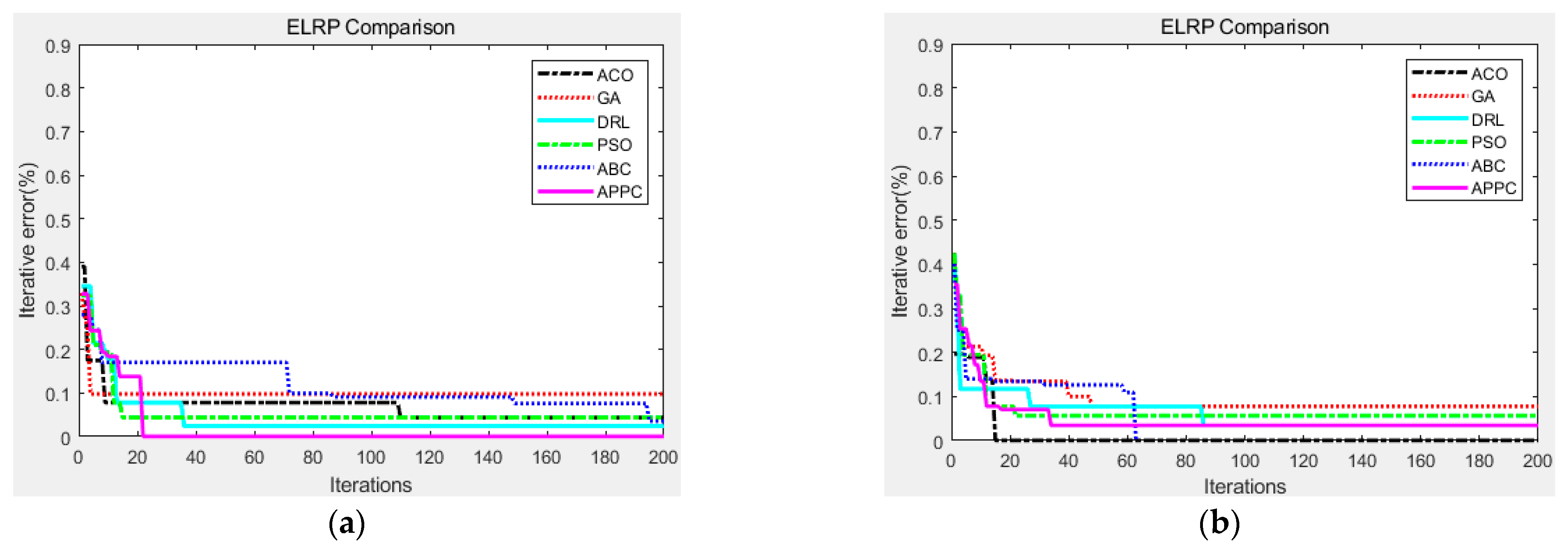
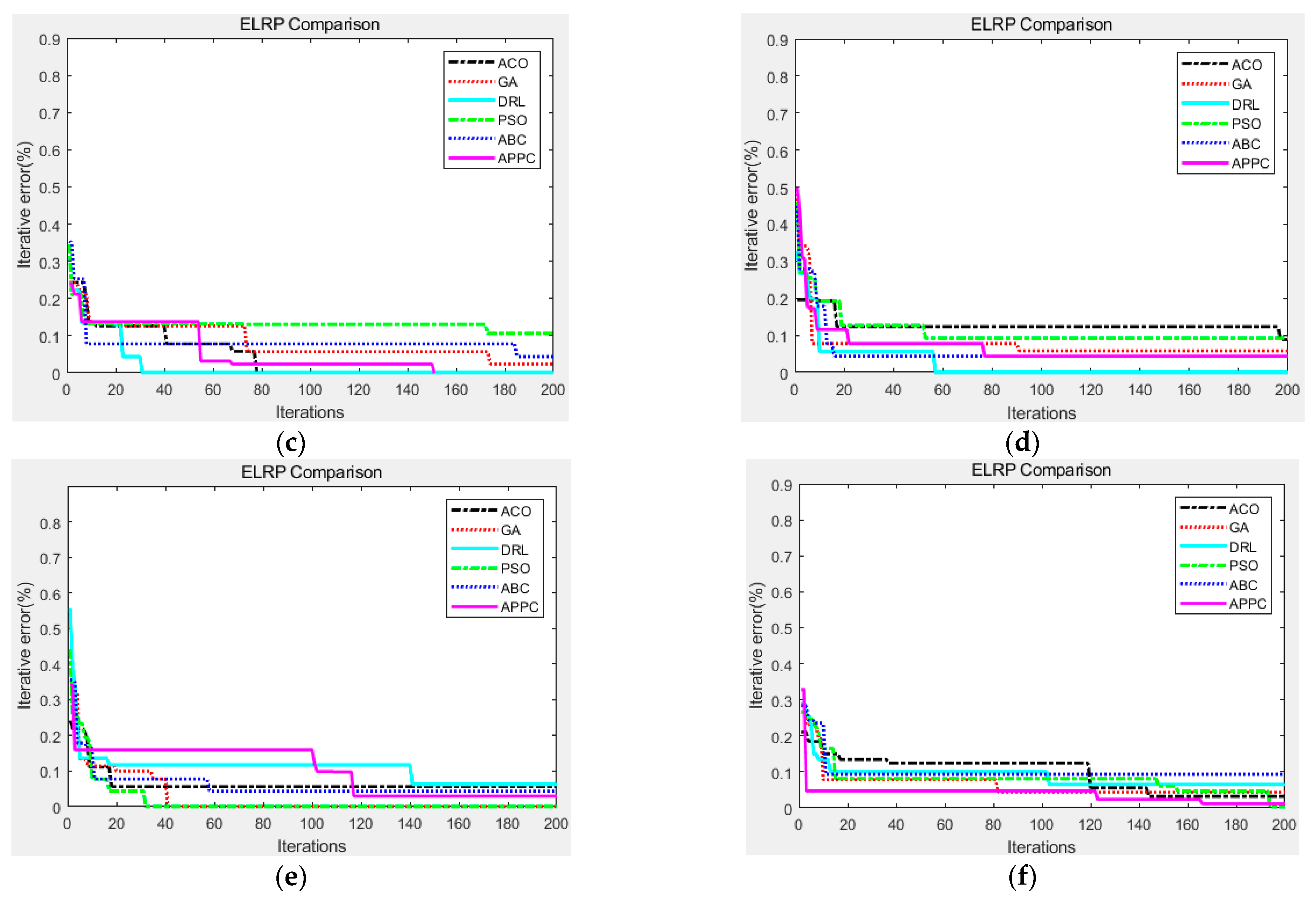
5.4. Comparison of State-of-the-Art Algorithms

Furthermore, the proposed APPC algorithm and other state-of-the-art algorithms are employed to solve the multi-objective function in Equations (9)–(18) for performance comparison, as shown in Figure 8. The reference state-of-the-art algorithms include the genetic algorithm (GA) [5,36], particle swarm optimization (PSO) [18,37], deep reinforcement learning (DRL) [19,20,38], ant colony optimization (ACO) [21,39], and artificial bee colony (ABC) [23,41]. For the GA [5,36], the population size was set to M = 40, the chromosome length was Lind = 20, the crossover probability was px = 0.7, and the mutation probability was pm = 0.01. For the PSO [18,37], the population size was set to M = 40, the location limitation was 0.5, the speed limitation was [−0.5, 0.5], the self-learning factor was c1 = 1.0, and the social learning factor was c2 = 1.0. The parameters of the DRL [19,20,38] were a convolutional neural network with six convolution cores, six input channels (c_in = 6), and six output channels (c_out = 6). The learning rate of the offset item was twice that of the weight. The extension edge was set to 0, the weight was initialized to Gaussian, and the value of the constant offset item was 0. The parameters of the ACO [21,39] included a population size M = 40 ants, a pheromone importance of 1.0, a heuristic factor importance of 5.0, and a pheromone volatilization factor of 0.1. For the ABC [23,41], it was set so the population size is M = 40, the searching limit parameter is 100, and the neighborhood size is NI = 10.

It is assumed that all algorithms employ the same population size M and iteration steps Ite_max to solve the same ELRP with n nodes. Figure 8 presents the convergence curves of different algorithms with the error threshold e_th = 0.001. Even compared with traditional AI algorithms, the proposed artificial P. polycephalum colony algorithm will help us search for the optimal solutions to the ELRP and often needs a shorter solving period.

As we can see from Figure 8, the proposed APPC can be applied in solving the ELRP as with the other heuristic algorithms. It also verifies that the ELRP is an NP-hard problem and traditional algorithms cannot get all accurate solutions in a polynomial time. Compared with the traditional heuristic algorithms, the proposed APPC algorithm is less likely to fall into the local optimal solution region prematurely and can get consistent experimental results with high accuracy. The solving mechanism of the proposed APPC method is different from traditional AI algorithms, but it is less susceptible to changes in the scale of the problem when the total number of ELRP nodes increases from 40 to 240. It is worth mentioning that each algorithm does not necessarily have to have the same number of iterations, since each algorithm has a different iteration computational complexity. Here, we just prove the convergence of each method, and we have no intention of belittling other algorithms.

For further analysis, the comparison of average iterative errors on multi-objective function is shown in

Table 5. Comparison of average iterative errors on multi-objective function.

Multi-Objective	GA [5,36]	PSO [18,37]	DRL [19,20,38]	ACO [21,39]	ABC [23,41]	Proposed APPC
Total distance D∑	7.215 × 10−4	5.571 × 10−4	4.962 × 10−4	6.519 × 10−4	7.066 × 10−4	5.804 × 10−4
Total time T∑	5.732 × 10−4	7.194 × 10−4	5.607 × 10−4	6.144 × 10−4	5.417 × 10−4	6.081 × 10−4
Total cost C∑	6.846 × 10−4	6.905 × 10−4	6.051 × 10−4	7.320 × 10−4	5.935 × 10−4	4.752 × 10−4
Total EVs V∑	7.573 × 10−4	7.609 × 10−4	7.180 × 10−4	5.382 × 10−4	6.490 × 10−4	5.029 × 10−4
Order fill rate O∑	5.967 × 10−4	5.728 × 10−4	6.236 × 10−4	7.038 × 10−4	7.473 × 10−4	4.694 × 10−4
Computing time (ms)	548	733	1557	562	619	571

, where the objectives include total distance D_∑, total time T_∑, total cost C_∑, total vehicle V_∑, order fill rate O_∑, and computing time (ms). The top five metrics can be calculated by Equations (9)–(18), and the computing time is calculated based on the start and end times of each algorithm. The error threshold is set as e_th = 0.001, and the computing time depends on the time to reach the iteration error, not the number of iterations. After 30 tests, we obtained the average values of these metrics, and the best results in each metric are highlighted in bold formatting.

As we can see from Table 5, our proposed APPC algorithm achieved three optimal values out of five indicators, such as the bold values in Table 5, but did not achieve a maximum value. All the heuristic algorithms get similar average iterative errors on the main objectives, including total distance D_∑, total time T_∑, total cost C_∑, total vehicle V_∑, and order fill rate O_∑. For all heuristic intelligence algorithms, the time performance is linearly related to the population size M and the scale n of the ELRP. However, there is no swarm learning mechanism in SA [12], and its time performance is decided by the ELRP scale n and the number Ite_max of iterations. However, the time performance of the DRL [19,20,38] and ANNs [22,38] is related to the scale n of the ELRP, the population size M of the convolution cores, the number c_in of input channels, and the number c_out of output channels. To get similar computational errors, the DRL [19,20,38] and ANNs [22,38] will consume more computing time.

5.5. Insight for Engineering Applications

For engineering applications, more factors should be considered, such as scenario expansion, case studies, expert experience, and actual modeling. According to Figure 3, Figure 4, Figure 5, Figure 6, Figure 7 and Figure 8 and Table 2, Table 3, Table 4 and Table 5, the proposed APPC algorithm has some advantages in solving the ELRP. There is insight into engineering applications as follows.

First, the multi-objective function in Equations (9)–(18) needs to be determined based on the engineering application scenarios to help us select the optimal charging station location from a group of candidate nodes, and evaluate the generated network to charge the other nodes with the optimal charging routes and the lowest energy consumption. It is helpful to effectively solve the ELRP problem before scheduling, rather than solving the two sub-problems of the EFLP and EVRP separately in the scheduling stage.

Second, the proposed APPC algorithm can achieve variable population size in engineering applications using conventional personal computers to improve search performance. In the expansion operation, the APPC generates more individuals and the population size increases. In the contraction operation, the individuals with high fitness can survive and the population size decreases to the original value.

Third, the proposed APPC algorithm can well-preserve the optimal solutions by merge sorting in general development software platforms and engineering applications, while the other artificial intelligence algorithms will randomly adjust the optimal solutions in iterative computation. The heuristic learning mechanism prevents the APPC from losing the optimal solution in each iterative computation and also keeps a strong global searching capability for the ELRP.

Fourth, our benchmark test data comes from the real road network in Tokyo, which can effectively prove the practical application value of this work. In engineering practice, the use of parallel computers, expert experience, and actual modeling can further improve the search performance of this algorithm. The time performance and space performance of the APPC are linearly correlated with the problem scale and computational parameters, which makes the APPC algorithm suitable to solve the ELRP and other NP-hard problems with a good balance between the solving accuracy and solving time.

To sum up, the APPC algorithm is a good heuristic algorithm and is suitable for complex ELRP solutions. This ensures that the APPC algorithm has great potential for solving similar complex problems.

6. Conclusions

How to reduce the negative impact of electric vehicles and charging facilities on environmental sustainability, has attracted increasing attention. Our solving mechanism tries to search for the optimal charging station location from a group of candidate nodes and generate a network to provide the optimal charging infrastructure layout, electric vehicle maintenance costs, and traffic conditions. Then, an APPC algorithm is designed to help us search for the optimal solutions to the ELRP in a limited computing time. For engineering applications, all artificial individuals can be deployed on different nodes or personal computers through distributed computing to search for the best solutions to the ELRP. Different from traditional heuristic algorithms with a fixed population size, the population size of the APPC changes in the whole solving period and it employs a merge sorting algorithm to preserve the optimal solutions. In our experiments, the proposed APPC algorithm achieved three optimal values out of five indicators. For application in real-world scenarios, the Tokyo road network was adjusted for ELRP testing for the first time and our benchmark dataset comes from the real road network in Tokyo, which can demonstrate the practical application of our work. To our surprise, after many tests, the traditional central node is not the optimal solution to the ELRP, but node No.26 is more suitable to be selected as a solution representation with a total distance of 2536.3833 in branches = 3, 2556.3468 in branches = 4, and 2599.7992 in branches = 5. Therefore, our solution has lower environmental damage and better environmental sustainability.

The main drawback of our research work is the lack of benchmark test sets for performance comparison, and our results need to be used as benchmark test sets for further comparison. Secondly, a natural P. polycephalum colony can produce thousands of individuals to search for optimal solutions, but this parallel computing capability is not applicable to a personal computer. Thirdly, in order to simplify the analysis, more parameter adjustment and algorithm improvement in engineering application and environmental sustainability have been overlooked.

There are several directions that deserve further study. One is to test our proposed method on more benchmark datasets and compare more existing heuristic and meta-heuristic methods with more performance metrics. The second is to improve the APPC algorithm with advanced optimization methods and implement parallel computing in large-scale instances. Another direction is to extend its application and solve more environmental sustainability problems by modifying the objective function and solving steps.

References

1. Wang, C.; Liu, R.; Su, Y.; Zhang, X. Accelerating two-phase multiobjective evolutionary algorithm for electric location-routing problems. IEEE Trans. Intell. Transp. Syst. 2023, 24, 9121–9136. [Google Scholar] [CrossRef]
2. Hung, Y.-C.; Michailidis, G. A novel data-driven approach for solving the electric vehicle charging station location-routing problem. IEEE Trans. Intell. Transp. Syst. 2022, 23, 23858–23868. [Google Scholar] [CrossRef]
3. Kumar, A.; Mishra, S.; Ngo, H. Dynamic wireless charging facility location problem for battery electric vehicles under electricity constraint. Netw. Spat. Econ. 2023, 23, 679–713. [Google Scholar] [CrossRef]
4. Wang, Y.; Zhou, J.; Sun, Y.; Fan, J.; Wang, Z.; Wang, H. Collaborative multidepot electric vehicle routing problem with time windows and shared charging stations. Expert Syst. Appl. 2023, 219, 119654. [Google Scholar] [CrossRef]
5. Londoño, A.A.; Gil Gonzalez, W.; Giraldo, O.D.M.; Escobar, J.W. A new matheheuristic approach based on Chu-Beasley genetic approach for the multi-depot electric vehicle routing problem. Int. J. Ind. Eng. Comput. 2023, 14, 555–570. [Google Scholar] [CrossRef]
6. Ghorbani, E.; Fluechter, T.; Calvet, L.; Ammouriova, M.; Panadero, J.; Juan, A.A. Optimizing energy consumption in smart cities’ mobility: Electric vehicles, algorithms, and collaborative economy. Energies 2023, 16, 1268. [Google Scholar] [CrossRef]
7. Amiri, A.; Amin, S.H.; Zolfagharinia, H. A bi-objective green vehicle routing problem with a mixed fleet of conventional and electric trucks: Considering charging power and density of stations. Expert Syst. Appl. 2023, 213, 119228. [Google Scholar] [CrossRef]
8. Liu, Y.; Feng, X.; Zhang, L.; Hua, W.; Li, K. A Pareto artificial fish swarm algorithm for solving a multi-objective electric transit network design problem. Transp. A Transp. Sci. 2020, 16, 1648–1670. [Google Scholar] [CrossRef]
9. Ghobadi, A.; Fallah, M.; Tavakkoli-Moghaddam, R.; Kazemipoor, H. A fuzzy two-echelon model to optimize energy consumption in an urban logistics network with electric vehicles. Sustainability 2022, 14, 14075. [Google Scholar] [CrossRef]
10. Li, J.; Xie, C.; Bao, Z. Optimal en-route charging station locations for electric vehicles: A new modeling perspective and a comparative evaluation of network-based and metanetwork-based approaches. Transp. Res. Part C Emerg. Technol. 2022, 142, 103781. [Google Scholar] [CrossRef]
11. Wang, Y.; Zhou, J.; Sun, Y.; Wang, X.; Zhe, J.; Wang, H. Electric vehicle charging station location-routing problem with time windows and resource sharing. Sustainability 2022, 14, 11681. [Google Scholar] [CrossRef]
12. Dai, Z.; Zhang, Z.; Chen, M. The home health care location-routing problem with a mixed fleet and battery swapping stations using a competitive simulated annealing algorithm. Expert Syst. Appl. 2023, 228, 120374. [Google Scholar] [CrossRef]
13. Cai, Z.; Yang, Y.; Zhang, X.; Zhou, Y. Design a robust logistics network with an artificial Physarum swarm algorithm. Sustainability 2022, 14, 14930. [Google Scholar] [CrossRef]
14. Moazzeni, S.; Tavana, M.; Darmian, S.M. A dynamic location-arc routing optimization model for electric waste collection vehicles. J. Clean. Prod. 2022, 364, 132571. [Google Scholar] [CrossRef]
15. Kinene, A.; Birolini, S.; Cattaneo, M.; Granberg, T.A. Electric aircraft charging network design for regional routes: A novel mathematical formulation and kernel search heuristic. Eur. J. Oper. Res. 2023, 309, 1300–1315. [Google Scholar] [CrossRef]
16. Liu, X.; Liu, X.; Zhang, X.; Zhou, Y.; Chen, J.; Ma, X. Optimal location planning of electric bus charging stations with integrated photovoltaic and energy storage system. Comput.-Aided Civ. Infrastruct. Eng. 2023, 38, 1424–1446. [Google Scholar] [CrossRef]
17. Schoenberg, S.; Dressler, F. Reducing waiting times at charging stations with adaptive electric vehicle route planning. IEEE Trans. Intell. Veh. 2023, 8, 95–107. [Google Scholar] [CrossRef]
18. Emambocus, B.A.S.; Jasser, M.B.; Hamzah, M.; Mustapha, A.; Amphawan, A. An enhanced swap sequence-based particle swarm optimization algorithm to solve TSP. IEEE Access 2021, 9, 164820–164836. [Google Scholar] [CrossRef]
19. Zhang, Z.; Liu, H.; Zhou, M.; Wang, J. Solving dynamic traveling salesman problems with deep reinforcement learning. IEEE Trans. Neural Netw. Learn. Syst. 2021, 34, 2119–2132. [Google Scholar] [CrossRef]
20. Alqahtani, M.; Hu, M. Dynamic energy scheduling and routing of multiple electric vehicles using deep reinforcement learning. Energy 2022, 244, 122626. [Google Scholar] [CrossRef]
21. Manogaran, G.; Shakeel, P.M.; Priyan R, V.; Chilamkurti, N.; Srivastava, A. Ant colony optimization-induced route optimization for enhancing driving range of electric vehicles. Int. J. Commun. Syst. 2022, 35, e3964. [Google Scholar] [CrossRef]
22. Nikzad, E.; Bashiri, M. A two-stage stochastic programming model for collaborative asset protection routing problem enhanced with machine learning: A learning-based matheuristic algorithm. Int. J. Prod. Res. 2022, 61, 81–113. [Google Scholar] [CrossRef]
23. Zou, W.-Q.; Pan, Q.-K.; Meng, T.; Gao, L.; Wang, Y.-L. An effective discrete artificial bee colony algorithm for multi-AGVs dispatching problem in a matrix manufacturing workshop. Expert Syst. Appl. 2020, 161, 113675. [Google Scholar] [CrossRef]
24. Heidari, A.; Imani, D.M.; Khalilzadeh, M.; Sarbazvatan, M. Green two-echelon closed and open location-routing problem: Application of NSGA-II and MOGWO metaheuristic approaches. Environ. Dev. Sustain. 2022, 25, 9163–9199. [Google Scholar] [CrossRef]
25. Tero, A.; Takagi, S.; Saigusa, T.; Ito, K.; Bebber, D.P.; Fricker, M.D.; Yumiki, K.; Kobayashi, R.; Nakagaki, T. Rules for biologically inspired adaptive network design. Science 2010, 327, 439–442. [Google Scholar] [CrossRef]
26. de Veluz, M.R.D.; Redi, A.A.N.P.; Maaliw, R.R., III; Persada, S.F.; Prasetyo, Y.T.; Young, M.N. Scenario-based multi-objective location-routing model for pre-disaster planning: A philippine case study. Sustainability 2023, 15, 4882. [Google Scholar] [CrossRef]
27. Meidute-Kavaliauskiene, I.; Sütütemiz, N.; Yıldırım, F.; Ghorbani, S.; Činčikaitė, R. Optimizing multi cross-docking systems with a multi-objective green location routing problem considering carbon emission and energy consumption. Energies 2022, 15, 1530. [Google Scholar] [CrossRef]
28. Tadaros, M.; Migdalas, A. Bi- and multi-objective location routing problems: Classification and literature review. Oper. Res. 2022, 22, 4641–4683. [Google Scholar] [CrossRef]
29. Zhang, N.; Zhang, Y.; Ran, L.; Liu, P.; Guo, Y. Robust location and sizing of electric vehicle battery swapping stations considering users’ choice behaviors. J. Energy Storage 2022, 55, 105561. [Google Scholar] [CrossRef]
30. Matijević, L. General variable neighborhood search for electric vehicle routing problem with time-dependent speeds and soft time windows. Int. J. Ind. Eng. Comput. 2023, 14, 275–292. [Google Scholar] [CrossRef]
31. Schneider, M.; Stenger, A.; Goeke, D. The electric vehicle-routing problem with time windows and recharging stations. Transp. Sci. 2014, 48, 500–520. [Google Scholar] [CrossRef]
32. Velimirovic, L.Z.; Janjic, A.; Vranic, P.; Velimirovic, J.D.; Petkovski, I. Determining the optimal route of electric vehicle using a hybrid algorithm based on fuzzy dynamic programming. IEEE Trans. Fuzzy Syst. 2023, 31, 609–618. [Google Scholar] [CrossRef]
33. Liu, L.; Lee, L.S.; Seow, H.-V.; Chen, C.Y. Logistics center location-inventory-routing problem optimization: A systematic review using PRISMA method. Sustainability 2022, 14, 15853. [Google Scholar] [CrossRef]
34. Yilmaz, Y.; Kalayci, C.B. Variable neighborhood search algorithms to solve the electric vehicle routing problem with simultaneous pickup and delivery. Mathematics 2022, 10, 3108. [Google Scholar] [CrossRef]
35. Cai, Z.; Zhang, Y.; Wu, M.; Cai, D. An entropy-robust optimization of mobile commerce system based on multi-agent system. Arab. J. Sci. Eng. 2016, 41, 3703–3715. [Google Scholar] [CrossRef]
36. Yin, Y.; Zhao, X.; Lv, W. Emergency shelter allocation planning technology for large-scale evacuation based on quantum genetic algorithm. Front. Public Health 2023, 10, 1098675. [Google Scholar] [CrossRef]
37. Liu, H.; Huang, J.; Yan, J. Solving the problem of green ll-ro using improved particle swarm optimization from a low-carbon perspective. Fresenius Environ. Bull. 2022, 31, 3955–3966. [Google Scholar]
38. Haliem, M.; Mani, G.; Aggarwal, V.; Bhargava, B. A distributed model-free ride-sharing approach for joint matching, pricing, and dispatching using deep reinforcement learning. IEEE Trans. Intell. Transp. Syst. 2021, 22, 7931–7942. [Google Scholar] [CrossRef]
39. Leite, M.R.C.O.; Bernardino, H.S.; Gonçalves, L.B. A variable neighborhood descent with ant colony optimization to solve a bilevel problem with station location and vehicle routing. Appl. Intell. 2022, 52, 7070–7090. [Google Scholar] [CrossRef]
40. Li, Z.; Sun, H.; Yu, X.; Sun, W. Heuristic sequencing Hopfield neural network for pick-and-place location routing in multi-functional placers. Neurocomputing 2022, 472, 35–44. [Google Scholar] [CrossRef]
41. Katiyar, S.; Khan, R.; Kumar, S. Artificial bee colony algorithm for fresh food distribution without quality loss by delivery route optimization. J. Food Qual. 2021, 2021, 4881289. [Google Scholar] [CrossRef]
42. Cai, Z.; Jiang, S.; Dong, J.; Tang, S. An artificial plant community algorithm for the accurate range-free positioning of wireless sensor networks. Sensors 2023, 23, 2804. [Google Scholar] [CrossRef]
43. Yu, N.K.; Jiang, W.; Hu, R.; Qian, B.; Wang, L. Learning whale optimization algorithm for open vehicle routing problem with loading constraints. Discret. Dyn. Nat. Soc. 2021, 2021, 8016356. [Google Scholar] [CrossRef]
44. Cai, Z.; Xiong, Z.; Wan, K.; Xu, Y.; Xu, F. A node selecting approach for traffic network based on artificial slime mold. IEEE Access 2020, 8, 8436–8448. [Google Scholar] [CrossRef]
45. Cai, Z.; Feng, Y.; Yang, S.; Yang, J. A state transition diagram and an artificial Physarum polycephalum colony algorithm for the flexible job shop scheduling problem with transportation constraints. Processes 2023, 11, 2646. [Google Scholar] [CrossRef]
46. Yang, J.; Sun, H. Battery swap station location-routing problem with capacitated electric vehicles. Comput. Oper. Res. 2015, 55, 217–232. [Google Scholar] [CrossRef]
47. Amiri, A.; Zolfagharinia, H.; Amin, S.H. Routing a mixed fleet of conventional and electric vehicles for urban delivery problems: Considering different charging technologies and battery swapping. Int. J. Syst. Sci. Oper. Logist. 2023, 10, 2191804. [Google Scholar] [CrossRef]
Figure 1. The main architecture of an artificial P. polycephalum colony [25].
Sustainability 15 16196 g001
Figure 2. The algorithm flow of APPC for ELRP.
Sustainability 15 16196 g002
Figure 3. Benchmark test data for ELRP derived from Tokyo city.
Sustainability 15 16196 g003
Figure 4. Simulated ELRP solutions with 3 branches of charging stations. (a1) No.1; (a2) No.2; (a3) No.3; (a4) No.4; (a5) No.5; (b1) No.6; (b2) No.7; (b3) No.8; (b4) No.9; (b5) No.10; (c1) No.11; (c2) No.12; (c3) No.13; (c4) No.14; (c5) No.15; (d1) No.16; (d2) No.17; (d3) No.18; (d4) No.19; (d5) No.20; (e1) No.21; (e2) No.22; (e3) No.23; (e4) No.24; (e5) No.25; (f1) No.26; (f2) No.27; (f3) No.28; (f4) No.29; (f5) No.30; (g1) No.31; (g2) No.32; (g3) No.33; (g4) No.34; (g5) No.35; (h1) No.36; (h2) No.37; (h3) No.38; (h4) No.39; (h5) No.40.
Sustainability 15 16196 g004aSustainability 15 16196 g004b
Figure 5. Simulated ELRP solutions with 4 branches of charging stations. (a1) No.1; (a2) No.2; (a3) No.3; (a4) No.4; (a5) No.5; (b1) No.6; (b2) No.7; (b3) No.8; (b4) No.9; (b5) No.10; (c1) No.11; (c2) No.12; (c3) No.13; (c4) No.14; (c5) No.15; (d1) No.16; (d2) No.17; (d3) No.18; (d4) No.19; (d5) No.20; (e1) No.21; (e2) No.22; (e3) No.23; (e4) No.24; (e5) No.25; (f1) No.26; (f2) No.27; (f3) No.28; (f4) No.29; (f5) No.30; (g1) No.31; (g2) No.32; (g3) No.33; (g4) No.34; (g5) No.35; (h1) No.36; (h2) No.37; (h3) No.38; (h4) No.39; (h5) No.40.
Sustainability 15 16196 g005aSustainability 15 16196 g005b
Figure 6. Simulated ELRP solutions with 5 branches of charging stations. (a1) No.1; (a2) No.2; (a3) No.3; (a4) No.4; (a5) No.5; (b1) No.6; (b2) No.7; (b3) No.8; (b4) No.9; (b5) No.10; (c1) No.11; (c2) No.12; (c3) No.13; (c4) No.14; (c5) No.15; (d1) No.16; (d2) No.17; (d3) No.18; (d4) No.19; (d5) No.20; (e1) No.21; (e2) No.22; (e3) No.23; (e4) No.24; (e5) No.25; (f1) No.26; (f2) No.27; (f3) No.28; (f4) No.29; (f5) No.30; (g1) No.31; (g2) No.32; (g3) No.33; (g4) No.34; (g5) No.35; (h1) No.36; (h2) No.37; (h3) No.38; (h4) No.39; (h5) No.40.
Sustainability 15 16196 g006aSustainability 15 16196 g006b
Figure 7. Sensitivity analysis of the total distances with different branches.
Sustainability 15 16196 g007
Figure 8. The convergence curves for algorithm comparison. (a) Total number of nodes = 40; (b) total number of nodes = 80; (c) total number of nodes = 120; (d) total number of nodes = 160; (e) total number of nodes = 200; and (f) total number of nodes = 240.
Sustainability 15 16196 g008aSustainability 15 16196 g008b