Abstract
In regions with sanitary landfills, unsuitable liner designs can result in significant soil and groundwater contamination, leading to substantial environmental remediation costs. Addressing this challenge, we propose a semi-analytical model for solute transport that uses the advection–dispersion–reaction equation in a multi-layered liner system. A distinctive feature of our model is its ability to account for infiltration velocity, arbitrary numbers of layers, thin layers such as geomembranes, and mass flow. We validated our model against existing published models and applied it to a case study of a real sanitary landfill in the capital of Brazil. Through parametric analyses, we simulated contaminant transport across various layers, including the geomembrane (GM), geosynthetic clay liner (GCL), soil liner (SL), and compacted clay liner (CCL). The analyses showed the importance of choosing the most appropriate construction system based on the location and availability of materials. Considering toluene contamination, a GM molecular diffusion coefficient (DGM) greater than 10−13 m2 s−1 exhibited similar efficiency when compared with CCL (60 cm thick). In addition, the results showed that the liner system may have the same efficiency in changing SL (60 cm thick) for a GCL (1 cm thick).
1. Introduction
Escalating loads of municipal solid waste (MSW) end up in open dumps and landfills, producing continuous flows of landfill leachate. The risk of incorporating highly toxic landfill leachate into the environment is important to be evaluated and measured in order to facilitate decision making for landfill leachate management and treatment [1]. In most countries, sanitary landfill is still the primary approach to the disposal of MSW [2], which can generate pollution in soil, air, surface water, and groundwater because of the presence of leachate [3]. The contamination of areas around solid urban waste dumps is a global challenge for the maintenance of environmental quality in large urban centers in developing countries [4].
Derived from rainfall, surface drainage, and the decomposition of MSW, landfill leachate contains high concentrations of dissolved organic matter (DOM), inorganic salts, heavy metals, and xenobiotic organic compounds [5]. If the landfill is not well lined with impermeable material or the lining fails due to geological conditions, landfill leachate will enter the groundwater as a contaminant front, which is one of the most significant environmental problems of landfills [6].
One solution typically adopted to minimize and prevent groundwater contamination involves the construction of a liner composed of several materials [7,8]. The bottom cover layers (liners) in landfills are designed to make the leachate front in the groundwater compatible with potability standards. In all cases, the materials used must have certain technical characteristics, such as durability, adequate resistance, and low hydraulic conductivity. Hydraulic conductivity (k) describes the capacity of a porous medium to transmit a given liquid and is a function of both the medium and the liquid [9].
One way to construct these liners involves low-permeability soil layers overlaid with a geomembrane (GM). The geomembrane in a single- or composite-liner barrier system inhibits the diffusive and advective migration of contaminants (in gas or liquid state) through the base liners and cover layer and to the surrounding environment [10,11,12]. A geomembrane is a polymeric sheet material that is impervious to liquid as long as it maintains its integrity [13].
Liners formed from other materials include soil liners (SLs), compacted clay liners (CCLs), and geosynthetic clay liners (GCLs). The choice of the most appropriate material depends on the characteristics of the waste, the operation of the landfill, and the cost of materials available in the region. A GCL is used in a landfill because of its relatively low cost compared with other materials, simple operational process, and low permeability [14,15]. CCLs have advantages such as good damping capacity and cheapness, as well as disadvantages such as high swelling and shrinkage [16]. According to the United States Environmental Protection Agency (US EPA), the minimum thickness of CCLs should be 60 cm and the hydraulic conductivity of compacted liners should not be more than 1 × 10⁻⁷ cm/s [13].
A GCL is a relatively thin layer of processed clay (typically bentonite) either bonded to a geomembrane or fixed between two sheets of geotextile. A geotextile is a woven or nonwoven sheet material less impervious to liquid than a geomembrane, but more resistant to penetration damage [17]. GCLs are 5 to 10 mm thick and their hydraulic conductivity typically ranges from 5 × 10⁻¹² to 5 × 10⁻¹¹ m/s [18], and the reason for such low hydraulic conductivity is the bentonite [19].
The liner materials should have an optimal cost/benefit ratio for each project. For this reason, detailed studies should be carried out for the retention of contaminants and thus for the prevention of contamination of the environment. Currently, analytical and numerical methods are essential for predicting the transport of leachate and contaminants in porous media. Analytical solutions, the basic tools for the initial design of liners, often involving simple assumptions [20,21], are preferred because they are continuous in space and time [22].
In clay barriers, leachate contamination is mainly transported via a molecular diffusion mechanism rather than any advection mechanism because of the low hydraulic conductivity of the clays and the low leachate head (less than 30 cm) in sanitary landfills [23]. However, the waste piles of landfills may generate a very high leachate head [24]. Several solutions described in the literature disregard the advective term [25,26,27,28,29], which is necessary in cases where the hydraulic head is significant. In such cases, the advective term should be considered in the transport process of the contaminant.
In addition to the advective term, the first-order term (decay, biodegradation) is also essential because of its effect on the mobility of organic contaminants [30]. First-order kinetics is the most-used model because of its simple mathematical assumption in transport models [31]. Similarly, considerations involving the generation or consumption of substances (zero-order term) have also interested researchers.
Analytical solutions are extensively used to simulate the transport of contaminants in a porous medium [32,33]. However, landfill cover layers commonly comprise multi-layered systems. Analytical solutions regarding multi-layered systems are described in the literature, but they include many simplifications [34,35]. For example, Carr [22] proposed a semi-analytical solution to solving the advection–dispersion–reaction equation in a multi-layered system. Despite the solution’s novelty, the author did not consider the presence of thin layers (e.g., geomembrane), the partition coefficient, or mass flow calculation.
The semi-analytical model in this research may serve as a fundamental design tool that helps evaluate the potential contamination of groundwater and environmental damage caused to leachate in sanitary landfills. The model described in this paper is not only semi-analytical, but it also incorporates the complexity of multi-layered systems, recognizing the importance of thin layers as geomembranes, the influence of partition coefficients, and the criticality of mass flow calculations. As shown within the research, the model agrees well with other models in the literature, which includes those by Chen et al. [36] and Rowe and Booker [37].
In the simulations, a low-permeability material was overlaid with a geomembrane, because in the installation of the geomembrane, it is recommended to prepare the foundation area. The prepared foundation must be smooth and free of projections preventing damage to the liner; thus, even with the execution of the geomembrane, it is common to have a CCL or SL to prevent any damage. Moreover, the simulations considering the liner system with GM and molecular diffusion coefficient (DGM) greater than 10−13 m2 s−1 exhibited similar efficiency when compared with CCL (60 cm thick) for toluene contamination. Meanwhile, DGM with values less than 10−14 m2 s−1 proved to be an efficient liner system containing the toluene front. Hence, obtaining DGM with adequate precision is necessary to achieve the non-pollution of soil and groundwater. Considering a real case scenario in a sanitary landfill in Brazil, the simulations for the current liner system of the structure showed that benzene takes 50 years to reach the bottom of the liner. However, the life span of the landfill is just 13 years, showing the efficiency of the liner system and the applicability of the model.
Given the evolving complexities and challenges in environmental geotechnics, particularly concerning sanitary landfills, the need for more refined and versatile modeling techniques is urgent. Thus, the proposed model provides a more integrated understanding and prediction of any contaminant (dissolved organic matter, inorganic salts, heavy metals, and xenobiotic organic compounds) behavior as an essential tool for contemporary geotechnical engineers. This original perspective aims to elevate the standards of landfill liner design, making it more adaptable and effective in safeguarding our environment.
2. Mathematical Modeling
This study employed the advection–dispersion–reaction equation tailored for heterogeneous soil profiles commonly found in landfill settings. The model explicitly incorporates various barrier systems, including GMs, GCLs, CCLs, and SLs; it reflects the typical configurations observed in modern sanitary landfills.
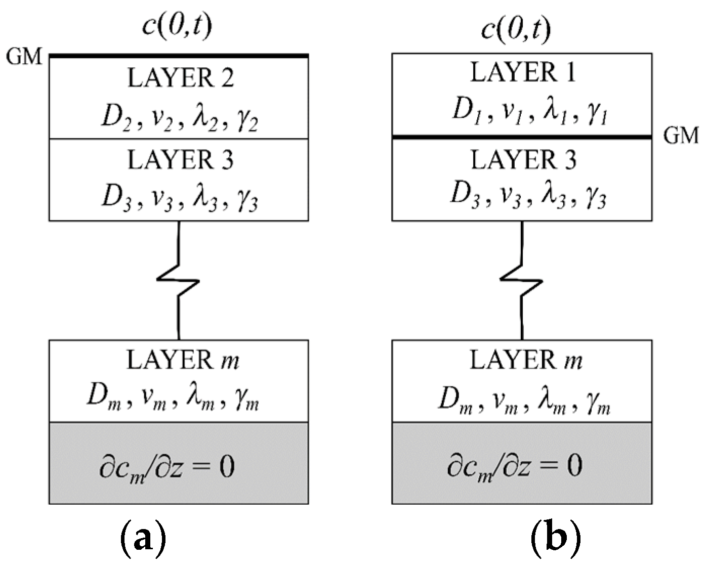
The assumptions of the model proposed are (i) initial concentrations within layers may vary in each material; (ii) the top surface concentration is constant or an arbitrary function of time; (iii) interface concentrations and mass fluxes are continuous between layers; and (iv) the bottom boundary condition implies that the concentration derivative is zero (Neumann boundary condition).
The parameters considered in the model are as follows: the hydrodynamic dispersion coefficient Di of each layer from i = 1, 2, …, m; the molecular diffusion of geomembrane (DGM); the seepage velocity v; the first-order decay constant λ; the zero-order constant γ; and the partition coefficients of the geomembrane SL,GM and S0,GM (Figure 1).

Figure 1.
Schematic diagram of the transport of contaminant through multiple layers: (a) GM as first layer and (b) GM as intermediate layer.
The governing equations and boundary conditions used in this paper are as follows. The transport of contaminants in layer can be expressed using the advection–dispersion–reaction equation [22]:
where t is time (T); z is the direction of the transport of the contaminant (L); Dh,i is the hydrodynamic dispersion coefficient of layer i (L2 T−1); vi is the seepage velocity (LT−1); λi is the first-order decay constant (T−1); γi is the zero-order production/consumption constant (M L−3T−1); and Ri is the retardation factor for linear sorption determined using Equation (2):
where ρdi is the dry density of layer I (ML−3); Kdi is the sorption distribution coefficient of layer i (L3M−1); and θi is the volumetric water content of layer i (L3L−3). In geotechnical engineering, absorption and adsorption (referred to as sorption) can affect the concentration and mobility of solutes [38].
The contaminant biodegradation may be expressed by the first-order decay constant [7]. The decay constant λi is described as a function of the half-life (t1/2,i) of the contaminant [36]:
where t1/2 is the half-life of a contaminant of layer i (T), defined as the time required for the quantity of the contaminant to decay to half of its initial value.
Seepage velocity in a multi-layer system considering the thickness of the contaminant above the m layers is represented by the following Equation (3) [23]:
where hw is the contaminant head (L); li is the thickness of each layer in the system (L); and ke is the effective hydraulic conductivity of the system (LT−1), which is equivalent to the harmonic mean of the hydraulic conductivities of the layers [18]:
where ki is the saturated hydraulic conductivity of layer i (LT−1).
The hydrodynamic dispersion coefficient can be expressed as the sum of the effective coefficient of molecular diffusion Dm,I (L2 T−1) and the dispersion coefficient DD,I (L2 T−1):
The solution to the multi-layer contaminant transport equation depends on the initial and boundary conditions. The initial condition can be expressed as follows [18,23]:
where ci is the initial concentration of the contaminant in layer i (M L−3).
The top boundary condition of the imposed concentration can be approximated by a first-order rate equation [3,36,37]:
where c0 is the peak concentration of the contaminant (M L−3) and λ is the decay constant (T−1) described in Equation (3). When the concentration of the contaminant in the overlying medium is not available, a constant concentration c0 is often applied. Thus, Equation (8) becomes [18,23,24]
In the transport of contaminants in multi-layers (Figure 1), we need to account for the continuity between layers. Hence, the contaminant concentration and dispersive flux are considered continuous at the interfaces between adjacent layers [22]:
When considering the seepage velocity, we obtain [23]
If the first layer is composed of the GM (Figure 1a), then the general transport equation, Equation (1), becomes [18,23,24]
where DGM is the molecular diffusion coefficient of GM (L2 T−1).
At the interface between the GM and contaminant, the inlet boundary condition is [23]
where S0,GM is the partition coefficient that indicates the ratio of the concentration of the contaminant to the concentration in GM.
The interface boundary condition between the GM and underlying SL is defined by the following equation [21]:
where SL,GM is the partition coefficient indicating the ratio of the concentration of the GM contaminant to that in the soil’s pore water at the interface of the two layers.
We now assume that the interface boundary conditions can be described as [23]
The top boundary condition at the inlet (z = 0) becomes
Equation (17) into Equations (15) and (16), we obtain
The GM is not at the top of the system but between two layers (Figure 1b), then Equations (17), (19), and (20) are still valid.
The bottom boundary condition at the last layer is of the following type [18,23,24]:
Based on the initial and boundary conditions and the continuity of the interfaces, the solution of the equation for a multi-layer system can be proposed. In Appendix A, the solution is presented.
Based on the advection and dispersion mass balance, the mass flux J of an arbitrary layer i is [37,39] as follows:
3. Results
3.1. Model Validation
The model was validated using the simulation made by Chen et al. [36]. The authors analyzed data from existing numerical solutions [21,37] to compare with their analytical solutions. The parameters of the CCL were taken from Foose et al. [21], and the parameters of the SL were obtained from Rowe and Booker [37]. All parameters are listed in Table 1 and are related to the toluene contaminant.

Table 1.
Parameters used in the validation of the semi-analytical solution [21,37].
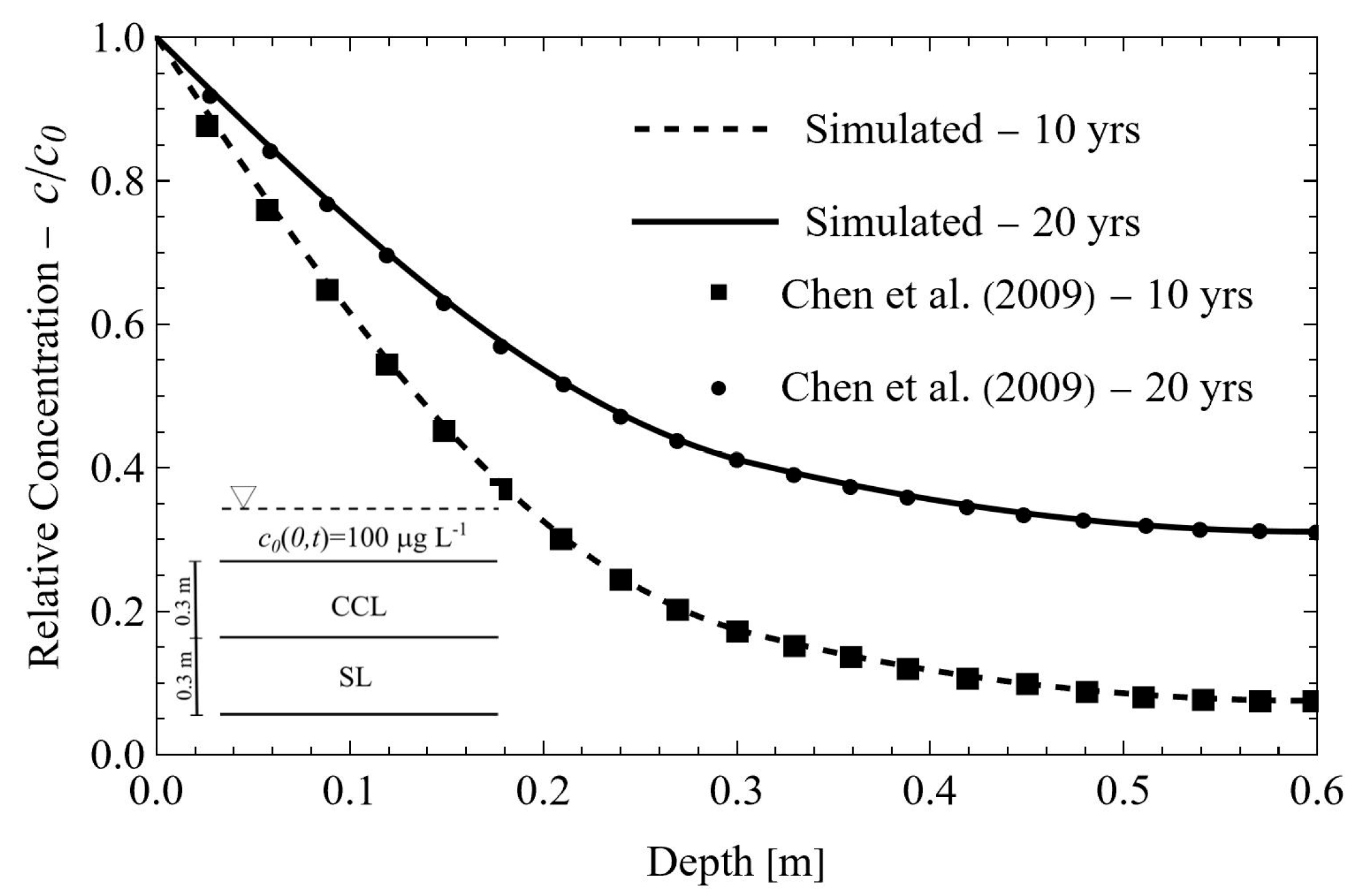
The contaminant concentration profiles of the two-layered soil were compared to the semi-analytical solution (Figure 2) and the solution presented by Chen et al. [36]. The boundary conditions included a zero initial concentration (ci = 0), constant top-surface concentration (cu[0,t] = 100 μg L−1), and a Neumann bottom boundary (Equation (21)). The times (10 and 20 years) are simulation periods often used to design liner systems. The triangle in the lower left corner represents the contaminant head (e.g., leachate).
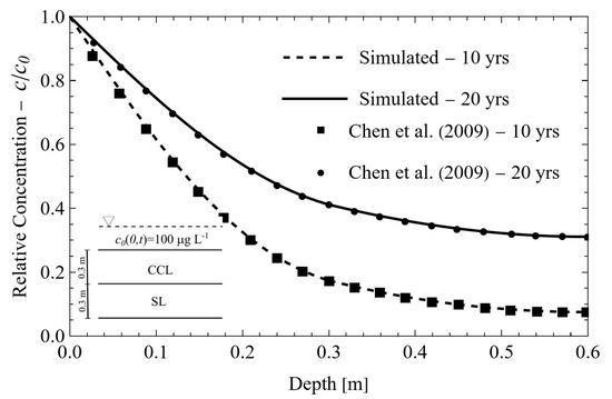
Figure 2.
Comparison of the semi-analytical model and the numerical model of Chen et al. [36].
As shown in Figure 2, the semi-analytical solution used in this research agrees well with other models in the literature, which includes those by Chen et al. [36] and Rowe and Booker [37] (the latter of which was validated by the authors of the former). Benzene and acetone were selected to represent hydrophobic and hydrophilic organic compounds, respectively, as these contaminants are usually found in leachate compounds [36]. Differently from Chen et al. [36], the model in the present study also accounts for the presence of a GM. Figure 3 shows the validation with a GM (1.5 mm) and a CCL (0.6 m). Table 2 presents the simulation parameters along with the values for the high-density polyethylene (HDPE) geomembrane [36]. The results confirm the applicability of the model.
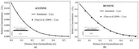
Figure 3.
Validation of the proposed model with the contaminants (a) acetone and (b) benzene [36].
Table 2.
Parameters of materials for the simulation [36].
3.2. Parametric Evaluation
Parametric studies were conducted to validate the versatility of the model under varying conditions, encompassing combinations of compacted clay liners (CCLs), SLs, geomembranes (GMs), and GCLs. Table 3 lists the material parameters for toluene, as documented by Xie et al. [40].
Table 3.
Toluene parameters in GCL, SL, and CCL [40].
Table 4 shows scenarios altering the diffusion coefficient and GM thickness in the presence of a CCL (parameters in Table 3). In the simulation, the values of DGM were 10−11 m2 s−1 for a 0.75 mm HDPE GM [41], 10−13 m2 s−1 for a 1.5 mm HDPE GM [40], and 10−14 m2 s−1 for a 2.5 mm HDPE GM [41]. The values of S0,GM and SL,GM were set to 100. In addition, the dispersion was ignored, as in the studies from where the parameters were obtained.
Table 4.
Scenarios proposed in the parametric analyses [40,41].
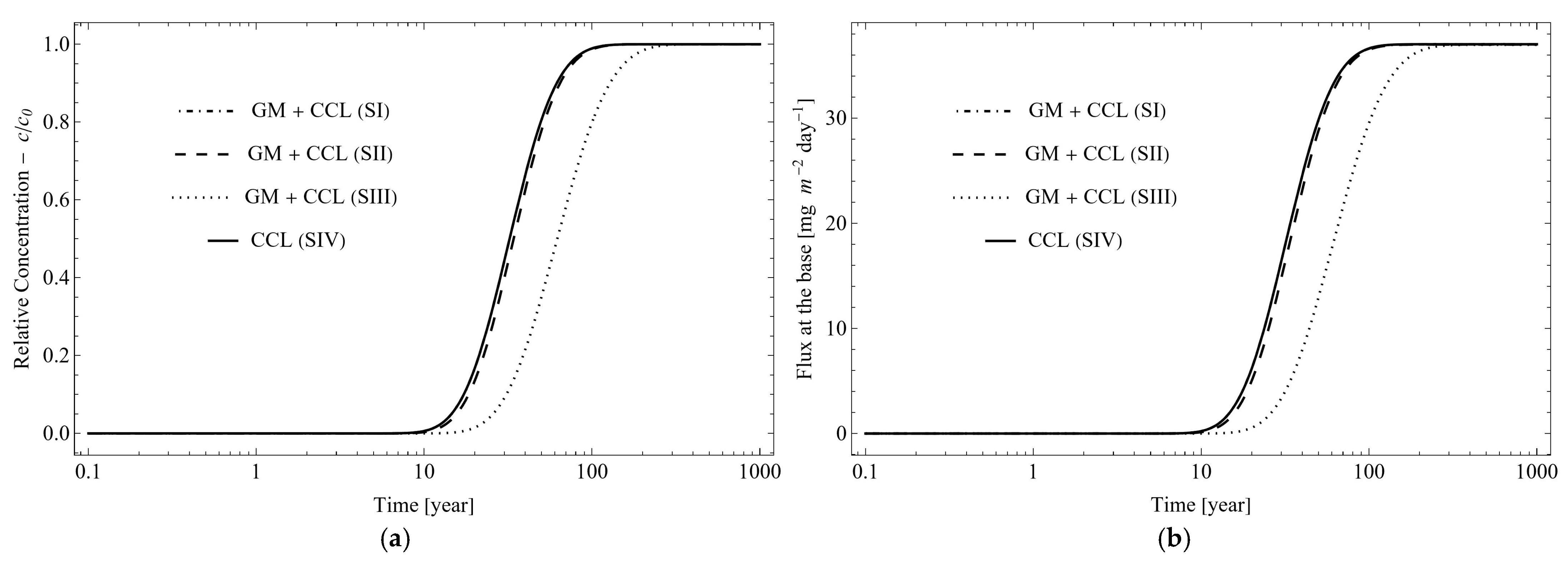
Figure 4 shows values for the relative concentration (Figure 4a) and the flow at the base (Figure 4b) in the four scenarios. The first three scenarios (SI, SII, and SIII) involved constant heads of toluene (0.3 m) and CCL (0.6 m) but used different diffusion coefficients for GM (DGM). For a comparative analysis, scenario SIV, having only a CCL (0.6 m), was considered. The results show that DGM values greater than 10−13 m2 s−1 (SI and SII) exhibited similar efficacies when compared with the presence of CCL alone (SIV). However, DGM = 10−14 m2 s−1 (SIII) proved more efficient than SIV. These analyses show the importance of choosing the most appropriate construction system based on the location and availability of materials. Furthermore, they show the need to obtain DGM with adequate precision to achieve the non-pollution of groundwater. Figure 4b shows the flow at the base of the system.

Figure 4.
Parametric analysis of a two-layer system: (a) relative concentration and (b) flux at the base.
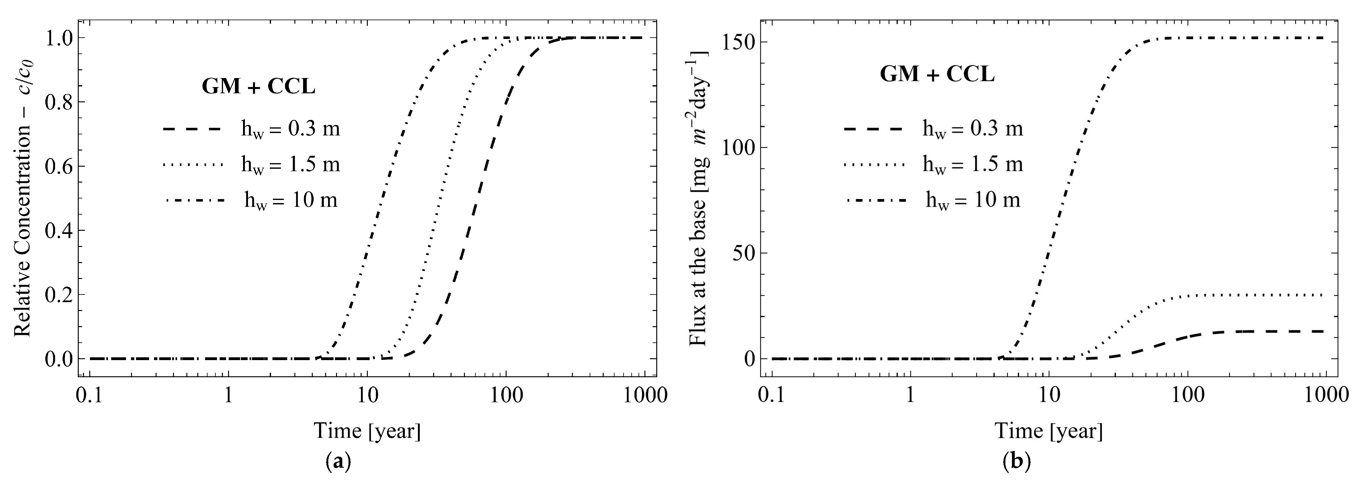
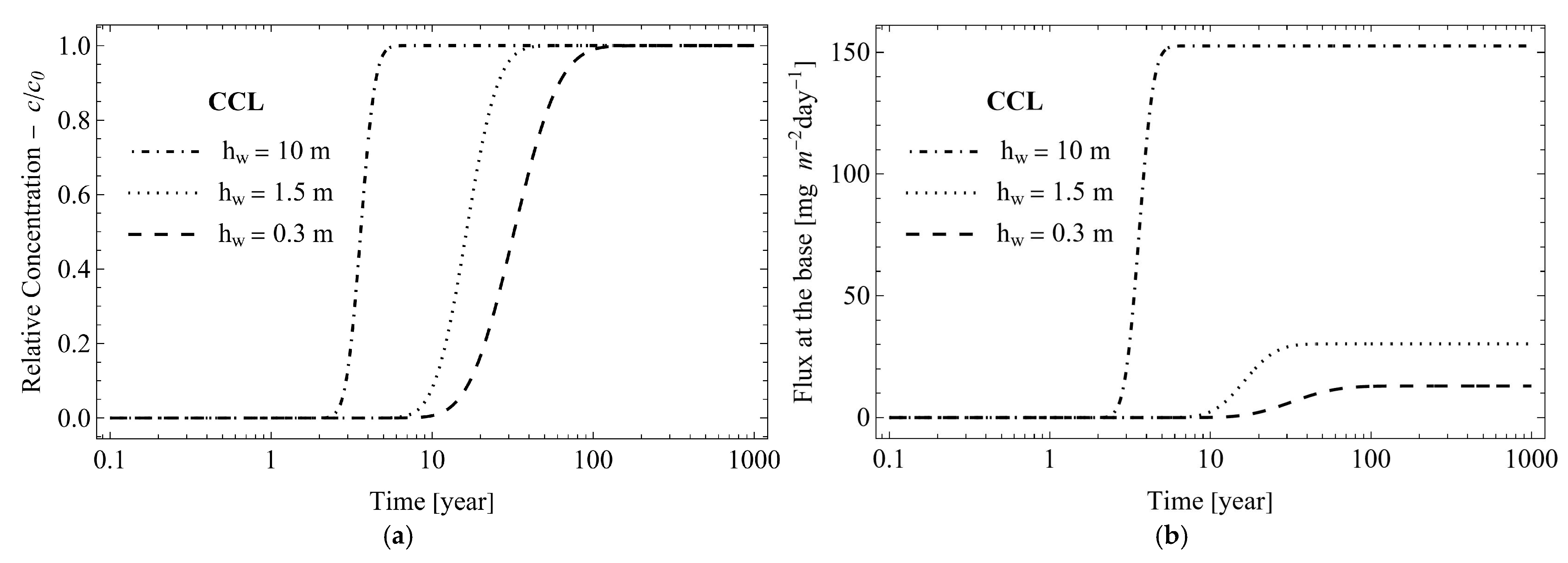
Figure 5 shows a two-layer system composed of a GM and CCL, simulating scenario SIII in Table 4 but with varying toluene head values (hw = 0.3, 1.5, and 10 m). The initial concentration was considered null, and the top boundary condition equaled 100 mg L−1. Figure 5a,b illustrate how the toluene breakthrough curve and the flow were affected, respectively, depending on the head of the contaminant (Equation (4)). Similarly, Figure 6 shows results for only a 0.6 m thick CCL. A comparison of Figure 5 and Figure 6 explains that the GM causes the greater mitigation of contaminant transport. However, depending on the maximum value allowed for the contaminant (e.g., groundwater, soil) and the landfill’s lifespan, sometimes, only CCL may be used.
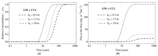
Figure 5.
Toluene transport for different heads: (a) relative concentration and (b) flux at the base.
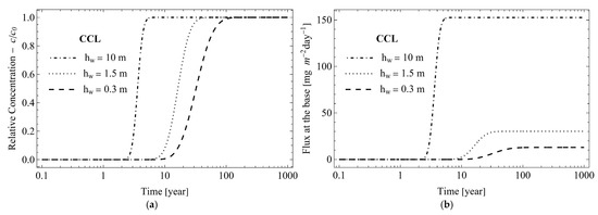
Figure 6.
Toluene transport for different heads: (a) relative concentration and (b) flux at the base.
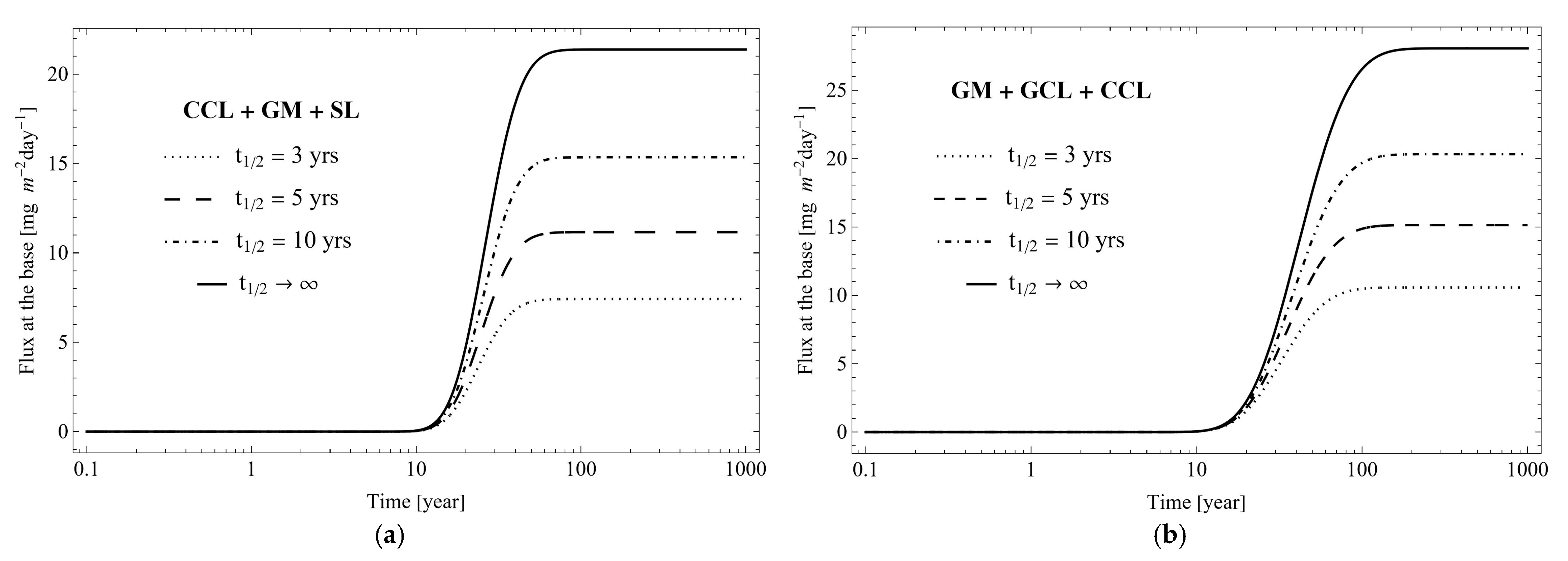
Figure 7 shows the results for a three-layer system using the parameters for CCL and SL presented in Table 3. The GM parameters matched those in scenario SII in Table 4 (DGM = 10−13 m2 s−1 and a thickness of 1.5 mm). In addition, the initial concentration was null, and the upper boundary condition was considered constant at 100 mg L−1 with a toluene head of 0.3 m. Figure 7a illustrates a type of material distribution (CCL, GM, and SL) often used in landfills because of the intercalation of the GM with different soils. Figure 7b shows the intercalation of GM with GCL and a layer of CCL at the base. In both analyses of Figure 7, the contaminant first-order term (decay/biodegradation) was considered only in soil layers (CCL and SL) using Equation (3). Thus, the higher the contaminant half-life t1/2, the greater the flow at the system’s base. In addition, the system formed by CCL, GM, and SL provides a lower flow of toluene, mainly because of the thickness and hydraulic conductivity values of the total system (Figure 7a). However, even with the different thicknesses of GCL (0.01 m) and SL (0.6 m), the change in flow is not significant.
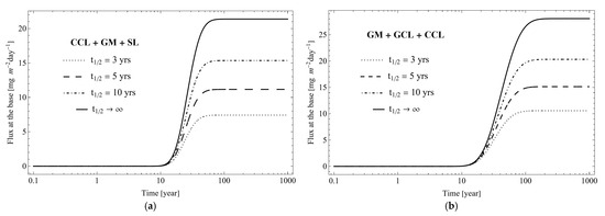
Figure 7.
Toluene flow at the base of three-layer systems: (a) CCL, GM, and SL system; (b) GM, GCL, and CCL system.
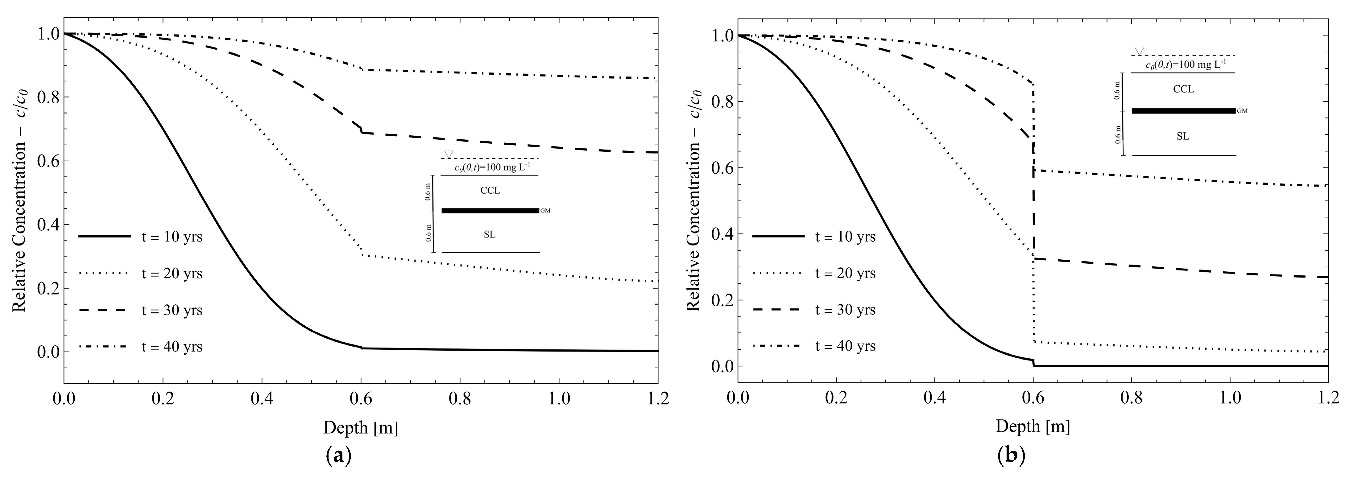
To analyze the difference in GM parameters and their effect on the transport of toluene, relative concentrations were compared, as shown in Figure 8, for a three-layer system (CCL, GM, and SL) with a toluene head of 0.3 m. The parameters used for CCL and SL in Figure 8a,b are found in Table 3. The GM parameters from scenarios SII and SIII (Table 4) are used in Figure 8a,b, respectively. The imposed concentration was 100 mg L−1. Thus, we see that a factor of 10 in DGM causes a significant delay in the contamination front.

Figure 8.
CCL, GM, and SL systems with varying diffusion coefficients of the geomembrane: (a) DGM = 10−13 m2 s−1; (b) DGM = 10−14 m2 s−1.
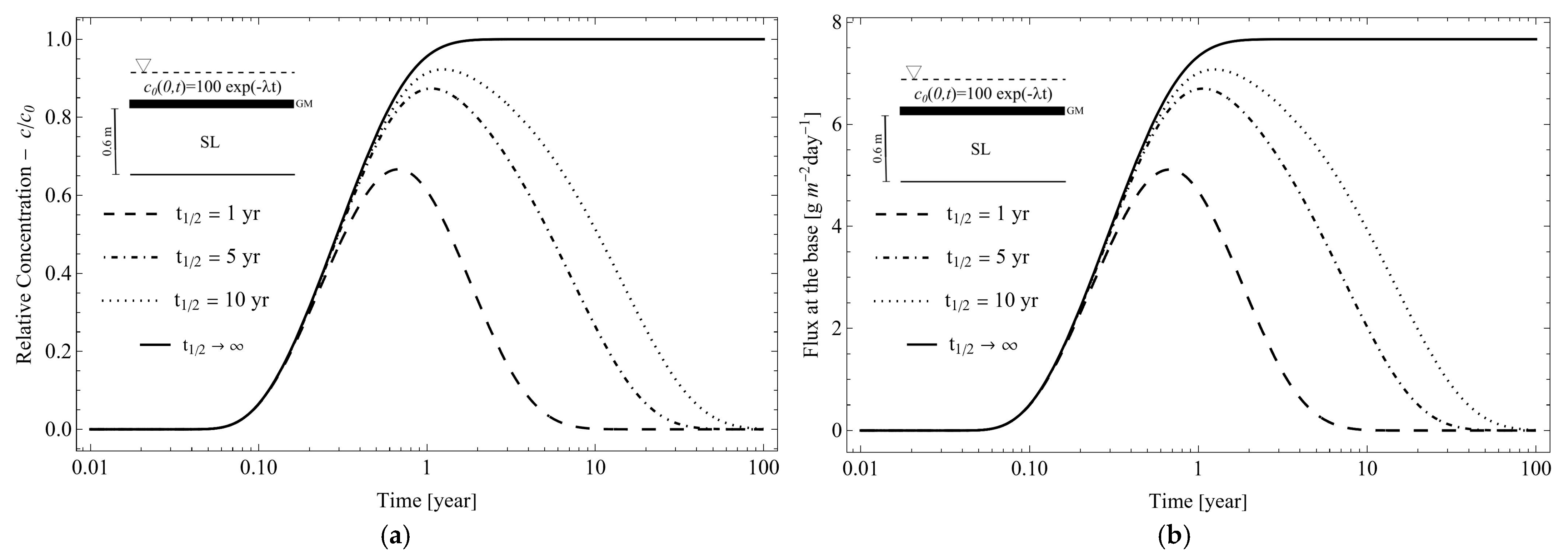
Figure 9 shows a situation in which the upper boundary condition is equal to c0(0, t) = 100 exp (−λt) in a two-layer system (GM + SL) with a different half-life. The first-order term in this analysis was only considered for the boundary condition and not for the SL (Equation (8)). The toluene head was 1 m, the SL parameters are from Table 3, and the GM parameters were from scenario SII (Table 4). For smaller values of t1/2, the decrease was more significant in the toluene breakthrough curve. Therefore, analyses considering this boundary condition must be well evaluated for safety reasons. If t1/2 tends to infinity (solid line in Figure 9), the situation becomes similar to the analyses in Figure 5.
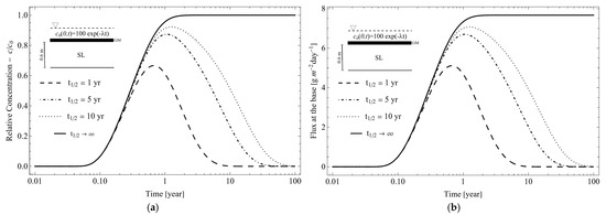
Figure 9.
Imposed concentration with first-order rate equation for different half-lives: (a) relative concentration; (b) flux at the base of the liner system.
The parameters in Table 5 were used to simulate a four-layer system considering the generation of a contaminant (zero-order term). Figure 10 shows the results of an analysis incorporating a protective layer (PL), drainage layer (DL), geomembrane (GM), and a compacted clay liner (CCL). A contaminant was present at the top of the PL (c0 = 100 μL−1), and a zero initial condition was used for all layers. The seepage velocity and the dispersive terms were ignored in all layers. However, a contaminant (γDL > 0) was generated at the DL, indicating problems with this layer. As shown in Figure 10, the flux changed by a factor of ten, comparing the non-generation (γDL = 0) with the highest generation considered (γ = 10−2). This result shows the value of knowing the presence of a contaminant that can alter the flux in the system significantly.
Table 5.
Material parameters according to Xie et al. [40].
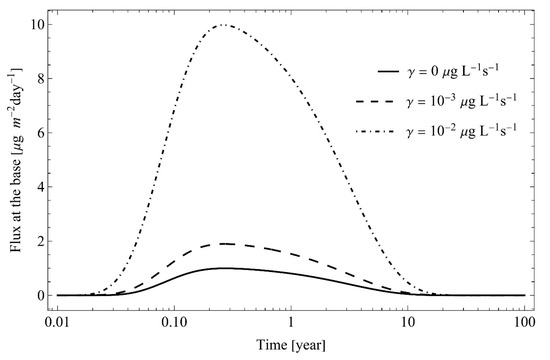
Figure 10.
Flux of contaminant considering generation (zero-order term).
3.3. Application to Real Sanitary Landfill
The model developed was applied in a real sanitary landfill to verify its performance. The case study was the Brasília Sanitary Landfill (BSL), located in the capital of Brazil. The BSL was opened on 17 January 2017. As of June 2023, the BSL has already received 4,212,142 tons of waste [42]. The BSL’s liner system comprises a triple layer of 0.5 m topsoil CCL (CCL1) above an HDPE geomembrane that overlays a 1.5 m thick CCL (CCL2) layer. The current total clay thickness is 2 m and the life span of the BSL is 13 years.
All parameters of the landfill materials for the benzene contaminant are shown in Table 6, as mentioned in Baran [43]. To assess the performance of the geomembrane with an extra layer of clay, the parameters shown for CCL3 were defined.
Table 6.
Material parameters for the benzene contaminant [43].
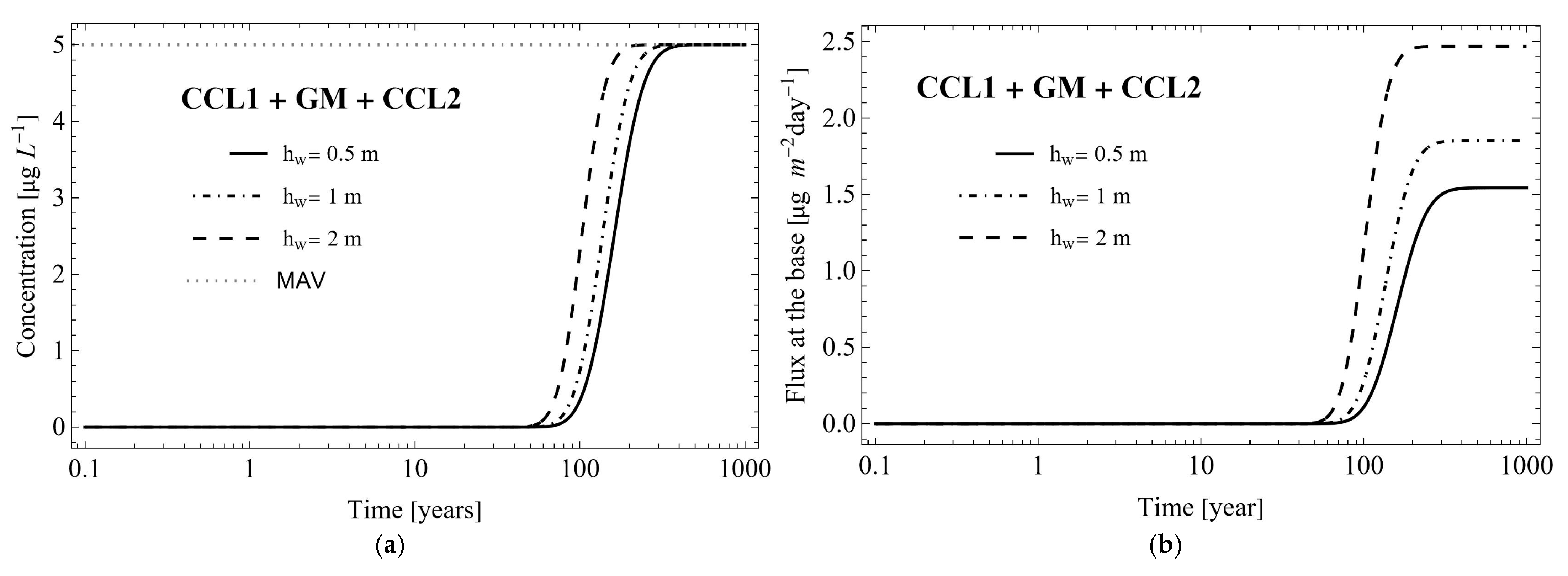
Breakthrough and flow curves for different benzene heads (0.5, 1, and 2 m) were evaluated in a three-layer system, as shown in Figure 11. The initial concentration of the contaminant was considered null. The upper boundary condition was considered constant at 5 μg L−1, the maximum allowed value (MAV) for water potability according to Brazilian standards [44].
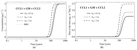
Figure 11.
Contaminant transport in possible multi-liner system for the BSL: (a) concentration profile; (b) flux in a three-layer system.
The benzene concentration reached the MAV after 100 years of simulation for all benzene heads. The landfill was designed for a lifespan of approximately 13 years. Therefore, the designed liner is effective against benzene transport, exhibiting good performance. The model can be applied for the most critical contaminants in the leachate of the site to assess safety against groundwater contamination.
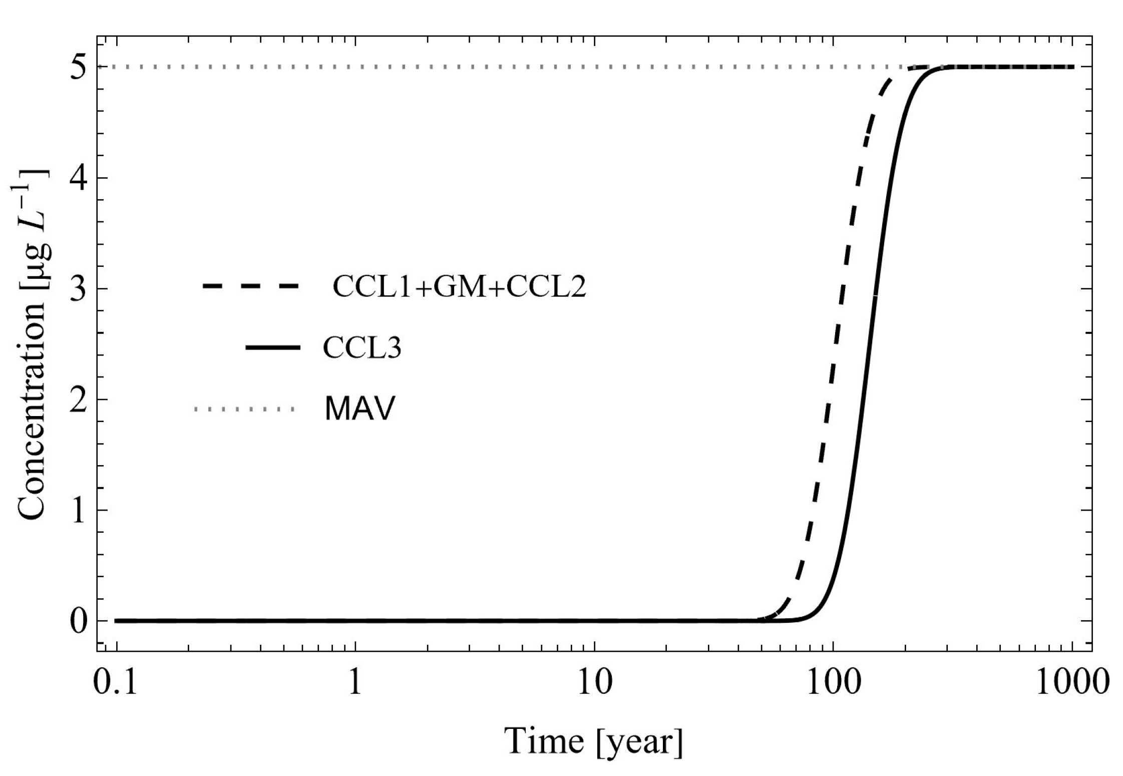
Using the values in Table 6, we compared the current construction system of BSL (CCL1, GM, and CCL2) with a system including only one CCL layer of 2.5 m (CCL3) and a benzene head of 2 m. The comparative layer did not contain GM. Figure 12 shows the breakthrough curve of the current landfill system (dashed line) and the modified system (continuous line). The result shows that adding 0.5 m of soil thickness results in a more effective system—without GM—for a period longer than 50 years, which is significantly greater than the expected lifespan of the landfill. However, a cost–benefit analysis must be carried out before the optimal construction system can be defined.

Figure 12.
Comparison of constructive models of landfill liners.
4. Conclusions
Analytical models of contaminant transport are robust tools for parametric and numerical validation. Notably, both analytical and semi-analytical approaches maintain continuity across spatial and temporal domains. This research extends a semi-analytical model of the advection–dispersion–reaction equation to encapsulate these benefits.
Model validation, employing materials such as compacted clay liners (CCLs), SLs, GCLs, and geomembranes (GMs), effectively demonstrated the model’s capability to simulate multi-layer systems. The inherent heterogeneity of these materials indicates their critical importance when designing geostructures, especially landfill liners. The accurate comprehension of the transport of contaminants (like leachate) is pivotal for refining these geostructural designs.
The use of analytical and semi-analytical models eases parametric analysis greatly. Our research indicates the value of determining the geomembrane’s diffusion coefficient through lab analyses, facilitating an accurate prediction of contaminant transport and highlighting the trade-offs between opting for a geomembrane (GM) or augmenting the thickness of traditional soil liners (e.g., CCLs and SLs). Regardless, the geomembrane’s essential role as an advective flow barrier remains undebatable, necessitating rigorous checks to ensure its integrity. Moreover, incorporating first-order (decay/biodegradation) and zero-order (species source) terms is critical for a holistic prediction of contaminant transport dynamics.
The open-source model introduced here may be regarded as a versatile tool for simulating multi-layer systems to aid in optimizing landfill liner designs and thus contributing directly to minimizing soil contamination and mitigating groundwater pollution. Aiming for more comprehensive application, future research should investigate the applicability of the solution comparing with laboratory results analyzing multilayers of materials. Furthermore, for a holistic consideration of the contaminant transport phenomenon, the implementation of the material saturation (CCL and SL) and temperature in the model is recommended.
Author Contributions
Conceptualization, M.A.C.L.; methodology, M.A.C.L. and A.L.B.C.; validation, M.A.C.L. and C.T.B.; formal analysis, M.A.C.L.; investigation, M.A.C.L., C.T.B. and E.M.P.; resources, M.A.C.L.; data curation, M.A.C.L. and A.L.B.C.; writing—original draft preparation, M.A.C.L.; writing—review and editing, M.A.C.L., C.T.B., A.L.B.C. and E.M.P.; visualization, M.A.C.L., C.T.B. and E.M.P.; supervision, A.L.B.C. and E.M.P.; project administration, A.L.B.C. and E.M.P.; funding acquisition, M.A.C.L. and A.L.B.C. All authors have read and agreed to the published version of the manuscript.
Funding
This study was partially funded by the Coordination for the Improvement of Higher Education Personnel—Brazil (CAPES)—Finance Code 001, the National Council for Scientific and Technological Development (CNPq Grant 435962/2018-3, 140923/2020-9, 305484/2020-6) and the Foundation for Research Support of the Federal District (FAPDF) (Project 00193-00001609/2023-44).
Data Availability Statement
All data, models, and code that support this study’s findings are available from the corresponding author upon reasonable request.
Conflicts of Interest
The authors declare no conflict of interest.
Appendix A
Appendix A.1. General Solution for m Layers in Laplace Space
Considering the extension of the solution for a system with m layers and the solution for each layer i in the Laplace space as follows:
Both G0(s) = {g0(t)} and GL(s) = {gL(t)} are assumed to be found analytically. The auxiliary functions Ai, Bi, and Pi (i = 1, …, m) are presented below.
The advection–dispersion–reaction equation (Equation (1)) is vital for studying contaminant transport in multi-layered systems. The solution adopted in the present study considered general boundary conditions at the inlet (z = 0) and outlet (z = L) [22]:
Boundary conditions of Equations (A4) and (A5) (i.e., a0, b0, aL, and bL) are constants; g0(t) and gL(t) are auxiliary functions with the subscripts 0 and L denoting the top and bottom, respectively, of the landfill liner. Using Equation (8), we obtain a0 = 1, b0 = 0, and g0(t) = c0 exp (−λt). However, Equation (9) yields a0 = 1, b0 = 0, and g0(t) = c0. Finally, Equation (21) gives aL = 0, bL = 1, and gL(t) = 0.
First layer (i = 1):
In cases involving the presence of a geomembrane, the term θ1 × D1 must be changed to SL,GM × DGM.
Middle layer (i = 2, …, m − 1):
In cases involving the presence of a geomembrane, the term θi × Di must be changed to SL,GM × DGM.
Last layer (i = m):
In cases involving the presence of a geomembrane, the term θm × Dm must be changed to SL,GM × DGM.
For all layers (i = 1, …., m):
The determination of G1(s),…, Gm−1(s) is obtained based on the continuity of concentration at each interface in the Laplace domain [22,45,46,47]:
Incorporating Equations (A1)–(A3) into the system of equations (Equation (A23)) yields a linear system for x = [G1(s),…, Gm−1(s)]T:
where A = (ai,j) ℂ(m−1)x(m−1) is a tridiagonal matrix and b = (bi) ℂ(m−1) is a vector with the entries described in Equation (A23).
Simplification of two layers
The model presented in the previous section differs in the case of a two-layer system because of the assumption of middle layers. The concentrations of the two layers in the Laplace domain become [22]
Defined entries of the linear system Equation (A23) are no longer valid for m = 2. In this case, the linear system reduces to the following:
Because of the complexity involved in converting the solution from Laplace space to z and t space, a numerical solution is proposed based on the assumption of Trefethen et al. [47] to compute the inverse Laplace transform [22]:
where N is even; ON is the set of positive odd integers less than N; sk = zk/t and wk, sk ∈ ℂ are the residues and poles, respectively, of the best (N, N) rational approximation to ez on the negative real line [22]. Both wk and zk are constants that can be computed using a supplied function [47].
Appendix A.2. Flux of Contaminant of an Arbitrary Layer
Applying the mass flux described in Equation (22) and incorporating Equation (A29), we obtain the following:
References
- Wijekoon, P.; Koliyabandara, P.A.; Cooray, A.T.; Lam, S.S.; Athapattu, B.C.L.; Vithanage, M. Progress and prospects in mitigation of landfill leachate pollution: Risk, pollution potential, treatment and challenges. J. Hazard. Mater. 2022, 421, 126627. [Google Scholar] [CrossRef]
- Lu, S.-F.; Xiong, J.-H.; Feng, S.-J.; Chen, H.-X.; Bai, Z.-B.; Fu, W.-D.; Lü, F. A finite-volume numerical model for bio-hydro-mechanical behaviors of municipal solid waste in landfills. Comput. Geotech. 2019, 109, 204–219. [Google Scholar] [CrossRef]
- Rowe, R.K.; Quigley, R.M.; Brachman, R.W.I.; Booker, J.R. Barrier Systems for Waste Disposal Facilities; Taylor & Francis: London, UK, 2004. [Google Scholar]
- Bernardo, B.; Candeias, C.; Rocha, F. Characterization of the Dynamics of Leachate Contamination Plumes in the Surroundings of the Hulene-BWaste Dump in Maputo, Mozambique. Environments 2022, 9, 19. [Google Scholar] [CrossRef]
- Christensen, T.H.; Kjeldsen, P.; Bjerg, P.L.; Jensen, D.L.; Christensen, J.B.; Baun, A.; Albrechtsen, H.J.; Heron, C. Biogeochemistry of landfill leachate plumes. Appl. Geochem. 2001, 16, 659–718. [Google Scholar] [CrossRef]
- Jiang, Y.; Li, R.; Yang, Y.; Yu, M.; Xi, B.; Li, M.; Xu, Z.; Gao, S.; Yang, C. Migration and evolution of dissolved organic matter in landfill leachate-contaminated groundwater plume. Resour. Conserv. Recycl. 2019, 151, 104463. [Google Scholar] [CrossRef]
- Guan, C.; Xie, H.J.; Wang, Y.Z.; Chen, Y.M.; Jiang, Y.S.; Tang, X.W. An analytical model for solute transport through a GCL-based two-layered liner considering biodegradation. Sci. Total Environ. 2014, 466–467, 221–231. [Google Scholar] [CrossRef]
- Southen, J.M.; Rowe, R.K. Evaluation of the water retention curve for geosynthetic clay liners. Geotext. Geomembr. 2007, 25, 2–9. [Google Scholar] [CrossRef]
- Özçoban, M.S.; Acarer, S.; Tüfekci, N. Effect of solid waste landfill leachate contaminants on hydraulic conductivity of landfill liners. Water Sci. Technol. 2022, 85, 1581–1599. [Google Scholar] [CrossRef]
- McWatters, R.S.; Rutter, A.; Rowe, R.K. Geomembrane applications for controlling diffusive migration of petroleum hydrocarbons in cold region environments. J. Environ. Manag. 2016, 181, 80–94. [Google Scholar] [CrossRef]
- Rowe, R.K. Long-term performance of contaminant barrier systems. Géotechnique 2005, 55, 631–678. [Google Scholar] [CrossRef]
- Shackelford, C.D. The ISSMGE Kerry Rowe Lecture: The role of diffusion in environmental geotechnics. Can. Geotech. J. 2014, 51, 1219–1242. [Google Scholar] [CrossRef]
- EPA625-4-89-022; Requirements for Hazardous Waste Landfill Design, Construction, and Closure. U.S. EPA: Washington, DC, USA, 1989.
- Bouazza, A.; Bowders, J.J. Geosynthetic Clay Liners for Waste Containment Facilities; Taylor & Francis Group: London, UK, 2010. [Google Scholar]
- Shan, H.-Y.; Lai, Y.-J. Effect of hydrating liquid on the hydraulic properties of geosynthetic clay liner. Geotext. Geomembr. 2002, 20, 19–38. [Google Scholar] [CrossRef]
- Uma Shankar, M.; Muthukumar, M. Comprehensive review of geosynthetic clay liner and compacted clay liner. IOP Conf. Ser. Mater. Sci. Eng. 2017, 263, 032026. [Google Scholar] [CrossRef]
- Visentin, C.; Zanella, P.; Kronhardt, B.K.; Da Silva Trentin, A.W.; Braun, A.B.; Thomé, A. Use of geosynthetic clay liner as a waterproofing barrier in sanitary landfills. J. Urban Environ. Eng. 2019, 13, 115–124. [Google Scholar] [CrossRef]
- Giroud, J.; Badu-Tweneboah, K.; Soderman, K.L. Comparison of leachate flow through compacted clay liners and geosynthetic clay liners in landfill liner systems. Geosynth. Int. 1997, 4, 391–431. [Google Scholar] [CrossRef]
- EPA530-F-97-002; Geosynthetic Clay Liners Used in Municipal Solid Waste Landfills. U.S. EPA: Washington, DC, USA, 2001.
- Cleall, P.J.; Li, Y.C. Analytical solution for diffusion of VOCs through composite landfill liners. J. Geotech. Geoenviron. Eng. 2011, 137, 850–854. [Google Scholar] [CrossRef]
- Foose, G.J. Transit-time design for diffusion through composite liners. J. Geotech. Geoenviron. Eng. 2002, 128, 590–601. [Google Scholar] [CrossRef]
- Carr, E.J. New Semi-Analytical Solutions for Advection–Dispersion Equations in Multilayer Porous Media. Transp. Porous Medium 2020, 135, 39–58. [Google Scholar] [CrossRef]
- Xie, H.; Zhang, C.; Sedighi, M.; Thomas, H.R.; Chen, Y. An analytical model for diffusion of chemicals under thermal effects in semi-infinite porous media. Comput. Geotech. 2015, 69, 329–337. [Google Scholar] [CrossRef]
- Xie, H.; Chen, Y.; Lou, Z. An analytical solution to contaminant transport through composite liners with geomembrane defects. Sci. China Technol. Sci. 2010, 53, 1424–1433. [Google Scholar] [CrossRef]
- Ozelim, L.C.S.M.; Paz, Y.P.L.; Cunha, L.S.; Cavalcante, A.L.B. Enhanced landfill’s characterization by using an alternative analytical model for diffusion tests. Environ. Monit. Assess. 2021, 193, 739. [Google Scholar] [CrossRef]
- Xie, H.J.; Thomas, H.R.; Chen, Y.M.; Sedighi, M.; Tang, X.W. Diffusion of organic contaminants in triple-layer composite liners—An analytical modelling approach. Acta Geotech. 2015, 10, 255–262. [Google Scholar] [CrossRef]
- Peng, M.-Q.; Feng, S.-J.; Chen, H.-X.; Chen, Z.-L. An analytical solution for organic pollutant diffusion in a triple-layer composite liner considering the coupling influence of thermal diffusion. Comput. Geotech. 2021, 137, 104283. [Google Scholar] [CrossRef]
- Qiu, J.; He, Y.; Song, D.; Tong, J. Analytical solution for solute transport in a triple liner under non-isothermal condition. Geosynth. Int. 2022, 30, 364–381. [Google Scholar] [CrossRef]
- Lin, H.; Huang, W.; Wang, L.; Liu, Z. Transport of Organic Contaminants in Composite Vertical Cut-Off Wall with Defective HDPE Geomembrane. Polymers 2023, 15, 3031. [Google Scholar] [CrossRef] [PubMed]
- Davis, G.B.; Patterson, B.M.; Johnston, C.D. Aerobic bioremediation of 1, 2 dichloromethane and vinyl chloride at field scale. J. Contam. Hydrol. 2009, 107, 91–100. [Google Scholar] [CrossRef] [PubMed]
- Wiedemeier, T.H.; Rifai, H.S.; Newell, C.J.; Wilson, J.T. Natural Attenuation of Fuels and Chlorinated Solvents in the Subsurface; Wiley: New York, NY, USA, 1999. [Google Scholar]
- Ogata, A.; Banks, R.B. A Solution of the Differential Equation of Longitudinal Dispersion in Porous Media; U.S. Government Printing Office: Washington, DC, USA, 1961.
- Van Genuchten, M.T.; Alves, W.J. Analytical Solutions of the One-Dimensional Convective-Dispersive Solute Transport Equation; U.S. Department of Agriculture, Agricultural Research Service: Washington, DC, USA, 1982.
- Leij, F.J.; Van Genuchten, M.T. Approximate analytical solutions for solute transport in two-layer porous media. Transp. Porous Med. 1995, 18, 65–85. [Google Scholar] [CrossRef]
- Liu, C.; Ball, W.P.; Ellis, J.H. An analytical solution to the one-dimensional solute advection-dispersion equation in multi-layer porous media. Transp. Porous Med. 1998, 30, 25–43. [Google Scholar] [CrossRef]
- Chen, Y.; Xie, H.; Ke, H.; Chen, R. An analytical solution for one-dimensional contaminant diffusion through multi-layered system and its applications. Environ. Geol. 2009, 58, 1083–1094. [Google Scholar] [CrossRef]
- Rowe, R.K.; Booker, J.R. The analysis of pollutant migration in a non-homogeneous soil. Geotechnique 1984, 34, 601–612. [Google Scholar] [CrossRef]
- Vieira, G.M.D.; Lemos, M.A.C.; Cavalcante, A.L.B.; Casagrande, M.D.T. Effectiveness of Polyvinylidene Fluoride Fibers (PVDF) in the Diffusion and Adsorption Processes of Atrazine in a Sandy Soil. Sustainability 2023, 15, 11729. [Google Scholar] [CrossRef]
- Lu, C.S.J.; Morrison, R.D.; Stearns, R.J. Leachate production and management from municipal landfills: Summary and assessment. Land disposal: Municipal solid waste. In Proceedings of the 7th Annual Research Symposium, Philadelphia, PA, USA, 16–18 March 1981. [Google Scholar]
- Xie, H.; Jiang, Y.; Zhang, C.; Feng, S. An analytical model for volatile organic compound transport through a composite liner consisting of a geomembrane, a GCL, and a soil liner. Environ. Sci. Pollut. Res. 2015, 22, 2824–2836. [Google Scholar] [CrossRef] [PubMed]
- Rowe, R.; Hrapovic, L.; Kosaric, N. Diffusion of Chloride and Dichloromethane through an HDPE Geomembrane. Geosynth. Int. 1995, 2, 507–536. [Google Scholar] [CrossRef]
- SLU—Municipal Cleaning Service of the Federal District. January–June 2023, Activity Report of the DF Municipal Cleaning Service; The DF Urban Cleaning Services (SLU): Brasília, Brazil, 2023; 139p. [Google Scholar]
- Baran, C.T. Modeling Contaminant Transport in Multi-Layer Compacted Clay Liners and Geomembrane Liners. Master’s Dissertation, University of Brasília, Brasília, Brazil, 2021. [Google Scholar]
- Brazil—National Environmental Council. Resolution No 396, April 3rd. Published in DOU no. 66, of 7 April 2008, Section 1, pages 64–68. Available online: https://www.mpf.mp.br/atuacao-tematica/ccr4/dados-da-atuacao/projetos/qualidade-da-agua/legislacao/resolucoes/resolucao-conama-no-396-de-3-de-abril-de-2008/view (accessed on 9 October 2023).
- Carr, E.J.; March, N.G. Semi-analytical solution of multilayer diffusion problems with time-varying boundary conditions and general interface conditions. Appl. Math. Comput. 2018, 333, 286–303. [Google Scholar] [CrossRef]
- Carr, E.J.; Turner, I.W. A semi-analytical solution for multilayer diffusion in a composite medium consisting of a large number of layers. Appl. Math. Model. 2016, 40, 7034–7050. [Google Scholar] [CrossRef]
- Trefethen, L.N.; Weideman, J.A.C.; Schmelzer, T. Talbot quadratures and rational approximations. BIT Numer. Math. 2006, 46, 653–670. [Google Scholar] [CrossRef]


Disclaimer/Publisher’s Note: The statements, opinions and data contained in all publications are solely those of the individual author(s) and contributor(s) and not of MDPI and/or the editor(s). MDPI and/or the editor(s) disclaim responsibility for any injury to people or property resulting from any ideas, methods, instructions or products referred to in the content. |
© 2023 by the authors. Licensee MDPI, Basel, Switzerland. This article is an open access article distributed under the terms and conditions of the Creative Commons Attribution (CC BY) license (https://creativecommons.org/licenses/by/4.0/).