Truck-Drone Pickup and Delivery Problem with Drone Weight-Related Cost

Abstract

Truck-drone delivery is widely used in logistics distribution for achieving sustainable development, in which drone weight greatly affects transportation cost. Thus, we consider a new combined truck-drone pickup and delivery problem with drone weight-related cost in the context of last-mile logistics. A system of integer programming is formulated with the objective of minimizing the total cost of the drone weight-related cost, fixed vehicle cost and travel distance cost. An improved adaptive large neighborhood search algorithm (IALNS) is designed based on the characteristics of the problem, several effective destroy and repair operators are designed to explore the solution space, and a simulated annealing strategy is introduced to avoid falling into the local optimal solution. To evaluate the performance of the IALNS algorithm, 72 instances are randomly generated and tested. The computational results on small instances show that the proposed IALNS algorithm performs better than CPLEX both in efficiency and effectiveness. When comparing the truck-drone pickup and delivery problem with drone weight-related cost to the problem without drone weight-related cost, it is found that ignoring the drone weight constraints leads to an underestimate of the total travel cost by 12.61% based on the test of large instances.

1. Introduction

Driven by the constantly increasing demand for flexibility and sustainability in the e-commerce industry, green transportation is gradually gaining attention [1] and drone delivery is demonstrating commercial potential due to its benefits in speed, green emissions, and lack of restrictions from traditional road networks. In particular, unlike trucks, drones excel in the abilities to navigate freely, bypass traffic congestion and emit less carbon dioxide, and require fewer human resources, which contributes to the improvement of logistics efficiency and the reduction of pollution, and further promotes the green and sustainable development of the logistics industry. Many major e-commerce players have joined this trend, using drones for last-mile logistics, including companies like Amazon, DHL, and Google, which have already initiated experimental trials and are progressively establishing drone delivery systems [2,3,4].

Any operation involving drones can be seen as a variant of the vehicle routing problem (VRP), where the optimization objective is to find the best set of routes. However, drones are subject to unique factors, such as limited payload and capped battery capacity [5], which can restrict their use. Therefore, drones often rely on supplementary support, such as trucks or transshipment stations, for launch, landing, reloading, and recharging. To successfully implement drones within urban logistics services, effective strategies must be employed to coordinate these resources effectively. The truck-drone joint delivery mode is a commonly discussed solution, gaining significant attention from both professionals and researchers, which was proposed by Murray and Chu in 2015 [6]. Murray and Chu [6] constructed the model of the traveling salesman problem with drones. Bouman et al. [7] also studied the drone routing problem and designed exact solution approaches; experimental comparison of these approaches was also carried out. Wang et al. [8] focused on the truck-drone joint delivery problem and demonstrated that, even in the worst cases, the truck-drone joint delivery time is shorter than that of truck-only delivery. David et al. [9] and El-Adle et al. [10] also studied the truck-drone joint delivery problem, then proposed an adaptive large neighborhood search algorithm (ALNS) and a branch and bound algorithm to solve it, respectively.

The pickup and delivery problem (PDP) is a widely used combinatorial optimization problem applied across multiple industries, including logistics and robotics [11]. It involves two types of nodes, pickup nodes and delivery nodes, where the former supplies a number of goods for the latter to demand. The goal of the PDP is to identify the most efficient routes to meet the demands of all nodes. Alyasiry et al. [12] designed an exact algorithm to solve the PDP with time windows (PDPTW). Wang et al. [13] also studied the PDPTW, and developed a two-stage heuristic solution algorithm. Ropke and Pisinger [14] proposed an ALNS algorithm for solving the PDPTW, the results demonstrating the effectiveness of the ALNS algorithm. Sartori and Buriol [15] introduced an improved hybrid algorithm, along with a new approach that generates instances based on the open data. Naccache et al. [16] presented a variant of the PDPTW, then an ALNS algorithm with improved operations was developed to tackle this problem. Goeke [17] proposed the electric PDPTW and applied an improved tabu search solution algorithm. Liu et al. [18] studied a granularity-based split PDP, and solved it by an improved genetic algorithm. Hornstra et al. [19] introduced a VRP with simultaneous pickup and delivery, and designed an ALNS solution algorithm.

In truck-drone delivery, both the travel distance and cargo weight are important factors in cost. Especially, the drone weight directly affects energy consumption and resource utilization due to the limited flight range and capacity. The traditional vehicle routing problem only aims to minimize the travel distance cost, resulting in a certain deviation between the actual transportation cost and the optimization cost. Therefore, it is vital to take into account the effect of cargo weight on cost. Researchers have conducted several studies on the VRP considering the cargo weight. Lurkin and Schyns [20] studied the airline container loading PDP, and a mixed integer linear program model was formulated. To solve the PDPTW considering the cargo weight, Hochstenbach et al. [21] developed a branch and price algorithm. Luo et al. [22] addressed the VRP with uncertain demands and cargo weight costs, and designed a priori optimization. Kuo [23] introduced the cargo weight, travel speed and travel distance as factors affecting the fuel consumption in the objective function, and solved it by a simulated annealing algorithm. Zhang et al. [24] constructed an optimization model of the VRP with cargo weight and adopted a scatter search algorithm. Luo et al. [25] proposed the split-delivery VRP with linear weight-related cost and designed an exact branch and price and cut algorithm. Mulati et al. [26] studied the cumulative VRP with cargo weight and proposed the arc-item-load and related formulations for the cumulative VRP. Pan et al. [27] studied the VRP considering random demand and changing load, and constructed a formulation based on the relationship between energy consumption and changing load. Jeong et al. [28] constructed a mathematical model for the VRP considering drone weight-related energy consumption and designed a two-stage heuristic algorithm.

Based on the above discussions, it can be found that, in the existing studies on truck-drone pickup and delivery problem, there is almost no research that considers the impact of drone weight on the total cost. To better fit the practical situation and fill this gap, this paper considers a truck-drone pickup and delivery problem with drone weight-related cost (TDPDP-DW). Based on minimizing the sum of the drone weight-related cost, the fixed vehicle cost, and the travel distance cost, we propose a mixed-integer programming model. On the one hand, we introduce drone delivery into the traditional distribution network. On the other hand, the most economical truck-drone distribution routes are found by optimizing the objective function. All of these help to save energy, promote the effective allocation of resources, reduce the total amount of carbon emissions, and promote the sustainable development of the logistics economy. An improved adaptive large neighborhood search algorithm is designed to solve the problem. Numerical experiments are carried out, verifying the performance of our proposed approach.

The contributions of this paper are summarized as follows:

(i)

To the best of our knowledge, it is the first study to introduce drone weight-related cost into the truck-drone pickup and delivery problem, and the corresponding problem is called the truck-drone pickup and delivery problem with drone weight-related cost. Based on minimizing the sum of the drone weight-related cost, the fixed vehicle cost, and the travel distance cost, a mixed-integer programming model is proposed.

(ii)

To tackle the problem, an improved ALNS algorithm is designed. In this algorithm, several effective destroy operators and repair operators are designed, based on the characteristics of the problem, to explore the solution space, and the simulated annealing acceptance criterion is introduced to improve the algorithm performance by preventing the solution falling into local optima.

(iii)

Extensive computational experiments demonstrate the effectiveness of the model and algorithm and the necessity to consider the drone weight-related cost constraints.

2. Problem Definition and Mathematical Model

The research problem can be described as follows:

(i)

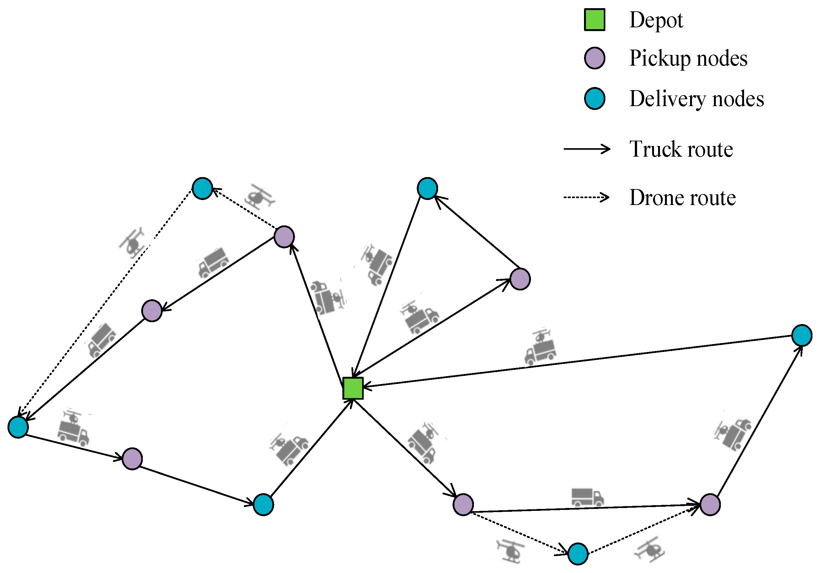
A fleet of identical truck-drone pairs K will begin at 0 and return to 2n + 1 while fulfilling demands for pickup or delivery goods at different locations within specified time windows. The truck’s cargo load must not exceed Q and the drone’s cargo load must not exceed Q’.

(ii)

Customers should be serviced by either a truck or drone. Each customer’s demand q_i corresponds to a pickup node and delivery node. The pickup and delivery nodes need to be serviced by trucks and drones within their time windows.

(iii)

The trucks TR first pick up the goods at the pickup nodes P and then deliver the goods to the corresponding delivery nodes D. The drone can only service delivery nodes D’ that meet the constraints of cargo capacity Q’ and power range e; it departs from the truck and then meets up with the truck after completing the delivery service. While a drone delivers, the truck moves to another node to fulfill further demands. To ensure sufficient power for future flights, drone batteries are swiftly switched out upon docking with the truck. Both trucks and drones travel at consistent speeds throughout pickup and delivery.

For ease of understanding, Figure 1 shows the schematic diagram of the truck-drone pickup and delivery problem.

The related sets, parameters and decision variables of TDPDP-DW used in this paper are defined in Nomenclature.

The objective function (1) is to minimize the total cost, which consists of drone weight-related cost, fixed vehicle cost, and travel distance cost. Constraint (2) denotes that every pickup node must be visited. Constraint (3) denotes delivery nodes that can only be serviced by trucks. Constraint (4) denotes that the delivery nodes that can be serviced by drones must be serviced by drones. Constraints (5) and (6) indicate that each vehicle must be dispatched from the depot for service and must be returned to the depot when the service is completed. Constraint (7) indicates that empty routes are not allowed. Constraint (8) is to remove self-cycling. Constraints (9) and (10) ensure route continuity. Constraints (11)–(12) indicate that each pickup and delivery node must not be accessed by more than one drone. Constraints (13) and (14) define that the pickup node is visited earlier than the delivery node. Constraints (15) and (16) refer to the time constraints for the drone to arrive at the pickup node when a drone is used for delivery. Constraints (17) and (18) refer to the time constraints for the end of drone delivery service to converge with the truck when a drone is used for delivery. Constraint (19) defines the time constraint when the truck reaches the customer node. Constraint (20) and (21) define the time constraints when the drone reaches the customer node. Constraint (22) and (23) define the time window constraints. Constraint (24) and (25) denote the cargo weight constraints. Constraint (26) represents the drone electricity constraint. Constraint (27) and (28) denote the range of cargo weight if drone delivery is employed on the constructed routes.

Min

$$B_0\sum _{k\in K}\sum _{j\in P}{x}_{0jk}+B_1\sum _{tr\in TR}\sum _{i\in V}\sum _{j\in V}{x}_{ijtr}{d}_{ij}+B_2\sum _{dr\in DR}\sum _{i\in V}\sum _{j\in V}{d}_{ij}^{\prime }{y}_{ijdr}(a{w}_{ij}+b)$$

(1)

$$s. t. {\sum }_{tr\in TR}{\sum }_{j\in V/\left\{0\right\}}{x}_{ijtr}=1,\forall i\in P$$

(2)

$$\sum _{tr\in TR}\sum _{j\in N}{x}_{jitr}=\sum _{tr\in TR}\sum _{j\in N}{x}_{j,n+i,tr}=1,\forall i\in P\backslash P^{\prime }$$

(3)

$$\sum _{dr\in DR}\sum _{j\in N}{y}_{jidr}=\sum _{dr\in DR}\sum _{j\in N}{y}_{j,n+i,dr}=1,\forall i\in P^{\prime }$$

(4)

$$\sum _{j\in P}{x}_{0jk}=1,\forall k\in K$$

(5)

$$\sum _{i\in D}{x}_{i,2n+1,k}=1,\forall k\in K$$

(6)

$$x_{\mathrm{0,2}n+1,k}=0,\forall k\in K$$

(7)

$$\sum _{tr\in TR}\sum _{i\in V}{x}_{iitr}+\sum _{dr\in DR}\sum _{i\in V}{y}_{iidr}+\sum _{k\in K}\sum _{i\in V}{x}_{iik}=0$$

(8)

$$\sum _{i\in V\backslash \{2n+1\}}{y}_{ijdr}-\sum _{m\in V\backslash \left\{0\right\}}{y}_{jmdr}=0,\forall j\in N,dr\in DR$$

(9)

$$\sum _{i\in V\backslash \{2n+1\}}{x}_{ijtr}-\sum _{m\in V\backslash \left\{0\right\}}{x}_{jmtr}=0,\forall j\in N,tr\in TR$$

(10)

$$\sum _{dr\in DR}\sum _{j\in N}{y}_{ijdr}\le 1,\forall i\in N$$

(11)

$$\sum _{dr\in DR}\sum _{j\in N}{y}_{jidr}\le 1,\forall i\in N$$

(12)

$$t_{itr}\le t_{n+i,tr},\forall tr\in TR,i\in P$$

(13)

$$t{d}_{idr}\le t{d}_{n+i,dr},\forall dr\in DR,i\in P^{\prime }$$

(14)

$$t{d}_{idr}\ge t_{itr}-M(1-\sum _{j\in D^{\prime }}{y}_{ijdr}),\forall dr\in DR,tr\in TR,i\in N$$

(15)

$$t{d}_{idr}\le t_{itr}+M(1-\sum _{j\in D^{\prime }}{y}_{ijdr}),\forall dr\in DR,tr\in TR,i\in N$$

(16)

$$t{d}_{mdr}\ge t_{mtr}-M(1-\sum _{j\in D^{\prime }}{y}_{jmdr}),\forall dr\in DR,tr\in TR,m\in N$$

(17)

$$t{d}_{mdr}\le t_{mtr}+M(1-\sum _{j\in D^{\prime }}{y}_{jmdr}),\forall dr\in DR,tr\in TR,m\in N$$

(18)

$$L{y}_{ijdr}+R{y}_{jmdr}+t_{itr}+t_{im}^{tr}+s_i\le t_{mtr}+M(1-x_{imtr}),$$

$$\forall dr\in DR,tr\in TR,j\in D^{\prime },i\in N,m\in N$$

(19)

$$t{d}_{jdr}\ge t{d}_{idr}+t_{ij}^{dr}+L-M(1-y_{ijdr}),\forall dr\in DR,j\in D^{\prime },i\in N$$

(20)

$$t{d}_{jdr}+t_{jm}^{dr}+s_j+R-M(1-y_{jmdr})\le t{d}_{mdr},\forall dr\in DR,j\in D^{\prime },m\in N$$

(21)

$$e_i\le t_{itr}\le l_i,\forall tr\in TR,i\in V$$

(22)

$$e_i\le t{d}_{idr}\le l_i,\forall dr\in DR,i\in D^{\prime }$$

(23)

$$w_{ij}^{\prime }{x}_{ijtr}\le Q,\forall i,j\in V,tr\in TR$$

(24)

$$w_{ij}{y}_{ijdr}\le Q\prime ,\forall i,j\in V,dr\in DR$$

(25)

$$t{d}_{jdr}-t{d}_{idr}\le e+M(1-y_{ijdr}),\forall dr\in DR,i\in N,j\in D^{\prime }$$

(26)

$$w_{ij}{y}_{ijdr}\le q_j+M(1-y_{ijdr}),\forall dr\in DR,j\in D^{\prime },i\in N$$

(27)

$$w_{ij}{y}_{ijdr}\ge q_j-M(1-y_{ijdr}),\forall k\in K,j\in D^{\prime },i\in N$$

(28)

3. Improved Adaptive Large Neighborhood Search Algorithm

TDPDP-DW is the further study of the NP-hard PDP problem, i.e., exact algorithms are unable to solve large scale problems within limited time. The ALNS algorithm is a heuristic algorithm, proposed by Ropke and Pisinger [14] in 2006, which demonstrated superior performance in solving VRP and has been applied to various VRP variants successfully. Of course, the existing ALNS algorithm has some disadvantages. Firstly, the algorithm may fall into a local optimum solution during the search process, while failing to find the global optimum solution. Secondly, the effectiveness of the algorithm depends on the operators. If the operators are inefficient, the solution speed will be slow and the results will be poor. To solve these disadvantages, the improved ALNS algorithm is designed to solve the TDPDP-DW. In the IALNS algorithm, a simulated annealing new solution acceptance criterion is introduced in the algorithm, which allows accepting poorer solutions to a certain extent to avoid falling into the local optimum. Simultaneously, several effective destroy and repair operators are designed to explore the solution space and the adaptive strategy is introduced to choose efficient operators.

The algorithm framework is illustrated in Figure 2. Firstly, the greedy algorithm is used to construct the initial truck routes. Secondly, the IALNS algorithm is applied to minimize the number of trucks; the repair operators used in the IALNS algorithm to reduce the number of trucks are inspired by the operators proposed by Ropke [14]. Thirdly, the delivery nodes are transformed from truck access to drone access to reduce route costs if relevant constraints are satisfied. Finally, the IALNS algorithm is employed to minimize the routes cost while adhering to the fixed number of vehicles. Several efficient repair operators are designed in the IALNS algorithm to minimize routes cost, which includes the truck-first greedy repair operator and the truck-first regret-value repair operator.

The IALNS algorithm workflow is presented in Algorithm 1. Firstly, based on the operators’ weights, the roulette wheel selection method is used to choose the destroy operators and repair operators for improving the current solution. Secondly, the simulated annealing criterion is applied to determine the new solution to avoid falling into the local optimal solution. In each iteration, if the new solution S′ is better than the current solution S, it is accepted. If the new solution S′ is inferior to the current solution S, it is accepted based on the probability $e^{-(f\left(S^{\prime }\right)-f(S\left)\right)/T}$. The current temperature T decreases to T′ a, where a is the cooling rate for the simulated annealing temperature. As the temperature decreases, the probability that the algorithm will accept the current non-improved solution decreases. Finally, at the end of each iteration cycle, the operators weights are updated based on their performance; this allows well-performing operators to have greater weights and be more easily selected in subsequent iterations, which can effectively improve the efficiency of the algorithm. The termination criterion of the algorithm includes consecutive iterations without improvement, maximum total iterations, and maximum running time.

Algorithm 1: IALNS Algorithm Framework
Inputs: initial temperature Tinit, current solution S, cooling rate a.
Sbest = S, T = Tinit; destruct operator ${\mathsf{\sigma }}^{-}$ = {1,…, 1}, repair operator ${\sigma }^{+}$ = {1,…, 1};
While not meet the stopping criteria do
Select destroy operator d based on the operators’ weight using the roulette method; Select repair operator r based on the operators’ weight using the roulette method;
	S’ = r(d(S));
	if f(S’) < f(Sbest) then
		Sbest$=S; \mathrm{Update} \mathrm{the} \mathrm{operators}’ \mathrm{score} \mathrm{in} {\mathsf{\sigma }}^{-}$$\mathrm{and} {\sigma }^{+}$;
	else if f(S’) < f(S) then
		S$=S; \mathrm{Update} \mathrm{the} \mathrm{operators}’ \mathrm{score} \mathrm{in} {\mathsf{\sigma }}^{-}$$\mathrm{and} {\sigma }^{+}$;
	else
		Accept or not S’ based on simulated annealing criterion
	end if
	T = T × a;
end while
return Sbest

3.1. Destroy Operators

To remove certain demands based on specific traits of pickup and delivery in TDPDP-DW, a correlation destroyer operator and random destroyer operator are designed. These operators remove pickup and delivery nodes efficiently in a short time, which will be reinserted into more optimal positions. The operators need to remove a random number of demands, denoted as q, within the range of 1 to q_max. The operational mechanisms of these destroy operators are introduced as follows.

3.1.1. Correlation Destroy Operator

The correlation destroy operator, proposed by Shaw [29], involves removing similar demands in the routes to deteriorate the current solution. In our study, firstly a random demand is removed, and the last q–1 demands with the highest similarity to this demand are removed consecutively. The similarity between demands i and j, denoted as R(i, j), is determined by three aspects: distance, arrive time, and cargo demand. The calculation formula for R(i, j) is as follows:

$$R\left(i,j\right)=\alpha \left(d_{A\left(i\right),A\left(j\right)}+d_{B\left(i\right),B\left(j\right)}\right)+\beta \left(\left|T_{A\left(i\right)}-T_{A\left(j\right)}\right|+\left|T_{B\left(i\right)}-T_{B\left(j\right)}\right|\right)+\gamma |d_i-d_j|$$

(29)

In Equation (29), A(i) and B(i) represent the location of pickup node and delivery node of demand i, and A(j) and B(j) represent the location of pickup node and delivery node of demand j. d_A(i),A(j) and d_B(i),B(j) are the distances between the pickup and delivery nodes of demand i and demand j, respectively. T_A(i) and T_B(i) are the arrival times at the pickup and delivery nodes of demand i, while T_A(j) and T_B(j) are the arrival times at the pickup and delivery nodes of demand j. d_i and d_j are the cargo demand of demand i and demand j. A smaller value of R(i, j) indicates a higher similarity between demand i and demand j. The correlation destroy operator is illustrated in Algorithm 2.

Algorithm 2: Correlation Destroy Operator
Inputs: current routes S, generate random number q: = number of demands to be destroyed;
A randomly selected demand r from S is placed in the array D, D = {r};
while   |D| < q
	A randomly selected demand r from the array D; Store the remaining demands in S in the array L; Arrange the array L according to the formula, i < j if R(r, L|i|) < R(r, L|j|); Randomly select a number y from [0,1); D = D ∪ {L[yp|L|]};
end while Remove all demands in D;
return D, Undestroyed demands constitutes routes S.

3.1.2. Random Destroy Operator

The random destroy operator removes q demands of the routes randomly. In contrast to the correlation destroy operator, the random destroy operator removes at a faster pace. Although it may lead to a poorer solution, it contributes to enhancing the search diversity and escaping from local optima. The random destroy operator is illustrated in Algorithm 3.

Algorithm 3: Random Destroy Operator
Inputs: current routes S, generate random number q: = number of demands to be destroyed, m = 0;
while m < q
	x = S.randomChoose(S);
	Insert demand x into D;
	m ++;
end while
Remove all demands in D;
return D, Undestroyed demands constitute routes S.

3.2. Repair Operators

Based on the characteristics of truck-drone joint delivery in the TDPDP-DW, after removing q demands of the routes, the truck-first greedy repair operator and the truck-first regret value repair operator are designed to insert demands.

3.2.1. Truck-First Greedy Repair Operator

Firstly, pickup and delivery nodes of the demands in D are inserted into the truck routes. Secondly, the set C of delivery nodes is constructed, in which the nodes all satisfy the capacity constraints of the drone in the current solution. Thirdly, a delivery node c in C is randomly selected to find the optimal repair location if c and its pickup node c’ satisfy the time window and other constraints of the drone. The method is continued until utilizing all nodes in the set C. The operator is illustrated in Algorithm 4.

Algorithm 4: Truck-first greedy repair operator
Inputs: current routes S; uninserted demands D.
while   D ≠ φ   do
	Randomly select a demand i in D, D = D\{i};
	Insert pickup node and delivery node of demand i according to min ci, ci = mink∈K{Δfik};
end while return S
C = All delivery nodes that meet drone capacity; while C ≠ 0 do
	Randomly select a node in C, C = C\{c}; if Both node c and its corresponding pickup node c’ satisfy the time window and other constraints then
		S’ = S, S = S\{c, c’}, f(S1) = INF; for each route in S do
			if satisfy the current route capacity constraint then
				for the positions of all consecutive nodes along routes do
					Let truck and drone visit c’, let drone visit c, and the position of node c is after node c’.
					if newly constructed routes costs f(S2) < f(S1) then
						S1 = S2;
					end if
				end for
			end if
		end for
		return S1;
		S = S1;
	end if
end while return Sbest

3.2.2. Truck-First Regret Value Repair Operator

The repair process of the truck-first regret value repair operator is basically the same as the truck-first greedy repair operator; the difference is that the pickup node i and its corresponding delivery node are inserted according to min c_i in the process of repairing the truck and drone routes. c_i is the cost difference between inserting pickup node i and its corresponding delivery node into the current optimal route and the suboptimal route. c_i is calculated as Equation (30).

$$c_i=\mathsf{\Delta }{f}_{i,x_{i2}}-\mathsf{\Delta }{f}_{i,x_{i1}}$$

(30)

3.3. Adaptive Strategy

The adaptive strategy is introduced to ensure that the weight of each operator is updated to the optimal state in each iteration loop. In the IALNS algorithm, the weights of each destroy and repair operator are denoted as w_i. A high weight indicates that the performance is better in the last iteration and the probability of being selected is increased in the next iterations. In each iteration, the weights are updated according to w_{i, j+1} = (1 − δ)w_ij + δπ_i/θ_i, where δ ∈ [0, 1] is the weight adjustment speed coefficient, π_i is the score obtained by operator i in the previous iteration, and θ_i is the number of times operator i is used in the previous iteration. Then normalize the weights of the operators on the basis of category. During the iteration process, the selection of destroy and repair operators follows the roulette wheel rule and operator j is selected with a certain probability $w_j/{\sum }_{i\in N}{w}_i$.

3.4. Acceptance Criteria

To avoid the search process falling into local optimum, the simulated annealing new solution acceptance criterion is introduced. If a new solution is better than the current solution, the current solution will be replaced. Instead, it is accepted based on a probability $e^{-(f\left(S^{\prime }\right)-f(S\left)\right)/T}$. Here, S^’ represents the new solution, S represents the current solution, T represents the temperature, which decreases after each iteration according to the cooling coefficient a, the temperature $T^{\prime }=T\ast a$ and f(·) is the objective function value. As the temperature decreases, the probability of the worse solution being accepted decreases. The simulated annealing criterion improves the performance of the algorithm by jumping out of the local optimum as opposed to the new solution acceptance, which only accepts the better solution.

4. Experiment Results

To verify the effectiveness of the model and algorithm, two experiments are conducted:

(1)

A comparison of the solution results between CPLEX and IALNS algorithm for 18 small-scale instances is employed to demonstrate the effectiveness of the model and algorithm;

(2)

A comparison of the solution results for 54 large-scale instances of the model with or without drone weight-related cost under the same constraints is to verify that the stability of the algorithm and the model with drone weight-related cost can effectively reduce the total route transportation cost.

In the absence of benchmark instances, instances used in this study are randomly generated based on certain rules as follows: three types of instances, clustered distribution C, random distribution R, and random clustered distribution RC, are generated by randomly pairing customer nodes within the drone routing problem referred to by Sacramento et al. [9], and the instances satisfy the condition that 86% of customer demands are less than the maximum capacity of the drone. The time windows are generated referred to Li and Lim [30]. The drone has a maximum cargo capacity of 2.5 kg and an endurance of 30 min, while the truck’s unit travel distance cost is seven times that of the drone.

4.1. Test Environment and Parameter Settings

The relevant parameters are set for the IALNS algorithm as follows: the total number of iterations is set to 15,000, the maximum number of iterations without improvement is set to 2000, and the parameters for the operator weight updating criteria are σ1 = 33, σ2 = 9, σ3 = 13. The cooling rate for the simulated annealing temperature is set to a = 0.99975. The maximum running time of CPLEX is set to 3600s based on the previous study [14].

4.2. Results for Small-Scale Instances

The effectiveness of the IALNS algorithm is confirmed by comparing the solution results of CPLEX and IALNS for small-scale instances. In the analysis of the results, the instances are denoted as AC, the number of routes is denoted as RN, the total cost is denoted as TC (CNY), the running time is denoted as RT, and the gap between the IALNS algorithm’s solution and the CPLEX solver’s solution is denoted as Gap, which is calculated as (TC(IALNS) − TC(CPLEX))/TC(CPLEX). The results of the solution are shown in

Table 1. Results for small-scale instances.

AC	CPLEX			IALNS			GAP (%)
	RN	TC	RT	RN	TC	RT
lc10-1	2	192.24	10.81	2	192.24	0.43	0
lc10-2	2	172.01	19.98	2	172.01	0.40	0
lr10-1	3	258.56	101.32	3	258.56	1.72	0
lr10-2	2	310.55	3041.43	2	310.55	1.96	0
lrc10-1	4	545.33	3600	4	515.39	1.94	−5.49
lrc10-2	4	428.10	3600	4	378.12	3.80	−11.67
lc15-1	2	281.19	3600	2	286.31	4.18	1.82
lc15-2	2	514.25	3600	2	498.43	2.01	−3.08
lr15-1	3	421.32	3600	4	335.47	6.48	−20.38
lr15-2	4	386.30	3600	4	343.32	10.74	−11.13
lrc15-1	4	472.65	3600	4	420.99	15.08	−10.93
lrc15-2	5	578.38	3600	5	535.49	8.18	−7.42
lc20-1	2	496.13	3600	2	464.43	3.52	−6.39
lc20-2	2	453.21	3600	2	435.52	7.27	−3.90
lr20-1	5	689.12	3600	5	559.16	5.87	−18.86
lr20-2	4	601.32	3600	5	472.41	5.36	−21.44
lrc20-1	7	1044.34	3600	7	849.37	8.54	−18.67
lrc20-2	7	956.86	3600	7	782.24	14.36	−18.25

Bold indicates the superior results based on the two methods.

.

Bold entries indicate the superior results based on the two methods; the negative Gap value indicates the better performance of the IALNS algorithm in contrast to CPLEX. From the results, it can be found that the IALNS algorithm has an advantage over CPLEX for 13 instances and the maximum cost difference is 21.44%, the results of IALNS are the same as CPLEX for four instances, and IALNS performs slightly worse than CPLEX only for one instance. In addition, the running time of the IALNS is consistently shorter than CPLEX. It is worth noting that CPLEX is hard to obtain optimal solutions within 3600 s for the instances of 20 demands, but the IALNS is able to obtain acceptable and effective solutions in 16 s. These results validates the effectiveness of the problem model and the proposed IALNS algorithm.

4.3. Results for Large-Scale Instances

With the same parameter settings as mentioned above, a total of 54 large-scale instances are conducted for three different types (C, R, and RC) and three different grid sizes (10 × 10, 20 × 20, 30 × 30) to compare the impact of drone weight-related constraints on the total transportation cost in TDPDP. The results for type C, type R and RC instances are presented in

Table 2. Type C results for large-scale instances.

C	TDPDP		TDPDP-DW		GAPW (%)	GAPV
	ZD	VD	ZDW	VDW
lc100-10-1	349.42	8	321.17	8	8.08	0
lc100-10-2	439.31	8	384.58	8	12.46	0
lc100-10-3	413.05	8	369.09	8	10.46	0
lc100-10-4	398.82	8	355.5	8	10.86	0
lc100-10-5	482.47	8	424.06	8	12.11	0
lc100-10-6	413.15	8	378.65	7	8.35	1
lc100-20-1	664.52	8	539.21	8	18.86	0
lc100-20-2	597.19	8	532.04	8	10.91	0
lc100-20-3	754.07	8	617.08	8	11.01	0
lc100-20-4	774.52	8	698.56	8	9.81	0
lc100-20-5	910.17	8	746.33	8	18.00	0
lc100-20-6	1108.03	9	993.84	9	10.31	0
lc100-30-1	1083.62	8	948.99	8	12.42	0
lc100-30-2	1259.71	8	1130.59	9	10.25	0
lc100-30-3	1399.03	10	1173.86	10	16.09	0
lc100-30-4	1182.73	10	1074.26	9	9.17	1
lc100-30-5	1474.01	8	1277.5	8	13.33	0
lc100-30-6	1439.08	9	1203.28	9	16.39	0

Bold indicates the superior results based on the two models.

,

Table 3. Type R results for large-scale instances.

AC	TDPDP		TDPDP-DW		GAPW (%)	GAPV
	ZD	VD	ZDW	VDW
lr100-10-1	468.78	9	413.42	9	11.81	0
lr100-10-2	521.11	9	445.52	9	14.51	0
lr100-10-3	443.03	9	412.41	8	6.91	1
lr100-10-4	529.31	9	478.57	9	9.59	0
lr100-10-5	537.4	10	464.92	10	13.49	0
lr100-10-6	522.66	9	463.41	9	11.34	0
lr100-20-1	861.02	8	783.90	8	8.96	0
lr100-20-2	600.1	9	513.58	9	14.42	0
lr100-20-3	951.09	8	763.72	8	19.70	0
lr100-20-4	889.21	9	793.47	9	10.77	0
lr100-20-5	1083.64	9	962.83	9	11.15	0
lr100-20-6	1210.71	9	1121.93	8	7.33	1
lr100-30-1	1139.64	9	961.35	9	15.64	0
lr100-30-2	1291.91	10	1102.53	10	14.66	0
lr100-30-3	1398.41	9	1261.01	9	13.04	0
lr100-30-4	1498.56	8	1236.12	8	17.51	0
lr100-30-5	1599.79	9	1372.82	9	14.19	0
lr100-30-6	1302.61	9	1100.35	9	15.53	0

Bold indicates the superior results based on the two models.

,

Table 4. Type RC results for large-scale instances.

AC	TDPDP		TDPDP-DW		GAPW (%)	GAPV
	ZD	VD	ZDW	VDW
lrc100-10-1	456.38	9	423.45	9	7.22	0
lrc100-10-2	492.07	8	431.42	8	12.33	0
lrc100-10-3	484.32	9	414.31	9	14.46	0
lrc100-10-4	457.21	9	411.03	9	10.10	0
lrc100-10-5	432.58	9	383.56	9	11.33	0
lrc100-10-6	396.15	9	352.67	9	10.98	0
lrc100-20-1	656.23	8	552.89	8	15.75	0
lrc100-20-2	854.09	8	735.85	8	13.84	0
lrc100-20-3	971.06	8	792.41	8	18.40	0
lrc100-20-4	816.89	8	725.10	8	11.24	0
lrc100-20-5	665.19	8	555.78	8	16.45	0
lrc100-20-6	909.87	8	802.57	8	11.79	0
lrc100-30-1	1061.66	10	979.36	9	7.75	1
lrc100-30-2	1217.47	8	1041.21	8	14.48	0
lrc100-30-3	1379.26	9	1200.05	9	12.99	0
lrc100-30-4	1586.09	9	1401.91	9	11.61	0
lrc100-30-5	1639.58	9	1368.74	9	16.52	0
lrc100-30-6	1296.86	9	1113.82	9	14.11	0

Bold indicates the superior results based on the two models.

, respectively.

In the experimental data tables, V_D denotes the number of routes and Z_D (CNY) represents the objective function value in the TDPDP, V_DW denotes the number of routes and Z_DW (CNY) represents the objective function value considering drone weight-related cost in the TDPDP-DW. GAPV is defined as V_D − V_DW. GAPW is defined as (Z_D − Z_DW)/Z_D.

From Table 2, Table 3 and Table 4, the current best solution is obtained by the IALNS algorithm within a reasonable time, and small deviations are presented in multiple solution results; therefore, the stability of the IALNS algorithm is confirmed. In addition, it is found that the GAPW values are all bigger than 0, and the average deviation range is 12.62%. The conclusion can be presented that the total transportation cost, which takes into account the drone weight-related cost, is lower than that of the unconsidered one in the TDPDP. In addition, the GAPV values greater than 0 in all three types of instance suggest that the TDPDP formulation considering drone weight-related cost can not only save route costs, but also reduce the number of transport vehicles. The study provides valuable insights into how drone delivery can enhance the efficiency and environmental friendliness of logistics operations, potentially paving the way for a cleaner and more sustainable future for commerce.

5. Conclusions and Outlook

Drone delivery is demonstrating commercial potential due to its benefits in speed, green emissions, and lack of restrictions from traditional road networks, and many companies have already introduced drone delivery in the original truck terminal delivery scenario, i.e., truck-drone joint delivery. In truck-drone joint delivery, the drone weight directly affects energy consumption and resource utilization due to the limited flight range and capacity. However, in the existing studies on truck-drone pickup and delivery problems, there is almost no research that considers the impact of drone weight on the total cost. To better fit the practical situation and fill this gap, in this paper, based on the classical PDPTW optimization model for minimizing travel distance cost, combined with the advantages of drone delivery, the truck-drone pickup and delivery problem with drone weight-related cost, with the objective of minimizing the number of vehicles and the total transportation cost, is studied. A mixed integer programming model is formulated, and an improved ALNS algorithm is designed to solve the problem effectively. The following conclusions are drawn:

(i)

Comparing the results with the optimal solutions by CPLEX, ALNS basically outperforms CPLEX in terms of solution time and solution results by solving small-scale instances, and the effectiveness of the model and algorithm is validated.

(ii)

Comparing the results of TDPDP and TDPDP-DW, ignoring the drone weight constraints leads to an average underestimation of the total travel cost by 12.61% by solving large-scale instances. The stability of the algorithm and the necessity of incorporating drone weight cost into the problem is demonstrated.

In our model, we only consider the impact of drone weight on cost. This should inspire us to consider the effect of cargo weight on truck transportation speed and drone delivery miles. In addition, it would also be an interesting extension to consider the soft time window constraints. In our algorithm, we design the adaptive large neighborhood search algorithm, combined with the simulated annealing algorithm, to solve the problem. In the future, the ALNS algorithm can be combined with the tabu search algorithm to solve the problem.

Integrating drones into logistics networks holds significant potential for advancing sustainability efforts. By leveraging their unique capabilities, companies can diversify delivery options, reduce delivery times and minimize carbon emissions. This not only contributes to global initiatives aimed at achieving carbon neutrality and reducing pollution, but also paves the way for a greener and more sustainable logistics landscape. By adopting innovative approaches, businesses can transform how goods are delivered, positioning themselves at the forefront of the push towards a more eco-conscious future.

References

1. Zheng, Y.; Xu, Y. Optimizing green strategy for retired electric vehicle battery recycling: An evolutionary game theory approach. Sustainability 2023, 15, 15464. [Google Scholar] [CrossRef]
2. Yang, W.; Ke, L.; Wang, D.Z.W.; Lam, J.S.L. A branch-price-and-cut algorithm for the vehicle routing problem with release and due dates. Transp. Res. Part E Logist. Transp. Rev. 2021, 145, 102167. [Google Scholar] [CrossRef]
3. Euchi, J.; Sadok, A. Hybrid genetic-sweep algorithm to solve the vehicle routing problem with drones. Phys. Commun. 2021, 44, 101236. [Google Scholar] [CrossRef]
4. Otto, A.; Agatz, N.; Campbell, J.; Golden, B.; Pesch, E. Optimization approaches for civil applications of unmanned aerial vehicles (UAVs) or aerial drones: A survey. Networks 2018, 72, 411–458. [Google Scholar] [CrossRef]
5. Ren, X.; Huang, H.; Yu, S.; Feng, S.; Liang, G. Review on vehicle-UAV combined delivery problem. Control Decis. 2021, 36, 2313–2327. [Google Scholar] [CrossRef]
6. Murray, C.C.; Chu, A.G. The flying sidekick traveling salesman problem: Optimization of drone-assisted parcel delivery. Transp. Res. Part C Emerg. Technol. 2015, 54, 86–109. [Google Scholar] [CrossRef]
7. Bouman, P.; Agatz, N.; Schmidt, M. Dynamic programming approaches for the traveling salesman problem with drone. Networks 2018, 72, 528–542. [Google Scholar] [CrossRef]
8. Wang, X.; Poikonen, S.; Golden, B. The vehicle routing problem with drones: Several worst-case results. Optim. Lett. 2016, 11, 679–697. [Google Scholar] [CrossRef]
9. Sacramento, D.; Pisinger, D.; Ropke, S. An adaptive large neighborhood search metaheuristic for the vehicle routing problem with drones. Transp. Res. Part C Emerg. Technol. 2019, 102, 289–315. [Google Scholar] [CrossRef]
10. El-Adle, A.M.; Ghoniem, A.; Haouari, M. Parcel delivery by vehicle and drone. J. Oper. Res. Soc. 2019, 72, 398–416. [Google Scholar] [CrossRef]
11. Wang, Y.; Li, Q.; Guan, X.; Fan, J.; Xu, M.; Wang, H. Collaborative multi-depot pickup and delivery vehicle routing problem with split loads and time windows. Knowl. Based Syst. 2021, 231, 107412. [Google Scholar] [CrossRef]
12. Alyasiry, A.M.; Forbes, M.; Bulmer, M. An exact algorithm for the pickup and delivery problem with time windows and last-in-first-out loading. Transp. Sci. 2019, 53, 1695–1705. [Google Scholar] [CrossRef]
13. Wang, Y.; Ma, X.-l.; Lao, Y.-t.; Yu, H.-y.; Liu, Y. A two-stage heuristic method for vehicle routing problem with split deliveries and pickups. J. Zhejiang Univ. Sci. C 2014, 15, 200–210. [Google Scholar] [CrossRef]
14. Ropke, S.; Pisinger, D. An adaptive large neighborhood search heuristic for the pickup and delivery problem with time windows. Transp. Sci. 2006, 40, 455–472. [Google Scholar] [CrossRef]
15. Sartori, C.S.; Buriol, L.S. A study on the pickup and delivery problem with time windows: Matheuristics and new instances. Comput. Oper. Res. 2020, 124, 105065. [Google Scholar] [CrossRef]
16. Naccache, S.; Côté, J.-F.; Coelho, L.C. The multi-pickup and delivery problem with time windows. Eur. J. Oper. Res. 2018, 269, 353–362. [Google Scholar] [CrossRef]
17. Goeke, D. Granular tabu search for the pickup and delivery problem with time windows and electric vehicles. Eur. J. Oper. Res. 2019, 278, 821–836. [Google Scholar] [CrossRef]
18. Liu, Y.; Qin, Z.; Liu, J. An improved genetic algorithm for the granularity-based split vehicle routing problem with simultaneous delivery and pickup. Mathematics 2023, 11, 3328. [Google Scholar] [CrossRef]
19. Hornstra, R.P.; Silva, A.; Roodbergen, K.J.; Coelho, L.C. The vehicle routing problem with simultaneous pickup and delivery and handling costs. Comput. Oper. Res. 2020, 115, 104858. [Google Scholar] [CrossRef]
20. Lurkin, V.; Schyns, M. The airline container loading problem with pickup and delivery. Eur. J. Oper. Res. 2015, 244, 955–965. [Google Scholar] [CrossRef]
21. Hochstenbach, M.; Notteboom, C.; Theys, B.; De Schutter, J. Design and control of an unmanned aerial vehicle for autonomous parcel delivery with transition from vertical take-off to forward flight—VertiKUL, a Quadcopter tailsitter. Int. J. Micro Air Veh. 2015, 7, 395–405. [Google Scholar] [CrossRef]
22. Luo, Z.; Qin, H.; Zhang, D.; Lim, A. Adaptive large neighborhood search heuristics for the vehicle routing problem with stochastic demands and weight-related cost. Transp. Res. Part E Logist. Transp. Rev. 2016, 85, 69–89. [Google Scholar] [CrossRef]
23. Kuo, Y. Using simulated annealing to minimize fuel consumption for the time-dependent vehicle routing problem. Comput. Ind. Eng. 2010, 59, 157–165. [Google Scholar] [CrossRef]
24. Zhang, J.U.N.; Tang, J.; Fung, R.Y.K. A scatter search for multi-depot vehicle routing problem with weight-related cost. Asia-Pac. J. Oper. Res. 2011, 28, 323–348. [Google Scholar] [CrossRef]
25. Luo, Z.; Qin, H.; Zhu, W.; Lim, A. Branch and price and cut for the split-delivery vehicle routing problem with time windows and linear weight-related cost. Transp. Sci. 2017, 51, 668–687. [Google Scholar] [CrossRef]
26. Mulati, M.H.; Fukasawa, R.; Miyazawa, F.K. The arc-item-load and related formulations for the cumulative vehicle routing problem. Discret. Optim. 2022, 45, 100710. [Google Scholar] [CrossRef]
27. Pan, X.; Wu, Y.; Chong, G.; Khan, M.A. Multipoint distribution vehicle routing optimization problem considering random demand and changing load. Secur. Commun. Netw. 2022, 2022, 8199991. [Google Scholar] [CrossRef]
28. Jeong, H.Y.; Song, B.D.; Lee, S. Truck-drone hybrid delivery routing: Payload-energy dependency and no-fly zones. Int. J. Prod. Econ. 2019, 214, 220–233. [Google Scholar] [CrossRef]
29. Shaw, P. A New Local Search Algorithm Providing High Quality Solutions to Vehicle Routing Problems; APES Group, Deptartment of Computer Science, University of Strathclyde: Glasgow, UK, 1997; Volume 46. [Google Scholar]
30. Li, H.; Lim, A. A Metaheuristic for the pickup and delivery problem with time windows. Int. J. Artif. Intell. Tools 2011, 12, 173–186. [Google Scholar] [CrossRef]
Figure 1. Schematic diagram of the truck-drone pickup and delivery problem.
Sustainability 15 16342 g001
Figure 2. Algorithm framework.
Sustainability 15 16342 g002