Abstract
This study utilized the Delft3D and HABITAT models to investigate the impact of environmental changes resulting from various weir operation scenarios on aquatic habitats and ecosystem health. The weirs were configured to operate with their sluice gates either fully or partially open. The Delft3D model effectively predicted the dominance of diatoms and green algae due to physicochemical changes in weir operation, replicating adaptive processes such as algal growth, competition, and succession. The model indicated a transition to diatom dominance when weirs were fully open and green algae became abundant. The analysis of aquatic ecosystem health in this study, focusing on habitat changes using the HABITAT model, revealed an improvement in aquatic ecosystem health by one level, even with a single weir sluice gate fully open. Furthermore, the utilization of all input variables in the prediction of algae, through the application of artificial intelligence technology, considerably improved prediction accuracy when compared with selectively employing variables with high correlations to changes in chlorophyll-a concentration. These findings underscore the significance of considering various weir operation scenarios and employing advanced modeling techniques to effectively manage and maintain the health of aquatic ecosystems in the face of environmental changes.
1. Introduction
In the previous era, when economic development and growth were top priorities, river improvement and development projects focusing on water use and flood control were actively undertaken. This coincided with a continuous increase in human activities, leading to the degradation of aquatic ecosystem health and the environmental functions and services of rivers. The rise in anthropogenic activities has contributed to climate change, causing significant impacts such as reduced river flows, increased variability in river flows, seasonal variations, and more frequent flood events. Nevertheless, given changes in public awareness and perception following societal development, the paradigm of river management policies has shifted from flood-control-oriented perspectives to those of integrated water resource management [1,2]. The Ministry of Environment (MOE) in Korea has identified the restoration of the natural aquatic environment and the management and improvement of aquatic ecosystem health as key strategies in the implementation of the 2nd National Water Environment Management Master Plan and the 1st National Water Management Plan [3,4]. This demonstrates governmental-level efforts to formulate various plans and measures addressing issues such as disruptions to the continuity of the aquatic ecosystem and the deterioration of aquatic ecosystem health caused by man-made, physical alterations to the environment in the past.
The goal of environmental management is to gradually shift from creating an environment centered around human living to establishing strategies for the harmonious coexistence of humans and nature. Aligned with this evolving trend, the overarching direction of water resource management policies is also changing, transitioning from a focus on physicochemical water quality management to the conservation and management of aquatic ecosystems. To achieve the effective conservation and management of aquatic ecosystems, an integrated analysis framework is required. This framework should consider not only physical and chemical variables in the river but also those related to the aquatic organisms inhabiting the river.
Therefore, in recent trends, a research methodology known as physical habitat analysis has been actively employed to assess changes in aquatic habitats in response to variations in river hydraulics and water quality. Physical habitat analysis is a numerical method used to examine alterations in in-stream habitats by integrating data on physicochemical changes in rivers with ecological data on aquatic organisms. Initially developed to analyze the minimum flow (in-stream flow) required for the survival of aquatic organisms inhabiting rivers [5,6,7,8,9,10,11,12,13], physical habitat analysis has more recently been applied to estimate environmental ecological flows [14,15,16,17,18]. In South Korea, physical habitat analysis was introduced in 1990 and has since been applied to evaluate the River Ecosystem Restoration Project [19,20,21] and analyze habitat changes resulting from alterations in flow regimes caused by river-crossing structures [22,23,24,25,26,27]. However, to align with the recent paradigm shift toward integrated water resource management and the establishment of preemptive forecasting and management plans considering the impact of climate change, there is a need for an analytical tool that enables the integrated analysis of physical, chemical, and ecological data. In particular, the increasing irregularities in temperature and fluctuations in precipitation due to climate change have heightened uncertainties in the management of water resources. Consequently, the physicochemical changes resulting from the increasing variability in river flows pose threats not only to freshwater ecosystems but also to human life.
Therefore, this study aims to examine the effects of physical and chemical environmental changes on aquatic habitats by developing an integrated modeling framework for hydraulics–water quality–bloom–aquatic habitat. This framework can be applied to the Yeongsan River. Using the findings of this framework, this study seeks to propose strategies and methods for river management to enhance aquatic ecosystem health. The Delft3D model was employed to simulate changes in hydraulics, water quality, and algae in response to environmental changes in the river. The HABITAT model, facilitating the simulation of habitat changes, was used to evaluate alterations in the rating of aquatic ecosystem health due to these environmental changes.
Within the Delft3D model, the FLOW, WAQ, and BLOOM modules were utilized for the numerical analysis of changes in the aquatic ecosystem under various weir operation scenarios. Additionally, the Instream Flow and Aquatic Systems Group (IFASG) method was employed to construct Habitat Suitability Curves (HSCs) by monitoring fish species inhabiting the Yeongsan River mainstream. Using the HABITAT model, changes in the rating of aquatic ecosystem health under different weir operation scenarios were analyzed based on variations in the area regarding habitat suitability.
Finally, predictions regarding changes in overall algal abundance, dominant algal types, and algal species were made using an artificial intelligence (AI) model with various input variables. With the findings of this study, it is anticipated that the use of a multi-model system, comprising an integrated prediction model for hydraulics–water quality–bloom–aquatic habitat, coupled with an AI model, will enhance prediction accuracy and broaden the scope of its application.
2. Materials and Methods
2.1. Study Area and Input Data
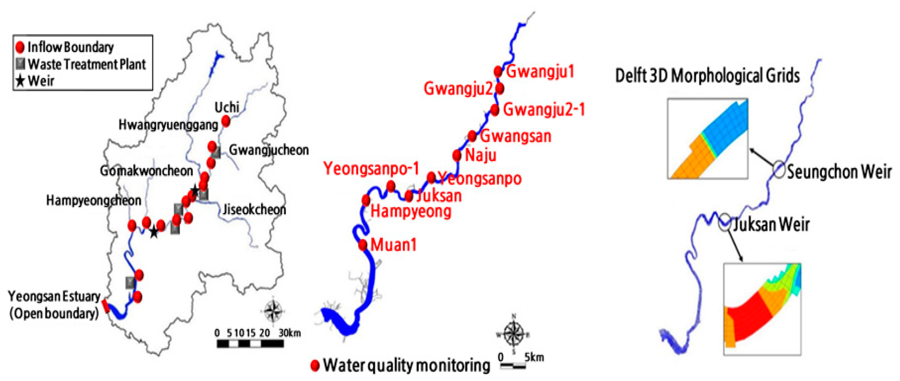
In this study, the Delft3D model was configured for a 103 km section of the mainstream of the Yeongsan River (see Figure 1). Orthogonal–curvilinear grids were employed, with a total of 2626 grid cells. The horizontal grid size ranged from 47 to 315 m, with a lateral average of 145 m and a longitudinal average of 113 m. The vertical direction of the grid used a σ-coordinate system, composed of five equally spaced water columns. Surface elevation data from the Korea Institute of Civil Engineering and Building Technology (KICT) [28] were utilized for all grids.
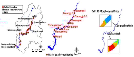
Figure 1.
The study area, with information on inflow boundaries and contour grids.
In terms of inflow boundary conditions, a total of 20 different conditions were defined, encompassing 13 tributaries (e.g., the Hwangryong River, Jiseok Stream, and Gwangju Stream) and effluents from six public wastewater treatment plants (WTPs) (e.g., Gwangju, Damyang, and Naju). For meteorological boundary conditions, hourly data from the Korea Meteorological Administration (KMA) were incorporated, including temperature, precipitation, and cloud cover, and for specific regions, data from the Gwangju and Mokpo weather stations were used [29].
Of the inflow boundary conditions, weekly flow data were obtained from the Water Environment Information System (WEIS) of the National Institute of Environmental Research, while daily data were sourced from the Yeongsan River Flood Control Office of the Water Resources Management Information System (WAMIS). Water quality data were extracted from the National Automatic Water Quality Monitoring System of the Ministry of Environment, and for effluent data from wastewater treatment plants (WTPs), daily monitoring data released by the respective agencies were used in model construction [30,31]. Additionally, for the boundary conditions at the downstream ends of the river, daily water level data from the Yeongsan River Barrage, provided by the Yeongsan River Flood Control Office, were applied.
As for the BLOOM model, it differs from conventional models based on the Monod type in that it considers changes in the carbon/nitrogen (C/N) ratio of algae based on real natural environmental conditions. This allows for the determination of the dynamic variation of physiological–ecological characteristics of algae. By considering the competition between different algal species/types and their adaptations to environmental changes, the model enables the simulation of a decrease in the C/N ratio of algae under conditions of nitrogen limitation and an increase in the ratio under conditions of light limitation.
2.2. Monitoring Data
In this study, HABITAT 3.0 (Deltares, Delft, The Netherlands), a spatial analysis tool specifically designed for ecological assessment, was employed to analyze changes in the habitat suitability of target fish species. Surfer 16 (Golden Software, Golden, CO, USA), a 3D data visualization and mapping software application, was used for the conversion and application of the grids generated in the Delft3D model. The simulation results from the Delft3D-FLOW module and the Delft3D-WAQ module were utilized for the assessment of physical and chemical changes, respectively. For the HABITAT model, input data included Habitat Suitability Curves (HSCs) based on physical and chemical parameters for each target species.
For the target fish species, data from projects linked with the basic environmental survey program and monitoring in the Yeongsan River were utilized [20,21,22]. Seventeen fish species, including dominant and endemic species, were selected for the study: Squalidus chankaensis tsuchigae, S. variegatus wakiyae, Z. platypus, H. labeo, P. esocinus, C. auratus, L. macrochirus, C. carpio, A. koreensis, H. eigenmanni, M. salmoides, A. macropterus, striped shiner, S. czerskii, M. yaluensis, N. koreanus, and P. altivelis. In the HABITAT model, these species were represented using Habitat Suitability Curves (HSCs) for physical and chemical parameters. These curves were constructed by applying the Instream Flow and Aquatic Systems Group I (FASG) method, first proposed by Gosse [32].
2.3. Methods
2.3.1. Hydraulic Simulation
The Delft3D model is a comprehensive 3D modeling suite developed by Deltares, an independent Dutch institute for applied research. It is capable of numerical simulation for flows, including sediment transport and water quality changes in freshwater, estuaries, and marine water bodies. The model is versatile, enabling the selection of different modules (hydraulics, sediment transport, water quality, and algae) for linking and applications based on specific research objectives. Within the Delft3D-FLOW module, four options for numerical analysis are available: stability analysis, implicit–explicit methods, error rate reduction, and simulations of rapid fluctuations. The advection term can be calculated by selectively combining and applying these options. The FLOW module performs a numerical analysis of hydrodynamics and consists of 3D nonlinear continuity equations and shallow water equations. The governing equation, based on the Boussinesq assumption of incompressible fluid, is presented as follows.
<Continuity equation>
where t indicates time; ξ and η denote horizontal axes (spherical coordinate system); Q is the flow rate (m3/s); ζ is the water depth above the reference level (datum level) (m); d is the water depth below the reference level (m); and U and V represent mean flow velocity (m/s) in the ξ and η directions, respectively. In the Delft3D model, flow velocity in the vertical direction can be computed by the continuity equation, and momentum equations in the horizontal (ξ) and perpendicular (η) directions are shown below.
<Momentum equations>
where ω denotes flow velocity in the vertical direction (m/s); f represents the Coriolis constant (1/s); ρ0 indicates density of seawater (kg/m3); ν is the kinematic viscosity (m2/s); Pξ and Pη are pressure gradients in ξ and η directions; Fξ and Fη are the imbalance of Reynolds stress in ξ directions (m2/s); and Mξ and Mη represent generated and dissipated momentums, respectively. In addition, the state equation (density), hydrostatic pressure conditions, and turbulence terms are included to constitute basic equations included in the Delft3D-FLOW module.
2.3.2. Water Quality Simulation
Delft3D-WAQ is a module designed for the numerical simulation of water quality. It is applied in conjunction with flow field information obtained through hydraulic analysis. The WAQ module facilitates the simulation of the dynamics of dissolved oxygen, nutrients, and organic matter through an extensive range of reaction networks involving organic matter, such as mineralization, settlement and resuspension, nitrification, and denitrification.
<Mass balance equation>
where C represents the concentration of water quality variable; u, v, and w indicate flow velocity components in the x, y, and z coordinates, respectively; Kx, Ky, and Kz represent the turbulent diffusion coefficients (x, y, and z coordinates); and Sc represents the external and internal source and sink terms. In the Delft3D-WAQ module, the basic modeling equation shares similarities with the equation for thermohaline circulation. In addition to this, the internal source and sink terms of biogeochemical cycles may be incorporated to represent the model. The module also allows for the consideration of hydrodynamic responses for a total of 32 ecological variables related to water quality. This flexibility permits the accounting of source/sink processes and interactions between variables for each water quality variable. In this study, to address interactions between variables for external and internal source and sink terms, we introduced empirical formulae for heat exchange across the air–water interface, nitrification, denitrification, and oxygen consumption. These additions were made to the basic composition of the dissolved oxygen (DO)–biochemical oxygen demand (BOD) model. Further details on a range of empirical formulae for water-quality-modeling items and equations governing relationships between variables through the source and sink processes for each applicable water quality variable can be found in Deltares [33].
2.3.3. Bloom Simulation
The Delft3D-BLOOM module allows for the simulation of competition between various algal species and types, considering species adaptation to limiting factors and changes in the number of individuals due to extinction. The application of the Delft3D model with these different modules has been reported in numerous previous studies [34,35,36].
With the Delft3D-BLOOM module, the characteristics of the aquatic environment, with complex spatiotemporal variabilities, can be considered. It can selectively simulate a total of 21 algal species, and N (physiological characteristics of species in the case of nitrogen limitation), P (physiological characteristics of species in the case of phosphorus limitation), and E (physiological characteristics of species in the case of light limitation) can be applied based on environmental conditions.
Rather than adjusting specific coefficients for the reproduction of temporary and local conditions in the aquatic environment, the model coefficients are determined with a balance in the overall calculation process to derive the optimal combination of coefficients. The equation of mass conservation for algae can be expressed as follows.
Algae undergo various processes, including gross primary production, respiration, excretion, mortality, grazing, resuspension, and settling. Net growth (increase in biomass) is the result of these influencing factors. Net primary production is defined as the value obtained by subtracting respiration from gross primary production. The BLOOM module simulates the remaining responses, excluding excretion, grazing, resuspension, and settling. The grazing, resuspension, and settling of algae are calculated in the WAQ module, which models physical processes such as advection–diffusion and external load within the same structure. Algal biomass is converted into inorganic nutrients or organic detritus in water columns. Settled algae will die and decompose immediately or gradually, depending on conditions, and are converted into organic detritus in sediments. Predation can be considered if the grazing module is activated in the WAQ module. Predation can be simulated either by artificially setting predation pressure or by simulating the dynamics of predatory zooplankton. Other responses are similar to existing models, but the primary production is estimated by combining the same deterministic concept of existing models with mathematical solutions. In most cases, existing models calculate the growth rate (production rate) using a multiplicative formulation that comprehensively considers the constraints of light, water temperature, and nutrients in the maximum growth rate. At this time, for nutrient constraints, a minimum formulation is applied, considering only the minimal limiting factors among N, P, and Si (for diatoms).
where Px denotes growth rate; PMx represents the maximum growth rate; N, I, and T indicate nitrogen (N), light intensity, and temperature, respectively; DIN, PO4, and Si denote concentrations of dissolved inorganic nitrogen, phosphate, and silicate, respectively; f1(N), f1(I), and f1(T) represent minimum limiting factors according to N, light intensity, and temperature, respectively; and KHN, KHP, and KHS indicate the half-saturation constant of the nutrients N, P, and Si, respectively. In comparison with the above equation, BLOOM introduces the concept of competition and adaptation in algal species to calculate the growth rate by mathematically finding the solution with the small resource demand required for survival and maximum growth rate.
where Pnx,i denotes the unit growth rate of algae (x, i), and Nx,i represents the resource demands (light, nutrients, N-P-Si) of algae (x, i).
2.3.4. Habitat Simulation
The ecological assessment model can be categorized into data-based analysis and habitat suitability based on field monitoring. These two different approaches can be selected based on the research objectives and conditions under consideration. An ecological assessment model compatible with the Delft3D model is the HABITAT model developed by Deltares in the Netherlands. The HABITAT model serves as a spatiotemporal analysis tool for assessing a diverse range of plans not only in the aquatic environment but also within the watershed. The advantages of the HABITAT model include its requirement for a small amount of input data, its ability to run in connection with various hydraulics and water quality analysis results, and the rapid detection of habitable areas based on the habitat suitability of the target species. However, a challenge lies in obtaining habitat suitability data for the target species, as this often requires referencing data from previous studies or foreign literature. To address this limitation, Deltares offers Habitat Suitability Curves (HSCs) for basic habitat conditions and related information for several major target species in the ecosystem, free of charge.
The HABITAT model’s analysis module comprises four types: broken linear reclassification model, formula-based calculation model, classification model (single), and classification model (multiple). The selection of a module depends on the dependent and independent variables in the analysis. Generally, a broken linear model or a formula-based calculation model is used for analysis. These various modules provide results that serve as fundamental data for analyzing and interpreting the causal relationships between indicator species, community species, and habitat types in relation to specific environmental conditions. While it is possible to use the HABITAT model with the habitat data for various organisms provided by Deltares, adapting the model to the environmental conditions of South Korea requires collecting and monitoring data that offer quantitative information on the relationship between environmental factors and the habitat suitability (response curve) of various species. These data should be organized into a database for the continuous utilization of the HABITAT model in various fields in South Korea. An ecological-knowledge-based approach is essential in designing the model to ensure its effective and continuous application.
2.3.5. Methods of Model Reproducibility Assessment and Scenario Development
In this study, to assess the reproducibility of the Delft3D model, calibration was conducted for the period from 1 January to 31 December 2019, while model validation was performed from 1 January to 31 December 2020. Various indicators were employed to analyze reproducibility, including Nash–Sutcliffe efficiency (NSE), percent bias (PBIAS), bias, index of agreement (IOA), and mean absolute error (MAE). NSE was used to evaluate the predictive skills of the model, while bias and PBIAS served as indicators of the average trend of the simulated data. Additionally, MAE and IOA were applied as indicators to analyze prediction accuracy between the simulated and observed data. These indicators are defined as follows.
where Pi denotes the simulated value (at time i), Oi denotes the observed value (at time i), and Ōi denotes the mean of the observed values over the total period of observation.
2.3.6. Scenarios of Weir Operations
To investigate the effects of hydraulic structure operation on changes in habitat suitability, we developed simulation conditions (scenarios). For the Seungchon weir and the Juksan weir, which were already installed in the mainstream of the Yeongsan River, the following scenarios were developed based on the assumption that a set water level would be maintained through the opening of sluice gates, according to recent weir-opening conditions:
- (Condition 1) Seungchon weir partial opening (elevation: 6.0 m)—Juksan weir, full opening (elevation: −1.35 m, lowest water level)
- (Condition 2) Seungchon Weir full opening (elevation: approximately 2.7 m)—Juksan weir partial opening (mean water level elevation: 1.5 m)
2.3.7. AI Methods for Predicting Chl-a Concentrations
In this study, we employed artificial intelligence models, specifically, recurrent neural network (RNN) and long short-term memory (LSTM) network, to predict Chl-a concentrations based on a diverse set of input variables. The neural network architecture consisted of eight hidden layers, each comprising 50 to 100 nodes. Regarding the input variables, we conducted correlation analysis to identify the variables with the highest correlation. Two scenarios were explored: one where only variables with the highest correlation were selectively applied and another where all variables were included. The prediction results were then derived for each scenario.
3. Results and Discussions
3.1. Delft3D-FLOW Model
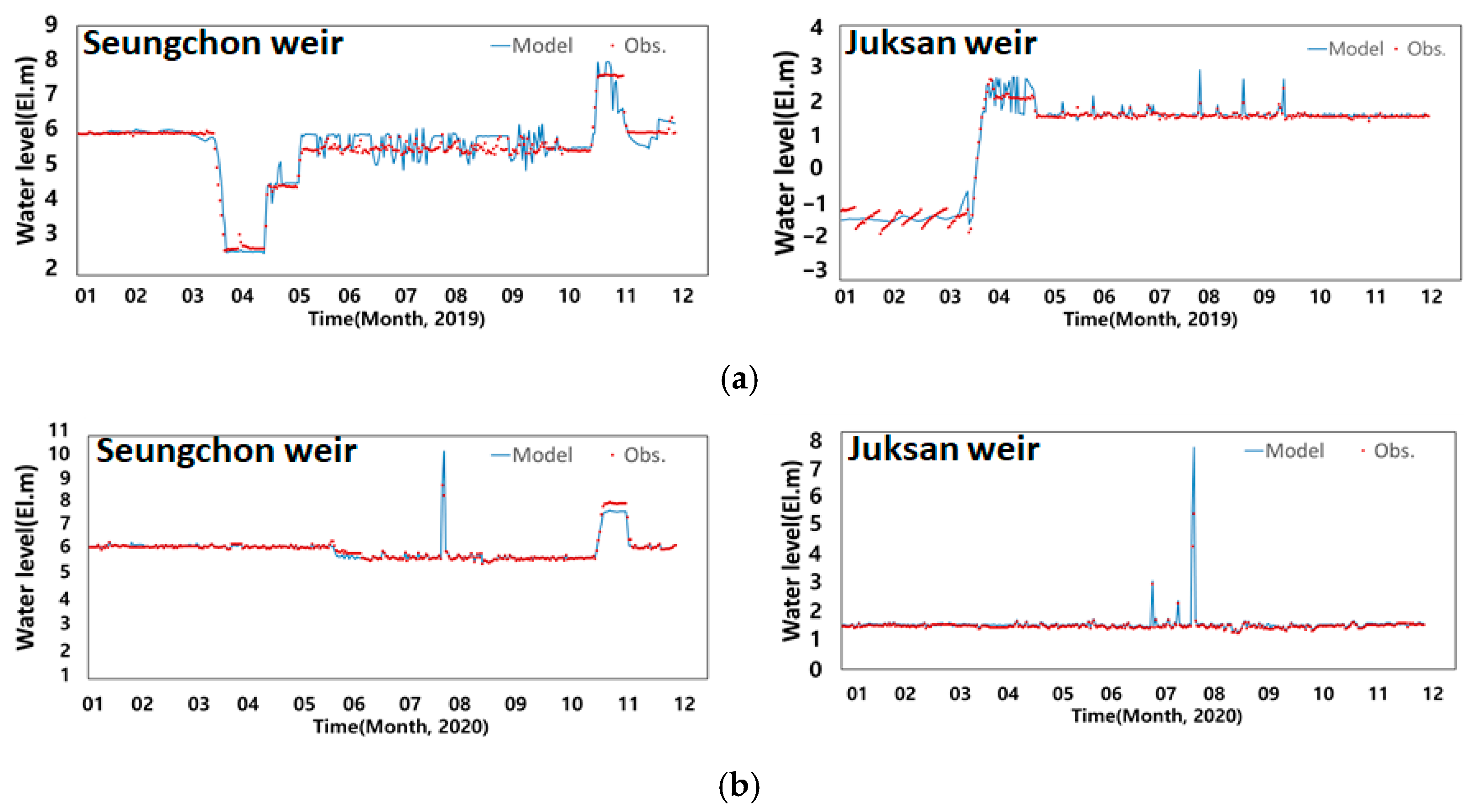
The Delft3D-FLOW module was utilized to assess the reproducibility of water levels at the Seungchon and Juksan weirs on the Yeongsan River. Comparing the simulated and measured values, the results indicated close agreement, as demonstrated by the following indicators: bias ranging from −0.08 to 0.35 m, MAE from 0.26 to 0.33 m, NSE from −2.05 to 0.96, PBIAS from −1.58 to 4.41%, and IOA from 0.84 to 0.98 (see Figure 2 and Table 1). The comparison of simulated values obtained using the Delft3D-FLOW module with the measured values of the Yeongsan River revealed a strong performance, accurately predicting the overall trend of the data. Additionally, applying the accuracy evaluation method proposed by Moriasi et al. [37] resulted in high ratings, ranging from “satisfactory” to “very good” based on the criteria.
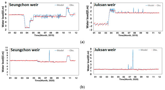
Figure 2.
Comparison of simulated and observed water levels of Seungchon (left) and Juksan (right) weirs. (a) Model Calibration. (b) Model Verification.

Table 1.
Statistical results for the error index based on simulated water level and water quality results.
3.2. Deft3D-WAQ-BLOOM Model
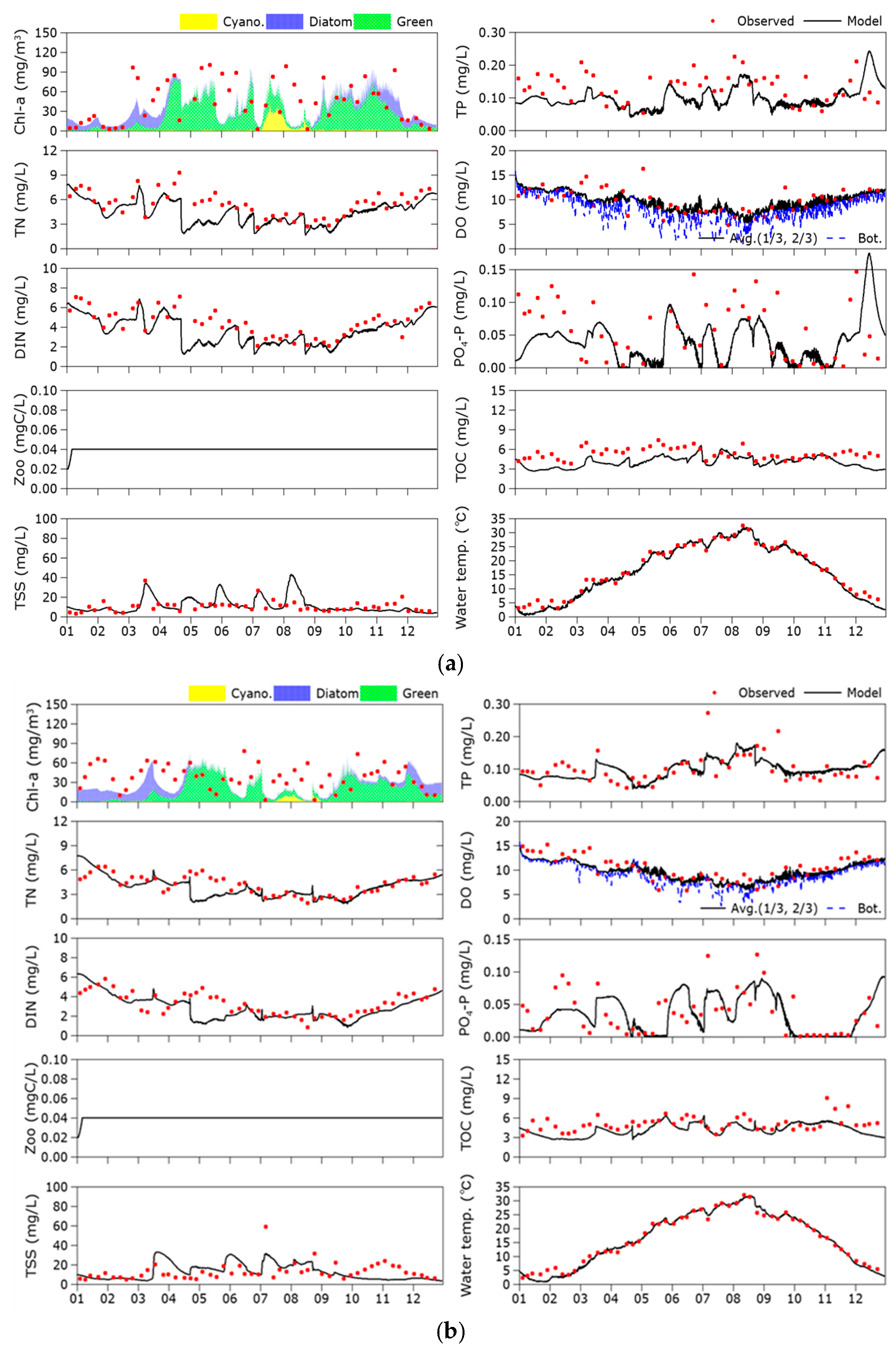
To assess the reproducibility of water quality modeling using the Delft3D-WAQ-BLOOM module, we conducted comparisons between simulated and measured values for nine items, including water temperature, dissolved oxygen (DO), total nitrogen (T-N), and total phosphorus (T-P), at representative locations near the Seungchon and Juksan weirs in the Yeongsan River (refer to Figure 3). In the Delft3D-WAQ module, we applied appropriate coefficient values within the specified characteristics and range for water quality parameters (see Table 2). For the Delft3D-BLOOM module, we used the characteristics and applied values of coefficients for each type of algae, as outlined in Table 3 and Table 4.
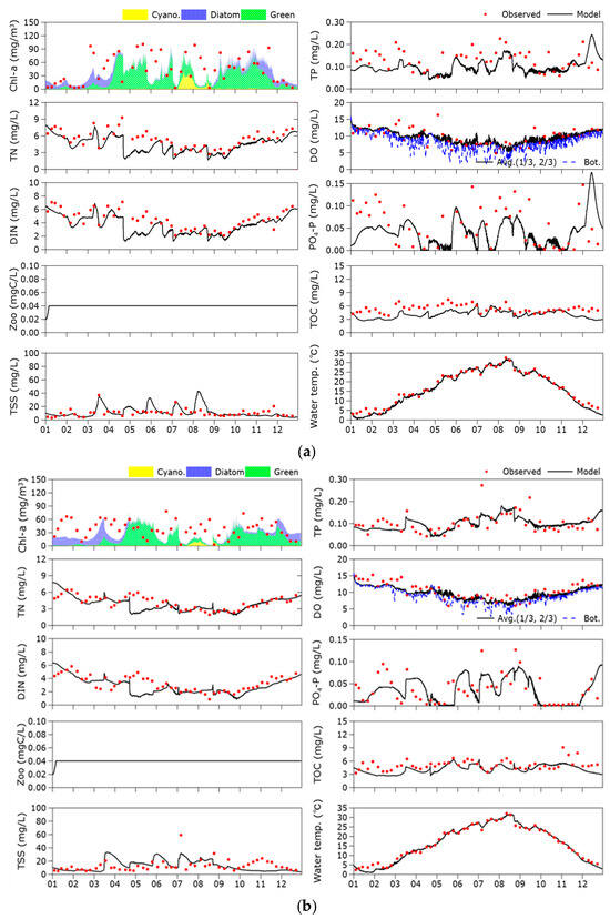
Figure 3.
Comparison of simulated and observed water quality. (a) Seungchon weir. (b) Juksan weir.
Table 2.
The water quality parameter information in the simulation.
Table 3.
The parameters of the Delft3D-BLOOM model in the simulation [38].
Table 4.
The coefficients of growth, mortality, and respiration [39].
The resulting indicators for the comparisons were as follows: bias, −1.42 to 0.56 mg/L; MAE, 0.46 to 0.71 mg/L; NSE, 0.68 to 0.94; PBIAS, −1.85 to 0.91%; and IOA, 0.62 to 0.96 (see Table 1). Specifically, for water temperature comparisons, the indicators were bias, −0.25 to 0.02 °C; MAE, 0.11 to 0.15 °C; NSE, 0.91 to 0.95; PBIAS, 0.05 to 2.24%; and IOA, 0.88 to 0.97.
When comparing simulated values using the integrated Delft3D-WAQ-BLOOM model for the Yeongsan River with measured values, the model demonstrated good overall performance in predicting trends. However, it either underestimated or overestimated some data with significant variability.
In the period from January to March, concentrations of T-N and DIN derived from the model were underestimated, likely because of low mainstream flow and the significant impact of point sources such as the Gwangju WTP. After April, the simulated values aligned well with the measured values. High concentrations of T-P and PO4-P from March to August were attributed to nonpoint sources like watershed runoff, leading to model underestimation. From January to May, simulated TOC concentration values were lower than the measured values, potentially because of the underestimation of particulate organic carbon in tributaries.
This study underscores the importance of calibrating and validating the model, especially in situations with large data variability or outliers. The improved optimization of coefficients is necessary, utilizing data from diverse water quality monitoring networks to recalibrate the model and accurately reflect the characteristics of rivers and streams in South Korea.
3.3. Prediction of Changes in Aquatic Ecosystems with Environmental Changes
3.3.1. Analysis of Changes in Algae with the Delft3D-BLOOM Module
In the Delft3D-BLOOM module, the calculation of the rate of change in algae involves considering available resources from specific times and locations, including biomass and algal types. Conditions related to light energy, growth, mortality, and nutrients were reconstructed and then applied to the model. This approach allowed for the examination of changes in algae based on ecological–physiological conditions, such as succession through the competition of algal species and adaptation to environmental changes.
3.3.2. Changes in Biological Life Cycle by Algal Type
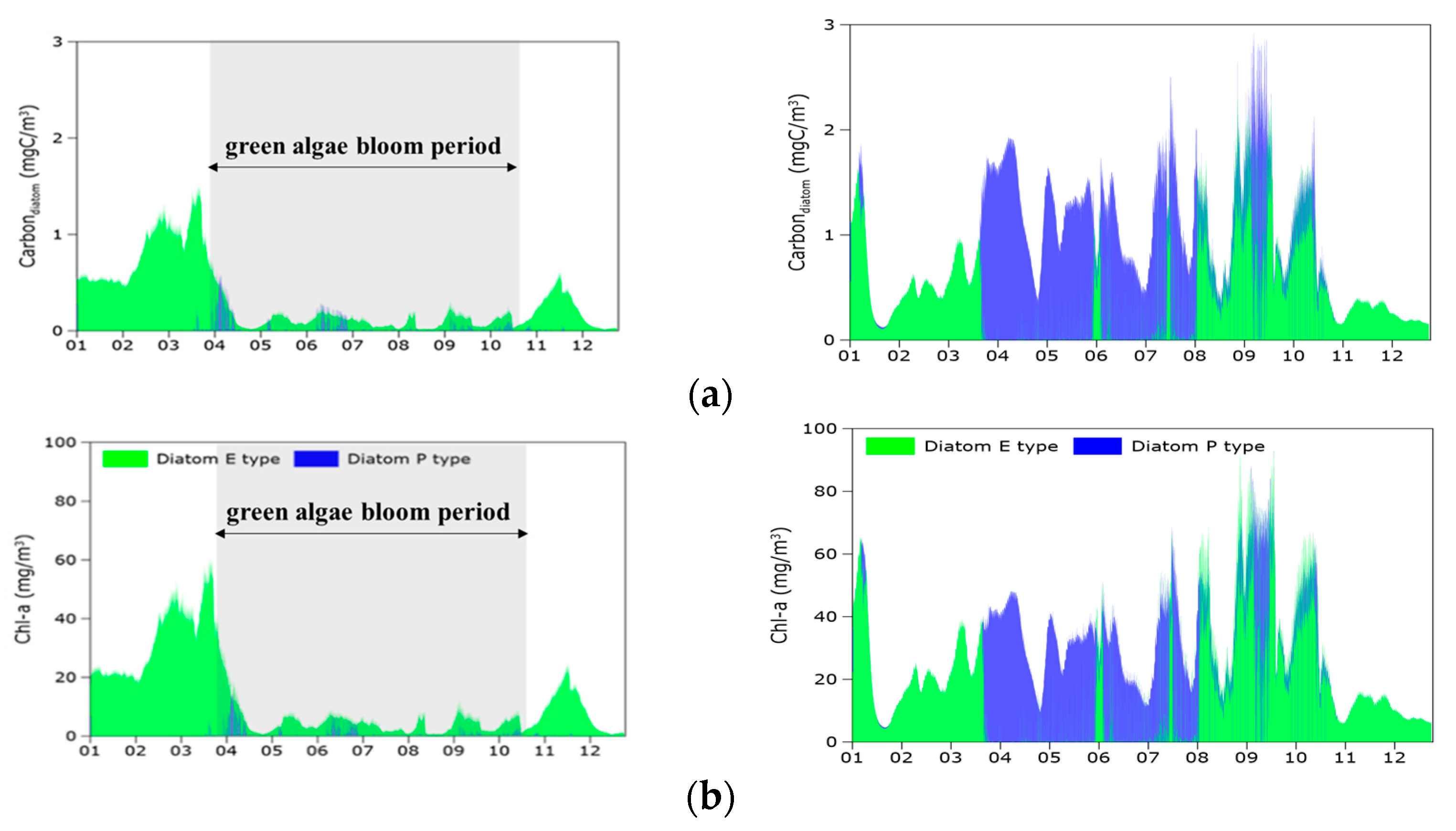
Figure 4 illustrates the temporal changes in algae at the Seungchon and Juksan weirs considering competition between algal species, adaptation, and succession. In general, diatoms dominate during winter when the water temperature is low. As the water temperature increases, the algal composition shifts, with green algae becoming dominant. To provide more detail, from the end of February to the beginning of March, a brief period of phosphorus limitation occurs because of low flow/the dry season and agricultural off-season conditions. During this time, both P-type diatoms and green algae exhibit dominance. However, during the wet season, there is a sharp decrease in Chl-a concentrations due to flushing phenomena. Following the wet season and without light limitation, the amount of E-type algae experiences a rapid increase.
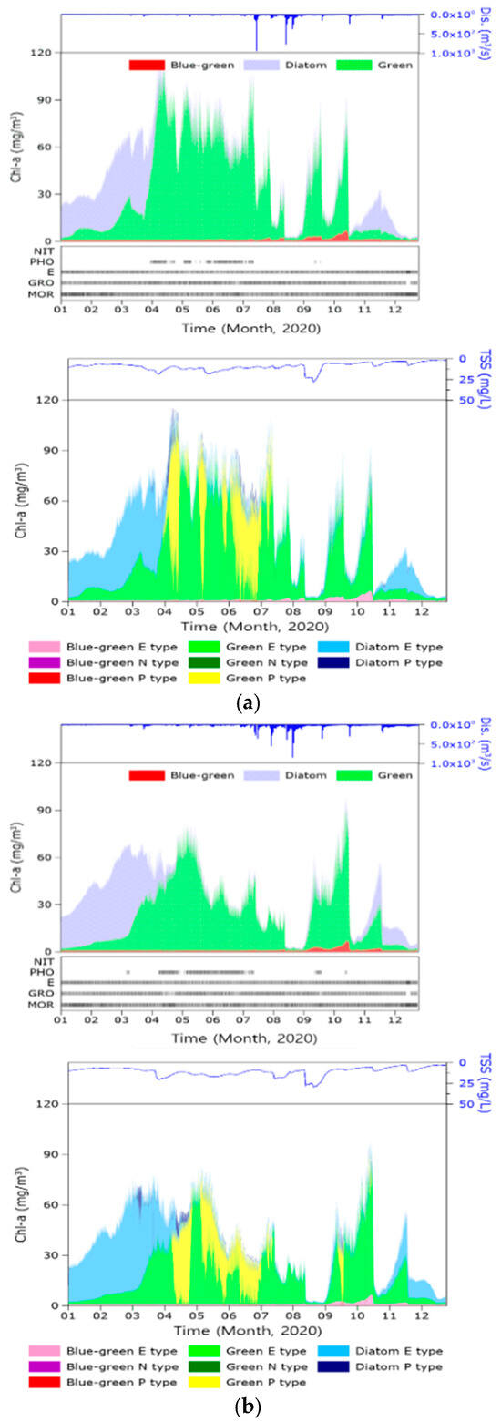
Figure 4.
Changes in the life stages of algae. (a) Seungchon weir. (b) Juksan weir.
3.3.3. Adaptation and Succession of Algae According to Weir Operation Scenarios
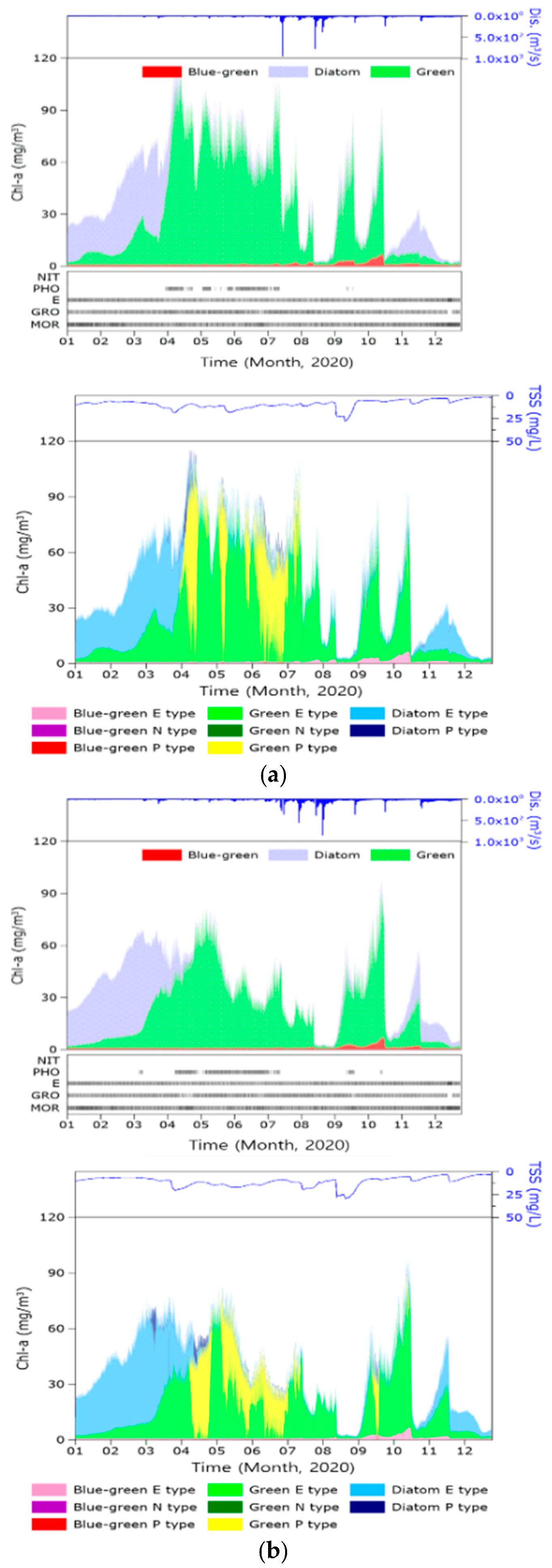
Figure 5 depicts variations in algae based on different weir operation scenarios. The rapid adaptation of algae to swiftly changing environmental conditions is evident, particularly in response to phosphorus limitation and the full opening of the weir. Specifically, when the sluice gates of the weir remain closed, green algae tend to dominate from April onward as the water temperature rises. In contrast, with fully opened sluice gates, diatoms become the dominant species during the period when green algae would typically prevail. The prevalence of diatoms signifies an abundant food source for zooplankton, which, in turn, serves as a food source for fish. Consequently, in the long term, this shift is anticipated to contribute to the improvement of aquatic ecosystem health in this area.
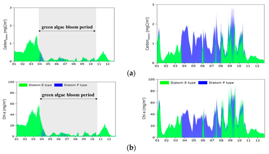
Figure 5.
Changes in algae in weir operation scenarios. (a) Seungchon weir. (b) Juksan weir.
3.3.4. Prediction of Changes in Algae with Artificial Intelligence Models
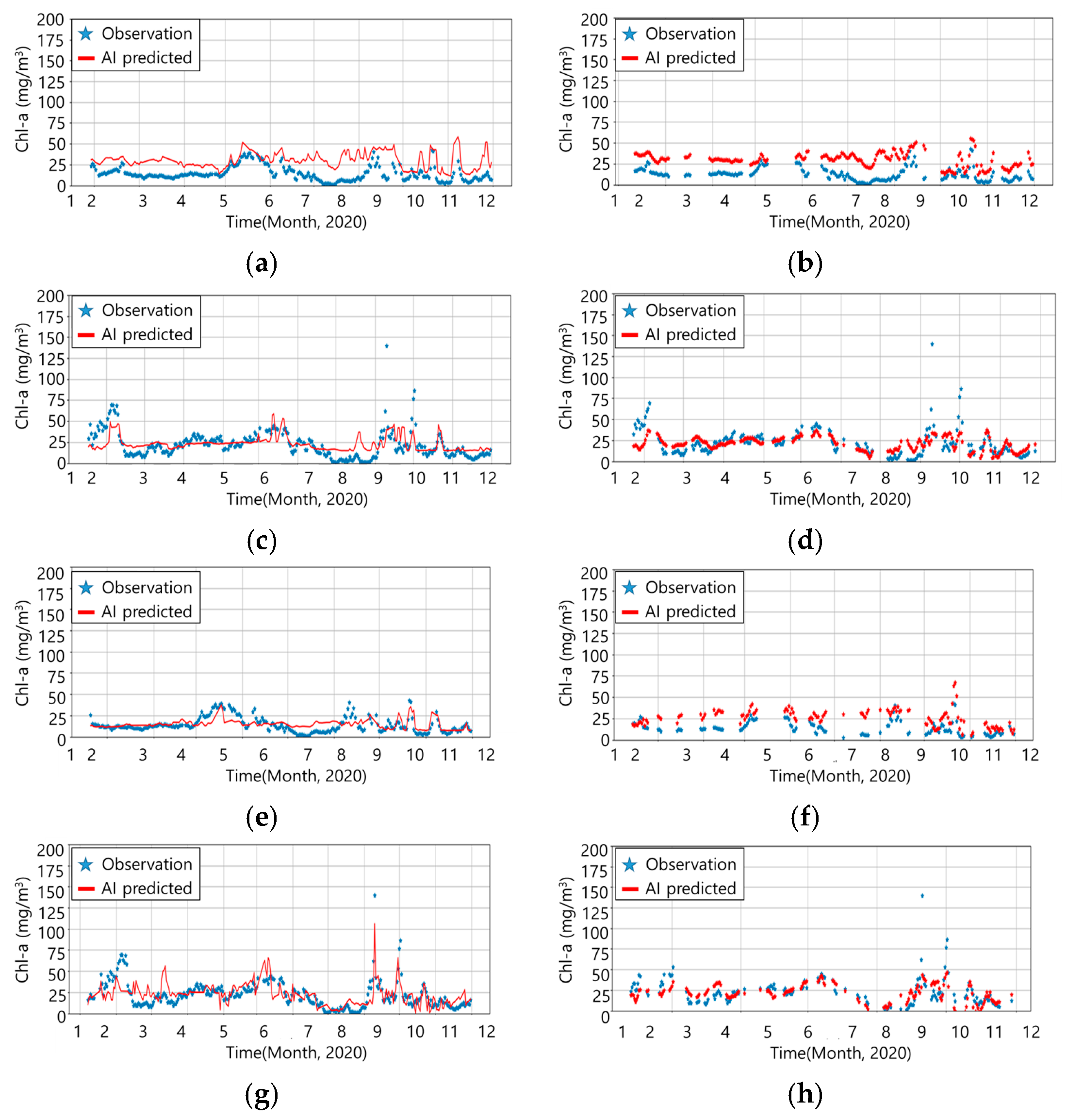
To predict hydraulics–water quality and aquatic ecology, deterministic models like the Delft3D model are often employed. These models analyze changes in parameters in response to environmental shifts. However, performing numerical simulations with such models requires a substantial amount of input data, computational resources, and expertise, creating barriers to method accessibility. In recent years, the emergence of AI models has provided an alternative. These models offer quick predictions and are more user-friendly compared with numerical simulations, making them particularly useful for short-term predictions. AI models learn patterns from past events and make predictions based on these learned patterns. Prediction accuracy improves with the accumulation of data over time. The LSTM model, in particular, demonstrated superior prediction accuracy compared with RNN. Additionally, even when the correlation between predictive variables and input variables was low, including data from numerous variables enhanced the prediction accuracy of the AI models, outperforming the application of selective variables (refer to Table 5 and Figure 6).
Table 5.
The accuracy of each case according to input and output factors.
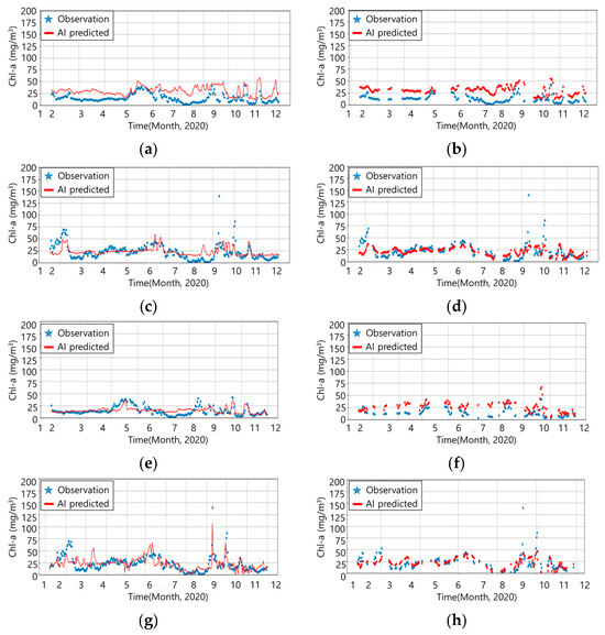
Figure 6.
Comparison of simulated and measured results from AI methods. (a) Case 1. (b) Case 2. (c) Case 3. (d) Case 4. (e) Case 5. (f) Case 6. (g) Case 7. (h) Case 8.
3.3.5. Prediction of Changes in Aquatic Ecosystem Health Index through the Integrated Delft3D-HABITAT Model
In Figure 7, an integrated model coupling the results of hydraulic analysis from the Delft3D model with the HABITAT model was developed. This integrated model was then used to predict changes in the aquatic ecosystem health index of the Yeongsan River. The prediction of the aquatic ecosystem health index involved aggregating habitat changes for 17 fish species inhabiting the Yeongsan River. The habitat area was categorized into levels based on various weir operation scenarios. To evaluate these levels, the Hydraulic Habitat Suitability (HHS) index, as described by Zingraff-Hamed et al. [40], was employed. The rating criteria considered the ratio of the area occupied by the 17 fish species to the total area of the modeled section of the Yeongsan River. The habitat area was divided into five levels, and the criteria for each level are presented as follows:
- (Very high) HHS index > 80%
- (High) 50% < HHS index < 80%
- (Medium) 30% < HHS index < 50%
- (Low) 10% < HHS index < 30%
- (Very low) HHS index < 10%
The changes in the aquatic ecosystem health index were assessed under two different scenarios. This index is determined by dividing the sum of the inhabitable area of the target species by the total study reach area. In the application of each scenario, the index saw an improvement. Specifically, in scenario 1, it increased by one level from low to medium, while in scenario 2, it rose from medium to high. This suggests that keeping the sluice gate of the Seungchon weir fully open optimizes the aquatic ecosystem health index. Notably, the results indicated that the improvement was most significant when the sluice gate of the Seungchon weir was fully opened. However, in the case of the Juksan weir, the increase in the ecosystem health index was relatively modest, likely because of the presence of a stagnant body of water downstream of the barrage. Additionally, considering the fish species in the Yeongsan River, those associated with lotic habitats were observed more frequently than those linked to lentic habitats.
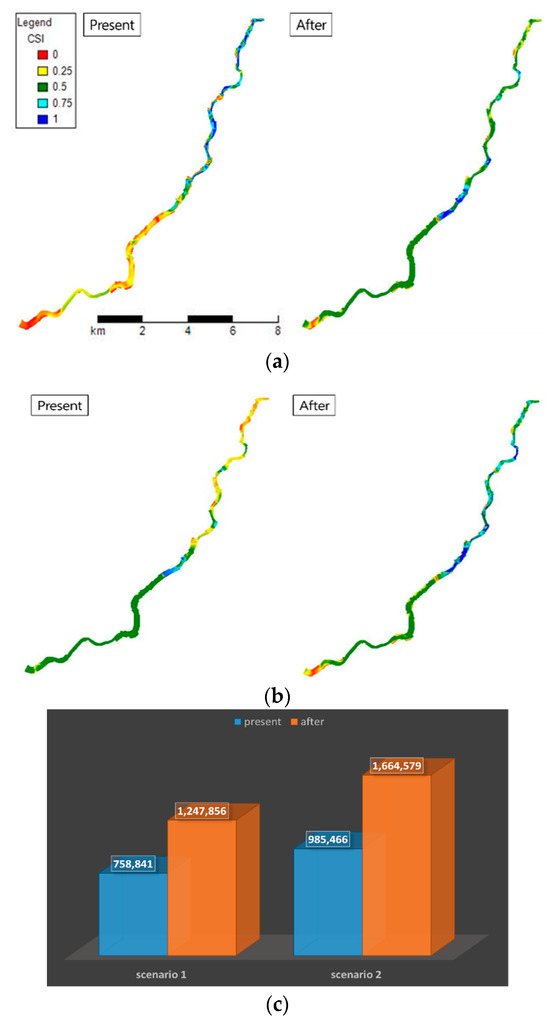
Figure 7.
Changes in aquatic ecosystem health in weir operation scenarios. (a) Scenario 1. (b) Scenario 2. (c) Changes in habitat area in weir operation scenarios.
Figure 7.
Changes in aquatic ecosystem health in weir operation scenarios. (a) Scenario 1. (b) Scenario 2. (c) Changes in habitat area in weir operation scenarios.

4. Conclusions
This study focused on the global shift toward emphasizing environmental conservation and sustainable ecosystem management. It involved the development of an integrated modeling framework for the Yeongsan River, enabling the analysis of physical, chemical, and ecological factors to predict habitat changes in various environmental scenarios. The objective was to suggest management strategies for improving the health of the aquatic ecosystem.
This study commenced with the establishment of a Delft3D model for the Yeongsan River, assessing its reproducibility concerning water level and quality. The BLOOM module within Delft3D was employed to analyze algae dynamics and their responses to environmental changes, revealing a transition from diatom to green algae dominance with the complete opening of weir gates, which could potentially enhance the aquatic ecosystem.
Using a HABITAT model informed by data on 17 fish species, this study predicted changes in aquatic habitats in response to various weir operation scenarios. The results indicate that the aquatic ecosystem’s health improves significantly with the full opening of at least one weir gate.
Furthermore, an AI model, specifically an LSTM network, predicted changes in algae more accurately when all input variables were utilized. This integrated prediction model, which combines Delft3D and HABITAT, can serve as a valuable tool for integrated water resource management. It assesses the effects of physical and chemical environmental changes in aquatic ecosystems, enabling the evaluation of improvements in hydraulics, water quality, and aquatic ecology in alignment with the evolving paradigm of aquatic ecosystem management.
Author Contributions
Conceptualization, B.C., W.-S.L. and E.N.; Methodology, B.C., J.P. and T.-W.K.; Validation, J.P., T.-W.K., W.-S.L. and E.N.; Formal analysis, B.C., D.-W.H., S.-Y.H. and J.C.; Investigation, B.C., D.-W.H., S.-Y.H. and J.C.; Writing—original draft, B.C.; Writing—review & editing, B.C., J.C.; Supervision, J.P., T.-W.K., W.-S.L. and E.N.; Project administration, W.-S.L. All authors have read and agreed to the published version of the manuscript.
Funding
This research was supported by a grant (NIER-2022-01-01-044) from the National Institute of Environmental Research. In addition, this paper is part of a NIER research report (Report Name: “Application of habitat analysis and modelling for improvement of aquatic ecosystem health in the Yeongsan River (III)”).
Institutional Review Board Statement
Not applicable.
Informed Consent Statement
Not applicable.
Data Availability Statement
The data presented in this study are available on request from the corresponding author.
Acknowledgments
The authors appreciate the suggestions and enthusiastic support of the editors and reviewers.
Conflicts of Interest
The authors declare no conflict of interest.
References
- Lee, M.; Kim, H.; Lee, J.Y. A Shift Towards Integrated and Adaptive Water Management in South Korea: Building Resilience Against Climate Change. Water Resour. Manag. 2022, 36, 1611–1625. [Google Scholar] [CrossRef]
- Sadat, M.A.; Guan, Y.; Zhang, D.; Shao, G.; Cheng, X.; Yang, Y. The associations between river health and water resources management lead to the assessment of river state. Ecol. Indic. 2020, 109, 105814. [Google Scholar] [CrossRef]
- Ministry of Environment (MOE). The First National Water Management Plan (2021–2030); Ministry of Environment: Sejong, Republic of Korea, 2020. [Google Scholar]
- Ministry of Environment (MOE). The Second National Water Environment Management Master Plan; Ministry of Environment: Sejong, Republic of Korea, 2015. [Google Scholar]
- Bovee, K.D. A Guide to Stream Habitat Analysis Using the Instream Flow Incremental Methodology; Western Energy and Land Use Team, Office of Biological Services, Fish and Wildlife Service, US Department of the Interior: Washingtown, DC, USA, 1982. [Google Scholar]
- Wasson, J.; Tusseau-vuillemin, M.; Andréassian, V.; Perrin, C.; Faure, J.; Barreteau, O.; Bousquet, M.; Chastan, B. What kind of water models are needed for the implementation of the European Water Framework Directive? Examples from France. Int. J. River Basin Manag. 2003, 1, 125–135. [Google Scholar] [CrossRef]
- Valentin, S.; Lauters, F.; Sabaton, C.; Breil, P.; Souchon, Y. Modelling temporal variations of physical habitat for brown trout (Salmo trutta) in hydropeaking conditions. Regul. Rivers Res. Manag. 1996, 12, 317–330. [Google Scholar] [CrossRef]
- Tharme, R.E. A global perspective on environmental flow assessment: Emerging trends in the development and application of environmental flow methodologies for rivers. River Res. Appl. 2003, 19, 397–441. [Google Scholar] [CrossRef]
- Booker, D.J.; Dunbar, M.J.; Ibbotson, A. Predicting juvenile salmonid drift-feeding habitat quality using a three-dimensional hydraulic-bioenergetic model. Ecol. Model. 2004, 177, 157–177. [Google Scholar] [CrossRef]
- Colosimo, M.F.; Wilcock, P.R. Alluvial sedimentation and erosion in an urbanizing watershed, Gwynns Falls, Maryland. J. Am. Water Resour. Assoc. 2007, 43, 499–521. [Google Scholar] [CrossRef]
- García, A.; Jorde, K.; Habit, E.; Caamaño, D.; Parra, O. Downstream environmental effects of dam operations: Changes in habitat quality for native fish species. River Res. Appl. 2011, 27, 312–327. [Google Scholar] [CrossRef]
- Papadaki, C.; Ntoanidis, L.; Zogaris, S.; Martinez-Capel, F.; Muñoz-Mas, R.; Evelpidou, N.; Dimitriou, E. Habitat hydraulic modelling for environmental flow restoration in upland streams in Greece. In Proceedings of the 12th International Conference on Protection and Restoration of the Environment, Skiathos Island, Greece, 29 June–3 July 2014. [Google Scholar]
- Chen, Q.; Zhang, X.; Chen, Y.; Li, Q.; Qiu, L.; Liu, M. Downstream effects of a hydropeaking dam on ecohydrological conditions at subdaily to monthly time scales. Ecol. Eng. 2015, 77, 40–50. [Google Scholar] [CrossRef]
- Bunn, S.E.; Arthington, A.H. Basic principles and ecological consequences of altered flow regimes for aquatic biodiversity. Environ. Manag. 2002, 30, 492–507. [Google Scholar] [CrossRef] [PubMed]
- Choi, B.; Choi, S.U. Physical habitat simulations of the Dal River in Korea using the GEP Model. Ecol. Eng. 2015, 83, 456–465. [Google Scholar] [CrossRef]
- Nikghalb, S.; Shokoohi, A.; Singh, V.P.; Yu, R. Ecological regime versus minimum environmental flow: Comparison of results for a river in a semi Mediterranean region. Water Resour. Manag. 2016, 30, 4969–4984. [Google Scholar] [CrossRef]
- Im, D.; Choi, S.U.; Choi, B. Physical habitat simulation for a fish community using the ANFIS method. Ecol. Inform. 2018, 43, 73–83. [Google Scholar] [CrossRef]
- Choi, S.U.; Kim, S.K.; Choi, B.; Kim, Y. Impact of hydropeaking on downstream fish habitat at the Goesan Dam in Korea. Ecohydrology 2017, 10, e1861. [Google Scholar] [CrossRef]
- Gard, M. Modeling changes in salmon spawning and rearing habitat associated with river channel restoration. Int. J. River Basin Manag. 2006, 4, 201–211. [Google Scholar] [CrossRef]
- Schwartz, J.S.; Herricks, E.E. Evaluation of pool -riffle naturalization structures on habitat complexity and the fish community in an urban Illinois stream. River Res. Appl. 2007, 23, 451–466. [Google Scholar] [CrossRef]
- Choi, B.; Choi, S.S. Integrated hydraulic modelling, water quality modelling and habitat assessment for sustainable water management: A case study of the Anyang-Cheon stream, Korea. Sustainability 2021, 13, 4330. [Google Scholar] [CrossRef]
- Zhang, W.; Di, Z.; Yao, W.W.; Li, L. Optimizing the operation of a hydraulic dam for ecological flow requirements of the You-shui River due to a hydropower station construction. Lake Reserv. Manag. 2016, 32, 1–12. [Google Scholar] [CrossRef]
- Kang, H.; Choi, B. Dominant fish and macroinvertebrate response to flow changes of the Geum River in Korea. Water 2018, 10, 942. [Google Scholar] [CrossRef]
- Gillenwater, D.; Granata, T.; Zika, U. GIS-based modeling of spawning habitat suitability for walleye in the Sandusky River, Ohio, and implications for dam removal and river restoration. Ecol. Eng. 2006, 28, 311–323. [Google Scholar] [CrossRef]
- Tomsic, C.A.; Granata, T.C.; Murphy, R.P.; Livchak, C.J. Using a coupled eco-hydrodynamic model to predict habitat for target species following dam removal. Ecol. Eng. 2007, 30, 215–230. [Google Scholar] [CrossRef]
- Downs, P.W.; Kondolf, G.M. Post-project appraisals in adaptive management of river channel restoration. Environ. Manag. 2002, 29, 477–496. [Google Scholar] [CrossRef]
- Im, D.; Kang, H.; Kim, K.H.; Choi, S.U. Changes of river morphology and physical fish habitat following weir removal. Ecol. Eng. 2011, 37, 883–892. [Google Scholar] [CrossRef]
- Korea Institute of Civil Engineering and Building Technology (KICT). Monitoring and Evaluation of River Change (River Channel Changes); Han River Flood Control Office: Seoul, Rpublic of Korea, 2015. [Google Scholar]
- Korea Meteorological Administration (KMA). Available online: https://data.kma.go.kr/ (accessed on 31 August 2023).
- Water Environment Information System (WEIS). Available online: http://weis.nier.go.kr (accessed on 31 August 2023).
- Water Resources Management Information System (WAMIS). Available online: http://www.wamis.go.kr (accessed on 31 August 2023).
- Gosse, J.C. Microhabitat of Rainbow and Cutthroat Trout in the Green River below Flaming Gorge Dam; Utah Division of Wildlife Resources: Salt Lake City, UT, USA, 1982; p. 114. [Google Scholar]
- Deltares systems. Technical Reference Manual, D-Water Quality Processes Library Description; Delrates: Delft, The Netherlands, 2014. [Google Scholar]
- Stevens, A.W.; Lacy, J.R. The influence of wave energy and sediment transport on seagrass distribution. Estuaries Coasts 2012, 35, 92–108. [Google Scholar] [CrossRef]
- Symonds, A.M.; Vijverberg, T.; Post, S.; Van Der Spek, B.J.; Henrotte, J.; Sokolewicz, M. Comparison between Mike 21 FM, Delft3D and Delft3D FM flow models of western port bay. Aust. Coast. Eng. 2016, 2, 1–12. [Google Scholar] [CrossRef]
- Des, M.; Martinez, B.; DeCastro, M.; Viejo, R.M.; Sousa, M.C.; Gomez-Gesteira, M. The impact of climate change on the geographical distribution of habitat-forming macroalgae in the Rias Baixas. Mar. Environ. Res. 2020, 161, 105074. [Google Scholar] [CrossRef]
- Moriasi, D.N.; Arnold, J.G.; Van Liew, M.W.; Bingner, R.L.; Haemel, R.D.; Veith, T.L. Model evaluation guidelines for systematic quantification of accuracy in watershed simulations. Trans. ASABE 2007, 50, 885–900. [Google Scholar] [CrossRef]
- Los, F.J.; Wijsman, J.W.M. Application of a validated primary production model (BLOOM) as a screening tool for marine, coastal and transitional waters. J. Mar. Syst. 2007, 64, 201–215. [Google Scholar] [CrossRef]
- Los, H. Eco-Hydrodynamic Modelling of Primary Production in Coastal Waters and Lakes Using BLOOM; IOS Press: Amsterdam, The Netherlands, 2009. [Google Scholar]
- Zingraff-Hamed, A.; Noack, M.; Greulich, S.; Schwarzwälder, K.; Pauleit, S.; Wantzen, K.M. Model-based evaluation of the effects of river discharge modulations on physical fish habitat quality. Water 2018, 10, 374. [Google Scholar] [CrossRef]
Disclaimer/Publisher’s Note: The statements, opinions and data contained in all publications are solely those of the individual author(s) and contributor(s) and not of MDPI and/or the editor(s). MDPI and/or the editor(s) disclaim responsibility for any injury to people or property resulting from any ideas, methods, instructions or products referred to in the content. |
© 2023 by the authors. Licensee MDPI, Basel, Switzerland. This article is an open access article distributed under the terms and conditions of the Creative Commons Attribution (CC BY) license (https://creativecommons.org/licenses/by/4.0/).