Dynamic Complexity Analysis of R&D Levels in the Automotive Industry under the Dual-Credit Policy

Abstract

The dual-credit policy, as an important emerging policy in the Chinese automotive industry intended to achieve energy savings, emissions reductions, and promote the development of new energy vehicles (NEVs), has attracted considerable attention from scholars. This study investigates how this policy affects the research and development (R&D) levels of both component suppliers and vehicle manufacturers in the automotive supply chain. Assuming the bounded rationality of the participants, we construct a complex dynamic evolutionary model under Stackelberg games to explore the impact of the policy on the dynamic game behavior and equilibrium stability of R&D levels. Furthermore, we examine the influences of various parameters on the R&D level complex system. The findings reveal that the disparity in the proportion of NEVs in the policy should not be too large; otherwise, bifurcation and chaos may occur in the R&D level game system. Moreover, higher supplier research efficiency contributes to the stability of R&D levels, while the higher credit trading price is not suitable for stable R&D levels. This paper theoretically reveals the dynamic impact of the dual-credit policy on the R&D levels in the automotive supply chain, bridging the gap between previous studies assuming decision-makers as fully rational and the reality of bounded rationality. It also provides managerial recommendations for the implementation details of this policy.

1. Introduction

In response to global energy security and environmental issues, as the world’s largest energy consumer and carbon emitter, China proposed the “carbon peaking and carbon neutrality” goal in September 2020, fully demonstrating its commitment to sustainable environmental development [1]. According to data published in the China Environmental Statistical Yearbook, among China’s carbon emission industries, transportation ranks second only to industry. Road transportation accounts for 74% of the industry’s carbon emissions [2]. The tailpipe emissions generated during automobile use put tremendous pressure on China’s carbon emissions. Continuously promoting energy conservation and emissions reduction technologies in the automotive industry and promoting the development of new energy vehicles (NEVs) are of great practical significance to China’s realization of the dual carbon goals. 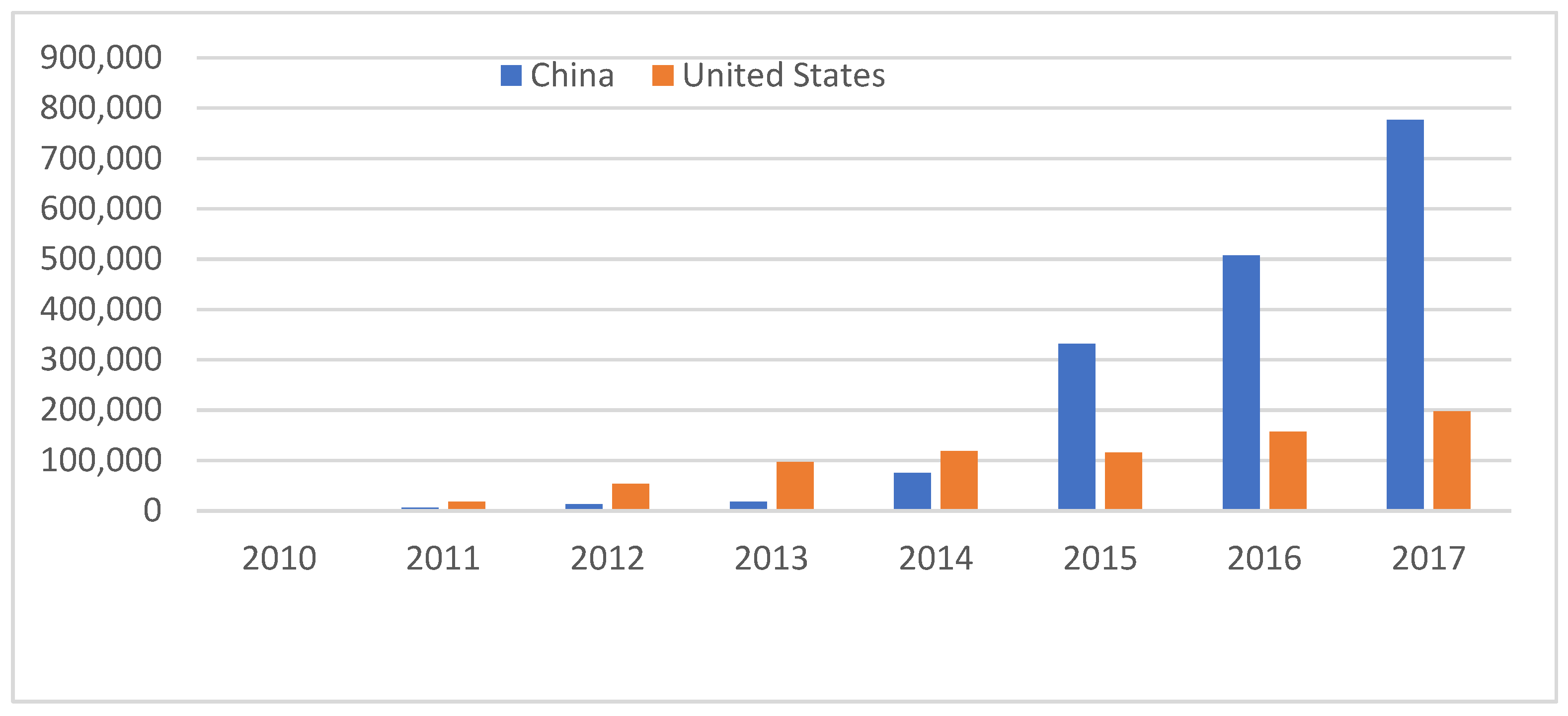In order to align the development of the automotive industry with the national sustainable development goals, the Chinese government explicitly designated the NEV industry, as represented by electric vehicles, as a strategic emerging industry in the 2010 Decision on Accelerating the Cultivation and Development of Strategic Industries. This decision provided a clear direction for the development of automotive industry policies. Subsequently, a series of specific supportive industrial policies, such as fiscal subsidies and tax exemptions, have been implemented to promote energy-saving vehicles and electric vehicles. These measures aim to encourage the adoption and use of environmentally friendly vehicles in China. The implementation of these policies has yielded significant results, as evidenced by the substantial growth in China’s sales of NEVs, surpassing the United States and becoming the global leader in NEV sales within a few short years (Figure 1). However, the data also indicate that continuous long-term efforts are required. As of 2017, although the sales of NEVs in China have shown rapid growth, the market penetration rate remains below 3% (Figure 2) [3].

The adoption of fiscal subsidies and tax exemptions as encouraging policies would significantly increase the financial burden on the country, making it difficult to sustain them in the long term. Furthermore, these policies may also tempt certain enterprises to engage in opportunistic behavior, seeking subsidies merely for short-term gains, thereby hindering their ability to focus on core technological research and achieve breakthroughs. The Chinese government urgently needs to seek more sustainable policies for the automotive industry to replace the existing fiscal subsidy policy.

Drawing inspiration from the European Union Emissions Trading Scheme (EUETS) policy and California’s Zero Emission Vehicle Mandate (ZEVM) initiative, China began planning in 2014 and officially launched the “Parallel Management of Corporate Average Fuel Consumption and New Energy Vehicle Credits for Passenger Car Enterprises” (hereinafter referred to as the dual-credit policy) in September 2017. As a significant alternative to financial subsidies in the Chinese automotive industry, the dual-credit policy differs from traditional industry incentives such as subsidies by shifting the focus from consumption to production [4]. The policy assesses both the corporate average fuel consumption credits (CAFC) and new energy vehicle (NEV) credits of vehicle manufacturers annually, requiring companies to achieve a total credit score of 0 or positive; otherwise, penalties will be imposed. Vehicle manufacturers with negative credit scores must compensate for their deficit by purchasing credits from manufacturers with positive credit scores through the credit trading market. The policy mechanism can achieve the transfer of policy cost internalization within the industry, effectively solve the financial burden problem brought about by fiscal subsidy policies, and make policy implementation more sustainable.

This policy not only effectively addresses the two major objectives of energy conservation and emissions reduction in the automotive industry and the promotion of NEV development through the assessment of two credits for manufacturers but also imposes higher R&D requirements on automotive companies through adjustments to the specific implementation details. For example, the policy sets higher requirements for fuel-efficient and emission-reducing technology innovation for fuel vehicles by adjusting the calculation of the CAFC credits based on the standard values for average fuel consumption. In the calculation of the NEV credits, the policy incorporates the range indicators of power batteries into the credit calculation criteria, imposing higher standards on the core power battery technology of NEVs, thereby providing more impetus and pressure for innovation in NEV technology R&D [5].

Recognizing the R&D pressure brought about by the dual-credit policy, vehicle manufacturers aspire to achieve breakthroughs in technological innovation. However, due to the cost pressure of R&D, vehicle manufacturers always seek to maximize their own interests in the game with stakeholders while striving to optimize investment in R&D. In the literature on the game between vehicle manufacturers and stakeholders, scholars divide the game into horizontal games between manufacturers [6] and vertical games between upstream (e.g., supplier) and downstream (e.g., distributor) players [7,8]. Although the current dual-credit policy mainly assesses the central player in the automotive industry chain—the vehicle manufacturer—it can have a radiating impact on upstream and downstream players through transmission from upstream and downstream enterprises, thereby contributing to collaborative and balanced development of the automotive supply chain [9]. Therefore, this paper focuses on analyzing the influence of the dual-credit policy in the game between upstream and downstream players. Since key breakthroughs in technological innovation may be achieved through vertical cooperation during the production and R&D stage rather than horizontal cooperation [10], this paper further focuses on the game between vehicle manufacturers and suppliers concerning R&D innovation.

This study aims to analyze the optimal R&D investment of component suppliers and vehicle manufacturers in the automotive industry chain under the dual-credit policy. This analysis requires comprehensive consideration of the actual circumstances of both parties within the Chinese automotive industry chain. The formation of the R&D alliance and the presence of a dominant entity within the industry chain will both result in deviations from the equilibrium point of optimal R&D investment for both parties. Specifically, the existence of the R&D alliance may lead to differences in profit maximization pursuits among major entities. The presence of a dominant entity will affect the sequence of the Stackelberg game [11]. Despite the emphasis on “strengthening the integration of vehicle and parts manufacturing” in China’s 2016 “Thirteenth Five-Year Plan for the Development of the Automotive Industry”, significant disparities persist in the design, research, and production capacities of Chinese automotive component suppliers. Data from the “2022 Automotive Supply Chain Development Report” indicate a continued weak collaborative research and development scenario between vehicle manufacturers and component suppliers. The global top 10 automotive component suppliers have shown minimal changes compared to previous years. For 12 consecutive years, Germany’s Robert Bosch has maintained its leading position. Conversely, China’s domestically produced core component competitiveness remains insufficient. Core engine technologies are still predominantly controlled by foreign suppliers, while core components heavily rely on imports. This underscores the substantial influence wielded by automotive component suppliers within the industry chain, positioning them in a dominant role.

Based on this, this paper constructs a Stackelberg dynamic game model to analyze the R&D strategic behaviors and stable equilibrium under the dual-credit policy between auto parts suppliers and vehicle manufacturers. Combined with the actual situation of the automotive industry chain in China, it reveals the evolutionary patterns of R&D levels and the mechanism for achieving stable R&D level equilibrium under the power structure dominated by uncooperative R&D between manufacturers and suppliers, with the suppliers in the lead, assuming bounded rationality. Furthermore, it explores strategies under the dual-credit policy to promote the equilibrium stability of R&D levels for both auto parts suppliers and vehicle manufacturers, aiming to better foster the sustained development of R&D in the automotive industry.

The primary contributions of this paper are as follows. First, it differs in its focus compared to the previous literature, which primarily concentrates on horizontal competition among vehicle manufacturers or vertical competition between vehicle manufacturers and dealers. This study centers on the strategic interactions between vehicle manufacturers, which are pivotal in R&D, and parts suppliers. Second, the differing assumptions about relevant decision-makers set this work apart. The prior literature often assumes decision-makers to be fully rational and capable of instantly achieving Nash equilibrium. In actual strategic interactions, decision-makers must continuously adapt their strategies to achieve optimality, a dynamic adjustment process that often requires a considerable amount of time. Consequently, investigating this dynamic adjustment process is crucial. Third, the influence of the power structure is introduced into the game model. Due to the asymmetric dependence between buyers and sellers within the supply chain, varying power structures exist [12,13]. Members holding dominant positions in terms of power possess the capability to control or influence the decisions of another member. The pricing and decisions of supply chain members may be influenced by the power structure [14]. Different power structures within the industry chain can affect the sequence of the Stackelberg game.

The rest of the structure is as follows. Section 2 reviews the relevant literature in recent years. Section 3 builds a two-stage Stackelberg game theoretical model and dynamic complex model. Section 4 conducts numerical simulation analysis, and Section 5 summarizes the main contributions of this paper.

2. Literature Review

To investigate the dynamic game dynamics of optimal R&D levels between vehicle manufacturers and parts suppliers under the dual-credit policy, we develop a two-stage static model and a dynamic game model based on the Stackelberg framework. Our research is situated within three primary literature streams: firstly, the examination of dual-credit policies; secondly, collaborative R&D focusing on innovation and sustainability goals; and thirdly, the analysis of complexity in dynamic game models within the supply chain.

2.1. The Dual-Credit Policy

Since the implementation of the dual-credit policy in China, scholars’ research on the policy has mainly focused on two aspects. Firstly, they have studied the impact of the policy on various aspects of the automotive industry. Boli (2023) and Haonanhe (2023) believe that the dual-credit policy can significantly promote green innovation and green technological innovation efficiency in automobile enterprises [1,15]. Rao (2022) believes that the policy has different effects on the financial performance of upstream and downstream automobile enterprises [9]. Yang (2022) believes that due to the pressure on R&D investment, the policy may not necessarily have a positive impact on the performance of automobile enterprises [16]. Xuli (2021) believes that there are differences in the significance and stability of R&D investment during the policy formulation period and implementation period [17]. Yitongwang (2023) finds that the strict CAFC scoring method in the dual-credit policy is more conducive to promoting the diffusion of electric vehicles than the strict NEV scoring method [18]. Lian (2023) believes that although the policy can curb the scale of fuel vehicles, it may not be able to promote fuel economy improvement, the development of new energy vehicle industry, and research and development cooperation [19]. Secondly, scholars have paid attention to coping strategies for policy implementation. Haonan He (2022) uses dynamic programming to study the optimal timing for automakers to invest in electrification under this policy [20]; Li Liu (2023) explores how manufacturers plan traditional vehicle product lines, new energy vehicle product lines, and hybrid product lines under this policy [21]; JiziLi (2022) studies the best strategies for automakers to obtain points [22]; Hui Yu (2023) uses multi-agent simulation to simulate the optimal innovation strategies of traditional automakers and new energy automakers under this policy [4], etc. This paper focuses on the first aspect of the policy’s dynamic impact on the R&D level of the automotive industry chain.

2.2. Innovative Collaborative R&D with Sustainability as the Goal

Due to institutional pressures, emerging developing country enterprises are not only concerned with profitability goals but also with sustainability goals [23]. Exploring sustainable innovation’s impact on product sustainability, resource efficiency, environmental pollution, and social responsibility is crucial [24].

The classic collaborative R&D for sustainable innovation can be divided into two categories. Firstly, horizontal collaborative R&D among enterprises. Duysters (2011) argues that the relationship between the complexity of alliance members and the innovation capability of the alliance presents an inverted U shape [25]. Hou Guangming et al. (2006) study the horizontal R&D collaborative innovation of duopolistic firms under a bilateral monopoly competition environment, assuming that there are exogenous and endogenous mixed spillover effects in R&D innovation [26]. Secondly, vertical collaborative R&D among enterprises. Cassiman and Veugelers (1998) study the manufacturing industry in Belgium and find that most cooperation agreements are vertical or involve collaboration with research institutions rather than horizontal. They discover that vertical collaboration is driven by external and complementary knowledge rather than sharing high costs or risks [27]. Liu Wei and Zhang Zijian (2009) establish a two-level vertical collaborative R&D model composed of manufacturers and suppliers to study issues such as bilateral moral hazard and collaborative R&D investment, and they discuss the optimal contract design for manufacturers to invest in R&D cooperation and the conditions for optimal cost-sharing under different R&D motivations of manufacturers and suppliers [28].

Open innovation describes the purposeful flow of knowledge across organizational boundaries, which is divided into inbound open innovation (the process of absorbing external knowledge through collaboration with business networks and other external entities) and outbound open innovation (the transfer of internal knowledge or technology to other technological fields, enterprises, or industries) [29]. Many scholars have noticed the impact of open innovation on sustainable innovation, considering open innovation a key aspect of a sustainable innovation strategy [30] or believing that open innovation has a mediating effect on sustainable innovation [31]. This complements traditional collaborative R&D for sustainable innovation with additional forms. This paper focuses on the automotive industry, which has certain technical barriers and tends to adopt classical collaborative R&D. The main focus of this paper is vertical collaborative R&D among enterprises.

2.3. Complexity Analysis of the Supply Chain Game

Complex dynamic theory is often used to study the stability of different systems, such as mechanics, weather, economics, and supply chain systems. It explores the results of external and internal disturbances that may cause changes in system equilibrium. Decision-making may undergo multiple adjustments, gradually approaching equilibrium and eventually reaching a stable state [32]. In this paper, we focus on its application in supply chain systems. The existing literature shows that conducting complexity analysis in supply chain systems has good research value and can be applied in multiple industries. Junhai Ma et al. (2022) conduct a complexity analysis of supply chain games in the low-carbon clothing industry and telecommunications industry [33]. Lou W (2018) analyzes the recycling industry in China’s color TV market [34]. Game models are often used in conjunction with supply chain complexity analysis, such as combining the Stackelberg model with complex dynamic theory, as in the work of Junhai Ma et al. (2022) in their study of optimal pricing in the low-carbon clothing supply chain and automobile manufacturers’ pricing strategies and equilibrium prices for green innovation enterprises [35]. Moreover, combining the Cournot model with complex dynamic theory, such as Zheng et al. (2019) studying the impact of R&D subsidy policies on the stability of R&D investment in the new energy vehicle industry [36]. Long et al. study the equilibrium stability of the Cournot game when there is asymmetric information and one-way R&D spillovers [37]. This paper adopts the method of combining the Stackelberg model with complex dynamic theory.

3. Model Construction and Analysis

3.1. Basic Assumptions

He, Q. (2022) [38] explores a duopoly supply chain structure within the automotive industry, comprising a supplier and a manufacturer. The supplier provides semi-finished products, such as engines, to the manufacturer at wholesale prices. The manufacturer then produces finished vehicles for retail sale in the final market. Substitutes exist for both the semi-finished auto parts and the finished vehicles in their respective markets. When making purchasing decisions, consumers take into account the retail price of vehicles and their energy efficiency. The following assumptions are made based on this context:

• The R&D levels of saving fuel for the supplier (s) and the manufacturer (m) are $x_s$ and $x_m$, respectively. The level of saving fuel for the final product is $x=x_s+x_m$; the retail price of the final product is $p$; the sensitivity of consumers to the level of saving fuel for the final product is $d$ (referred to as fuel sensitivity); the potential demand size of the final product in the market is $A$; and the market demand function for vehicles is: $q=A-p+d(x_s+x_m)$.
• In order to improve their respective R&D levels of saving fuel, both the supplier and the manufacturer conduct R&D on new products. Assume that the R&D costs are related to their respective R&D levels of saving fuel $x_i(i=s,m$) as well as their technological transformation capabilities. For simplicity, without affecting the analysis results, set the R&D cost coefficient of the auto parts supplier as 1, set the comparative R&D cost-efficiency coefficient of the manufacturer as $\rho$ to display the comparison between the R&D costs of the manufacturer and the supplier, borrow from the law of diminishing returns in scale, then the supplier’s R&D cost is ${x_s}^2/2$, while the manufacturer’s R&D cost is $\rho x_m{}^2/2$. Here, assume that the wholesale price of the auto parts supplier’s products is $w$, and the unit costs of both the auto parts supplier and the vehicle manufacturer are 0.

3.2. Construction of a Complex Dynamic Model under the Dual-Credit Policy for R&D Levels

The dual-credit policy requires the vehicle manufacturer to calculate the average fuel consumption (CAFC) credits and the new energy vehicle (NEV) credits and then determine the credits they need to purchase (or transfer). Assume that the actual fuel consumption levels of different vehicle models are the same. The negative difference between the actual value and the required standard value is the level of fuel saving $x$ (i.e., a negative value means a higher level of fuel saving; a positive value means a lower level of fuel saving). Therefore, the manufacturer’s CAFC credit is calculated as: $xq$.

When calculating the NEV credit, assume that the discount rate for NEV models is simplified to 1, the actual production proportion of new energy vehicles by the manufacturer is ${\delta }_1$, and the required proportion of new energy vehicles by the policy is ${\delta }_2$. Let $\delta ={\delta }_1-{\delta }_2$ be the difference between the actual production proportion and the required production proportion, and then the manufacturer’s produced NEV credit is: $\delta q$. Assuming that the unit price of points is $p_e$, summing up the above two credits, the manufacturer’s revenue from selling points is: $p_e(x+\delta )q$.

According to the above assumptions, the profit function of the supplier is as follows:

$${\pi }_s=qw-\frac{1}{2}{x}_s{}^2$$

(1)

The profit function of the manufacturer is as follows:

$$\begin{gathered} {\pi }_m=(p-w)q-\frac{1}{2}\rho x_m{}^2+p_e(x+\delta )q \\ =[p-w+p_e(x_s+x_m+\delta )][A-p+d(x_s+x_m)]-\frac{1}{2}\rho x_m{}^2 \end{gathered}$$

(2)

The Chinese automotive industry faces a challenge in the lack of competitiveness of core components, resulting in foreign suppliers maintaining control over the core technology of key components. Presently, there is a notable absence of robust R&D cooperation between vehicle manufacturers and component companies within the automotive supply chain. This paper examines the non-cooperative mode of R&D between suppliers and manufacturers. In this model, manufacturers and suppliers independently decide on their R&D levels, aiming to maximize their respective profits based on their profit functions.

In delineating the power dynamics within the automotive supply chain, the relationship between suppliers and manufacturers assumes distinct structures, notably categorized as the supplier-dominant non-cooperative mode (referred to as SN), manufacturer-dominant non-cooperative mode (referred to as MN), and vertical non-cooperative mode (referred to as VN). This classification reflects the prevailing influence of the power structure between these entities.

The Chinese automotive industry, despite its remarkable growth, still heavily depends on imported key high-quality components, especially pertaining to critical technologies like engine cores, which remain under the control of foreign suppliers. Notable examples include companies such as Bosch from Germany and Denso from Japan, each achieving substantial revenues of USD 40 billion in 2022. The reliance on foreign suppliers is particularly evident in terms of crucial components, such as the high-efficiency motors (with 97% efficiency) essential for new energy vehicles, which are predominantly sourced from European, American, and Japanese suppliers. Additionally, the automotive sector’s dependence on imported core chips further underscores the global nature of the supply chain, with foreign entities playing a central role. This asymmetric dependency implies that suppliers wield significant influence over key components, shaping the dynamics of the industry. Given this context, this study zooms in on the supplier-dominant non-cooperative mode (SN mode), aiming to dissect and comprehend the nuances of this power structure within the Chinese automotive supply chain.

In the SN model, the Stackelberg game process unfolds in two distinct steps. Initially, both the supplier and the manufacturer engage in determining their respective fuel-saving research and development (R&D) levels with the aim of maximizing profits, as guided by their individual profit functions. This initial step lays the foundation for optimizing each party’s contribution to the overall profitability of the system.

Subsequently, in the second step, the supplier assumes the role of the leader. In this leadership position, the supplier makes critical decisions, specifically focusing on establishing the wholesale price of the components denoted as “w”. Simultaneously, the manufacturer, acting as the follower in this game dynamic, calculates and sets the retail price of the final product based on the wholesale price, denoted as “p”.

This two-step process creates a sequential and strategic decision-making framework, where the initial R&D efforts set the stage for subsequent pricing decisions. The supplier’s leadership in determining the component prices influences the manufacturer’s pricing strategy for the end product, thereby shaping the overall economic dynamics within the Stackelberg game model. This structured approach allows for a nuanced understanding of how strategic choices at each step contribute to the overall profitability and sustainability of the supplier–manufacturer relationship in the context of fuel-saving technology development. The specific process is as follows:

$$\left.\begin{array}{c}\underset{x_s}{\max {\pi }_s}\\ \underset{x_m}{\max {\pi }_m}\end{array}\right\}\to \underset{w}{\max {\pi }_s\to }\underset{p}{\max {\pi }_m}$$

Using the backward induction method for calculation:

(1)

Derive the optimal $p$ based on the maximization of the manufacturer’s profit.

Set $\frac{\partial {\pi }_m}{\partial p}=0$ the best response is:

$$p=\frac{A+w+d(x_s+x_m)-p_e(\delta +x_s+x_m)}{2}$$

(3)

(2)

Substituting $p$ into the profit formula of the supplier, obtain the optimal $w$ based on the maximization of their profit.

Set $\frac{\partial {\pi }_s}{\partial w}=0$ the best response is:

$$w=\frac{A+d(x_s+x_m)+p_e(\delta +x_s+x_m)}{2}$$

(4)

(3)

Substituting the $w$ and $p$ into the profit functions of both parties, the marginal profits of both parties can be obtained.

$$\frac{\partial {\pi }_s}{\partial x_s}=\frac{(d+p_e)[A+d(x_s+x_m)+p_e(x_s+x_m+\delta )]}{4}-x_s$$

(5)

$$\frac{\partial {\pi }_m}{\partial x_m}=\frac{(d+p_e)[A+d(x_s+x_m)+p_e(x_s+x_m+\delta )]}{8}-\delta x_m$$

(6)

(4)

Set $\frac{\partial {\pi }_m}{\partial x_m}=0$ Obtain the optimal $x_m$

$$x_m=\frac{{(d+p_e)}^2{x}_s+(d+p_e)(A+\delta p_e)}{8\rho -(d+p_e{)}^2}$$

(7)

As the follower in the supply chain, the manufacturer assumes a naïve approach to adjust its fuel-saving R&D level $x_m$, assuming that the fuel-saving R&D level $x_s$ of the supplier remains unchanged in the two periods and adjusting its own level based on the optimal response function of the component supplier. On the other hand, the supplier adopts a gradient dynamic (GD) mechanism to adjust its fuel-saving R&D level, relying on its own marginal profit to adjust the level. Specifically, at each time period t, if the marginal profit is positive (negative), the component supplier will increase (decrease) the fuel-saving R&D level for the $t+1$ period. The complex dynamic adjustment system of both parties is as follows:

$$\left\{\begin{array}{l}{x}_m(t+1)=\frac{{(d+p_e)}^2{x}_s(t)+(d+p_e)(A+\delta p_e)}{8\rho -(d+p_e{)}^2}\\ x_s(t+1)=x_s(t)+k_1{x}_s(t)\{\frac{(d+p_e)[A+d(x_s+x_m)+p_e(x_s+x_m+\delta )]}{4}-x_s\}\end{array}\right.$$

(8)

3.3. Stability Analysis of the Equilibrium Point of the R&D Level

Based on the analysis of complex dynamic adjustment systems (8), the equilibrium point needs to meet the following:

$$\left\{\begin{array}{l}{x}_m=\frac{{(d+p_e)}^2{x}_s+(d+p_e)(A+\delta p_e)}{8\rho -{(d+p_e)}^2}\\ k_1{x}_s\{\frac{(d+p_e)[A+d(x_s+x_m)+p_e(x_s+x_m+\delta )]}{4}-x_s\}=0\end{array}\right.$$

(9)

Obtain equilibrium solutions as follow: $E_1(x^o{}_m,0)$, $E_2(x^{*}{}_m,x^{*}{}_s)$ where

$$x^o{}_m=\frac{(d+p_e)(A+\delta p_e)}{8\rho -(d+p_e{)}^2}$$

(10)

$$x^{*}{}_m=\frac{(d+p_e)(A+\delta p_e)}{8\rho -(1+2\rho )(d+p_e{)}^2}$$

(11)

$$x^{*}{}_s=\frac{2\rho (d+p_e)(A+\delta p_e)}{8\rho -(1+2\rho )(d+p_e{)}^2}$$

(12)

According to economic perspectives, a non-negative equilibrium point is meaningful and ${x^o}_m$ must be greater than 0. When at $E_1$, it indicates that the supplier does not invest in R&D at all, and all the R&D is carried out by the manufacturer. However, this is difficult to achieve in reality, as R&D investments exist simultaneously in both upstream and downstream. If $E_2$ is economic significance, it must also satisfy the condition, where ${x^{*}}_m>0, {{ x}^{*}}_s>0$, i.e.,

$$8\rho -(1+2\rho ){(d+p_e)}^2>0$$

(13)

To investigate the stability of the equilibrium points $E_1$ and $E_2$, the Jacobian matrix of system (8) is constructed as follows:

$$\begin{gathered} \left[\begin{array}{cc}\frac{\partial x_s(t+1)}{\partial x_s(t)}& \frac{\partial x_s(t+1)}{\partial x_m(t)}\\ \frac{\partial x_m(t+1)}{\partial x_s(t)}& \frac{\partial x_m(t+1)}{\partial x_m(t)}\end{array}\right] \\ =\left[\begin{array}{cc}1+k_1\{\frac{(d+p_e)[A+d(x_s+x_m)+p_e(x_s+x_m+\delta )]}{4}-x_s\}+k_1{x}_s(t)[\frac{{(d+p_e)}^2}{4}-1]& k_1{x}_s(t)\frac{{(d+p_e)}^2}{4}\\ \frac{{(d+p_e)}^2}{8\rho -{(d+p_e)}^2}& 0\end{array}\right] \end{gathered}$$

(14)

Substituting the coordinates of point $E_1$ into the Jacobian matrix yields:

$J(E_1)=\left[\begin{array}{cc}1+k_1\frac{(d+p_e)[A+(d+p_e)x_m+p_e\delta ]}{4}& 0\\ \frac{{(d+p_e)}^2}{8\rho -{(d+p_e)}^2}& 0\end{array}\right]$, The Jacobian matrix at the local stability of the equilibrium point must satisfy two characteristic roots: ${\phi }_i$, i = 1, 2, and $\left|{\phi }_i\right|<1$. The characteristic roots of $J(E_1)$, ${\phi }_1=0$, $\left.\left|{\phi }_1\right.\right|<1$; ${\phi }_2=1+k_1\frac{(d+p_e)[A+(d+p_e)x_m+p_e\delta ]}{4}$, $\left.\left|{\phi }_2\right.\right|>1$, $E_1(x^o{}_m,0)$ is an unstable equilibrium point.

Plugging in the specific value of point $E_2$ into the Jacobian matrix yields:

$$J(E_2)=\left[\begin{array}{cc}1+k_1{x}_s{}^{*}[\frac{{(d+p_e)}^2}{4}-1]& k_1{x}_s{}^{*}\frac{{(d+p_e)}^2}{4}\\ \frac{{(d+p_e)}^2}{8\rho -{(d+p_e)}^2}& 0\end{array}\right]$$

(15)

We set $\frac{\partial {\pi }_s}{\partial x_s}=0$ i.e.,

$$\frac{(d+p_e)[A+d(x_s+x_m)+p_e(x_s+x_m+\delta )]}{4}-x_s$$

The trace of the matrix:

$$T=1+k_1{x}_s{}^{*}[\frac{{(d+p_e)}^2}{4}-1]$$

(16)

The determinant of the matrix:

$$V=-\frac{k_1{x}_s{(d+p_e)}^4}{4[8\rho -{(d+p_e)}^2]}$$

(17)

The characteristic equation corresponding to the matrix is:

$$P(\phi )={\phi }^2-T\phi +V$$

(18)

In order for $E_2$ to be locally stable, in addition to satisfying condition (13), the discriminant of the characteristic equation must also satisfy:

$\Delta =T^2-4V>0$, and satisfy the Jury condition: $\left\{\begin{array}{l}1+T+V>0\\ 1-T+V>0\\ 1-V>0\end{array}\right.$, where

$$1-T+V=k_1{x}_s\frac{8\rho -(1+2\rho ){(d+p_e)}^2}{8\rho -{(d+p_e)}^2}>0 \mathrm{i}.\mathrm{e}., 8\rho -(1+2\rho ){(d+p_e)}^2>0$$

(19)

$$1+T+V=2+k_1\frac{2\rho (d+p_e)(A+p_e\delta )}{8\rho -(1+2\rho ){(d+p_e)}^2}\{\frac{{(d+p_e)}^2[4\rho -{(d+p_e)}^2]}{2[8\rho -{(d+p_e)}^2]}-1\}>0$$

i.e.,

$$k_1\frac{2\rho (d+p_e)(A+p_e\delta )}{8\rho -(1+2\rho ){(d+p_e)}^2}\{\frac{{(d+p_e)}^2[4\rho -{(d+p_e)}^2]}{2[8\rho -{(d+p_e)}^2]}-1\}>-2$$

(20)

3.4. Analysis of the Impact of Variables on the Stability of the R&D Level Equilibrium Point

3.4.1. Analysis of the Impact of the R&D Level Adjustment Speed $k_1$ on the Stability of the R&D Level Equilibrium Point

When analyzing the impact of the R&D adjustment speed on the dynamic evolution of the R&D level in the system, we refer to Dai [11] and define $m=(d+p_e)$ as the comprehensive reflection of the fuel consumption market. It represents the combined influence of the public’s fuel-saving and environmental awareness on the consumer market and the credit price in the credit trading market under the dual-credit policy. If $m$ is large, it indicates a high credit trading price or strong public awareness of fuel-saving and environmental protection, or both. If $m$ is small, it indicates that the public does not prioritize the fuel efficiency of vehicles or that the credit trading price is low. The magnitude plays an important incentive role in fuel-saving research and development in the automotive supply chain. The critical value can be obtained from Equation (20).

$$k_1{}^{*}=\frac{-2}{x^{*}{}_s[\frac{m^2(4\rho -m^2)}{2(8\rho -m^2)}-1]}$$

(21)

Because $x^{*}{}_s>0$ when $4\rho m^2-m^4>16\rho -2m^2$, $k_1<0$ be excluded.

When

$$4\rho m^2-m^4<16\rho -2m^2, k_1>0$$

$$k_1<-\frac{(8\rho -m^2-2\rho m^2)(16\rho -2m^2)}{\rho m(A+p_e\delta )(4\rho m^2-m^4-16\rho +2m^2)}$$

(22)

The upper limit of $k_1$, denoted as ${k_1}^{*}$, is the critical value. Therefore, when$0\le k_1<{k_1}^{*}$, the $E_2$ is locally stable.

Proposition 1. 

When the manufacturer chooses a naïve expectation and the supplier uses a gradient dynamical expectation, the Nash equilibrium point $E_2({x^{*}}_m,{x^{*}}_s)$is locally asymptotically stable if

$$0\le k_1<k_1{}^{*}=-\frac{(8\rho -m^2-2\rho m^2)(16\rho -2m^2)}{\rho m(A+p_e\delta )(4\rho m^2-m^4-16\rho +2m^2)}$$

3.4.2. Analysis of the Impact of the Difference in the Proportion of NEVs $\delta$ on the Stability of the R&D Level Equilibrium Point

When

$$4\rho m^2-m^4<16\rho -2m^2$$

$$1+T+V=2+k\frac{2\rho (d+p_e)(A+p_e\delta )}{8\rho -(1+2\rho ){(d+p_e)}^2}\{\frac{{(d+p_e)}^2[4\rho -{(d+p_e)}^2]}{2[8\rho -{(d+p_e)}^2]}-1\}>0$$

(23)

i.e.,

$$2+k_1\frac{2\rho m(A+p_e\delta )}{8\rho -(1+2\rho )m^2}\frac{4\rho m^2-m^4-16\rho +2m^2}{2(8\rho -m^2)}>0$$

(24)

After derivation, the following is obtained:

$$\delta <\frac{-2(8\rho -m^2)[8\rho -(1+2\rho )m^2]}{p_e{k}_1\rho m(4\rho m^2-m^4-16\rho +2m^2)}-\frac{A}{p_e}$$

(25)

The upper limit of $\delta$, denoted as ${\delta }^{*}$, is the critical value. Therefore, when $0\le \delta <{\delta }^{*}$, the $E_2$ is locally stable.

Proposition 2. 

Consider two firms with heterogenous strategies where the manufacturer chooses a naïve expectation and the supplier uses a gradient dynamical expectation, the Nash equilibrium point $E_2(x^{*}{}_m,x^{*}{}_s)$is locally asymptotically stable if

$$0<\delta <{\delta }^{*}=\frac{-2(8\rho -m^2)[8\rho -(1+2\rho )m^2]}{p_e{k}_1\rho m(4\rho m^2-m^4-16\rho +2m^2)}-\frac{A}{p_e}$$

3.4.3. Analysis of the Impact of the R&D Cost-Efficiency $\rho$ on the Stability of the R&D Level Equilibrium Point

When

$$4\rho m^2-m^4<16\rho -2m^2$$

Transforming Equation (23) into the following form:

$$2k_1\rho m(A+p_e\delta )(4\rho m^2-m^4-16\rho +2m^2)+4[8\rho -(1+2\rho )m^2](8\rho -m^2)>0$$

(26)

We find that this equation is a quadratic equation with respect to $\rho$. Therefore, we can determine two critical values, ${{\rho }^{*}}_1$ and ${{\rho }^{*}}_2$.

$${\rho }^{*}{}_1=-\frac{32m^2-4m^4+M-2\delta k_1{m}^3{p}_e-2A{k}_1{m}^3+\delta k_1{m}^5{p}_e+A{k}_1{m}^5}{8(8m^2+4A{k}_{1}m-a{k}_1{m}^3+4\delta k_{1}m{p}_e-\delta k_1{m}^3{p}_e-32)}$$

(27)

$${\rho }^{*}{}_2=\frac{4m^4-32m^2+M+2\delta k_1{m}^3{p}_e+2A{k}_1{m}^3-\delta k_1{m}^5{p}_e-A{k}_1{m}^5}{8(8m^2+4A{k}_{1}m-a{k}_1{m}^3+4\delta k_{1}m{p}_e-\delta k_1{m}^3{p}_e-32)}$$

(28)

where

$$M=\sqrt{m^5(A^2{k}_1{}^2{m}^5+4A^2{k}_1{}^2{m}^3+4A^2{k}_1{}^{2}m+2A\delta k_1{}^2{m}^5{p}_e+8A\delta k_1{}^2{m}^3{p}_e+8A\delta k_1{}^{2}m{p}_e)-8A{k}_1}$$

The range of values for $\rho$ depends on the coefficient of ${\rho }^2$. When $8(m^2-4)[k_{1}m(A+p_e\delta )-8]>0$, the equation opens upward, and the values of $\rho$ are $0<\rho <{{\rho }^{*}}_1$ and $\rho >{{\rho }^{*}}_2$. When $8(m^2-4)\left[k_{1}m\right(A+p_e\delta )-8]<0$, the equation opens downward, and the values of $\rho$ are ${{\rho }^{*}}_1<\rho <{{\rho }^{*}}_2$.

Proposition 3. 

When the manufacturer chooses a naïve expectation and the supplier uses a GD expectation, the Nash equilibrium point $E_2({x^{*}}_m,{x^{*}}_s)$is locally asymptotically stable if $8(m^2-4)\left[k_{1}m\right(A+p_e\delta )-8]>0$, then $0<\rho <{{\rho }^{*}}_1$ and $\rho >{{\rho }^{*}}_2$, or if $8(m^2-4)\left[k_{1}m\right(A+p_e\delta )-8]<0$, then ${{\rho }^{*}}_1<\rho <{{\rho }^{*}}_2$ where

$${\rho }^{*}{}_1=-\frac{32m^2-4m^4+M-2\delta k_1{m}^3{p}_e-2A{k}_1{m}^3+\delta k_1{m}^5{p}_e+A{k}_1{m}^5}{8(8m^2+4A{k}_{1}m-a{k}_1{m}^3+4\delta k_{1}m{p}_e-\delta k_1{m}^3{p}_e-32)}$$

$${\rho }^{*}{}_2=\frac{4m^4-32m^2+M+2\delta k_1{m}^3{p}_e+2A{k}_1{m}^3-\delta k_1{m}^5{p}_e-A{k}_1{m}^5}{8(8m^2+4A{k}_{1}m-a{k}_1{m}^3+4\delta k_{1}m{p}_e-\delta k_1{m}^3{p}_e-32)}$$

4. Numerical Simulation and Analysis

Because discrete dynamic systems under normal circumstances do not have analytic solutions, this section will apply numerical simulation methods to analyze the evolutionary characteristics of the price evolution dynamic system (8). We focus on the simulation and verification of the theoretical analysis in the previous sections. It explores the dynamic impact of various factors on the stability of discrete systems (8) and provides corresponding management interpretations. We will use 1D and 2D bifurcation diagrams, maximum Lyapunov exponents, singular attractors, initial-value sensitivity, and the basin of attraction, among other tools, to display the stability, bifurcation, chaos, and other states of the system.

The bifurcation diagram of system (8) with respect to $k_1$ is shown in Figure 3, where $A=10$, $d=0.2$, $p_e=1$. From the figure, it can be observed that when $k_1<0.4062$, there exists a Nash equilibrium ($x_s{}^{*}$, $x_m{}^{*}$) = (3.4239, 6.8478). As $k_1$ gradually increases, system (8) experiences a flip bifurcation at $k_1{}^{*}=0.4062$ and then goes through 8-period doubly periodic and 16-period triply periodic bifurcations before finally falling into chaos at $k_1=0.5268$. The maximum Lyapunov exponent (MLE) in Figure 3 is also calculated, with MLE = 0 indicating that the system is experiencing a flip bifurcation and MLE > 0 indicating that the system is in a chaotic state. The evolutionary trajectory of the system in Figure 3 indicates that if the R&D level adjustment of the supplier is too large, it may cause fluctuations in both the supplier’s and manufacturer’s R&D levels and even lead to chaos. Thus, small R&D level adjustments are conducive to stable R&D.

The evolutionary trajectory of the system with respect to $\delta$ is shown in Figure 4. Other parameters are set: $A=10$, $d=0.2$, $p_e=1.2$, $\rho =0.96$, $k_1=0.21$, and when $\delta <{\delta }^{*}=0.1894$, system (8) is in a stable state; when $\delta >{\delta }^{*}$, the system exhibits a bifurcation. From Figure 4, it can be observed that as the system is in a stable state, the R&D level increases with the increase $\delta$, which means that when the dual-credit policy requires a higher proportion of NEVs than the actual proportion of enterprises, suppliers and manufacturers are willing to invest more in R&D.

Compared to the 1D bifurcation diagram, the 2D bifurcation diagram is more advantageous in simulating the complexity of nonlinear systems. Figure 5 depicts the two-dimensional bifurcation diagram for the ($k_1$,$\delta$), with other parameters held $A=10$, $d=0.2, p_e=1,$ $\rho =1$. Different colors are used to label different cycle-splitting regions in the figure, where brown indicates that the system is in a stable state, and green, orange, yellow, dark green, red, blue, and purple represent the system being in 2–8 period bifurcations respectively. Black signifies that the system is in a chaotic state. From Figure 5, it can be observed that regardless of the value of $\delta$, the system is always in a stable state when $k_1$ is small. However, when $k_1$ is large, the value of $\delta$ does not affect whether the system is in a chaotic state or not. Therefore, the speed of the R&D level adjustment by suppliers has an important impact on the stability of R&D in reality.

Figure 6 depicts the influence of $\rho$ on the stability of system (8) with other parameters held $A=10$, $d=0.1{, p}_e=1.15{, k}_1=0.39, \delta =0.5$. When $8(m^2-4)\left[k_{1}m\right(A+p_e\delta )-8]>0$, $0<\rho <{{\rho }^{*}}_1=0.15$ and $\rho >{{\rho }^{*}}_2=1.1736$, system (8) is in a stable state. However, due to the negative R&D levels when $\rho <{{\rho }^{*}}_1$, a bifurcation diagram is not provided in Figure 6. The system exits chaos at $\rho <1.1736$, and the R&D levels remain unstable. When $\rho >1.1736$, there exists a Nash equilibrium for the R&D level. This indicates that when the market is insensitive to fuel economy levels $(d+p_e)$ or the potential demand $A$ is limited, it is more favorable for the R&D level to be stable if manufacturers have higher comparative efficiency in terms of R&D costs compared to suppliers.

Figure 7 and Figure 8 show the bifurcation diagrams of the system with respect to $d$ and $p_e$. Figure 7 depict the bifurcation diagrams of the system with respect to $d$ for different values of $p_e$, while the other parameters are $A=10$, $p_e=1.15$, $k_1=0.42$, $\rho =1.2$, $\delta =0.71$. It is observed that as $p_e$ increases, the stable range of $d$ decreases, and vice versa. This suggests that when the unit price of credit sales is high, consumers who are highly fuel-economy-sensitive may be less inclined to engage in R&D, which could negatively impact the stability of R&D efforts. On the other hand, Figure 8 display the bifurcation diagrams of the system with respect to $p_e$ for different values of $d$, while the other parameters are $A=10$, $p_e=1.15$, $k_1=0.4$, $\rho =1$, $\delta =0.6$. It can be concluded that as $p_e$ increases, the stability of system (8) is more compromised. However, when consumers are not very sensitive to fuel consumption, a moderate increase in the unit price of credit sales does not significantly affect the stability of the system.

Figure 9 depicts the attractors of the system for different values of $d$, while the other parameters are $A=10$, $p_e=1.1$, $k_1=0.42$, $\rho =1.2$, $\delta =0.71$. The analysis of Figure 9 reveals a noteworthy trend: as the sensitivity to fuel economy increases, the evolution of the system becomes more intricate. The progression unfolds in a deterministic yet seemingly random manner, suggesting a heightened level of complexity in the dynamics at play. The system’s movement toward a chaotic state is particularly evident. In this chaotic state, the system exhibits a high degree of sophistication, indicating that the economic dynamics become challenging to predict with precision. The unpredictability introduced during this chaotic evolution implies that forecasting economic outcomes under heightened fuel economy sensitivity becomes a more intricate task. The intricate interplay of various factors and the emergence of seemingly random patterns underscore the need for adaptive and resilient forecasting models that can account for the nuanced complexities inherent in economic systems during such states of heightened sensitivity. This observation emphasizes the importance of considering dynamic and evolving factors when making economic forecasts, particularly in contexts where the sensitivity to fuel economy plays a crucial role in shaping system behavior.

The sensitivity of the initial values is an important characteristic of chaos, which is exemplified in Figure 10a,b. The slight difference in the initial values (0.0001) leads to significant differences in the evolution of the R&D levels over time. Other parameters are set as follows: $A=10$, $p_e=1$, $k_1=0.42$, $\rho =1.2$, $\delta =0.71$, $d=0.28$. “$t$” represents the number of iterations (i.e., the number of times the supplier and manufacturer play their game). For example, Figure 10a shows that when the initial R&D levels ($x_s$, $x_m$) are (6.1, 2.6) and (6.10001, 2.6), respectively (at this time, the difference in the initial R&D level of the supplier is small), with the increase in the number of iterations $t$, a large difference will appear in the research and development level $x_s$ under the chaotic state.

In Figure 11, Figure 12, Figure 13 and Figure 14, we introduce the attraction domain to study the influence of parameters $k_1$, $d$, $\delta$, $\rho$ on the evolutionary trajectory of system (8). The attraction domain refers to a set of initial R&D levels converging to the same attractor after a series of games. In the economic society, when all the points in the attraction region (yellow region) converge to an equilibrium point, then the equilibrium point is the Nash equilibrium point, and any R&D level in the attraction domain will converge to Nash equilibrium after many games. If the initial development level is in the escape zone (blue region), the system eventually falls into divergence. In Figure 11a, when the initial R&D level of the enterprises is in the attraction domain, the R&D level will become stable after iteration, and the attractor (red dot) at this time is the Nash equilibrium. As the adjustment speed $k_1$ increases, the attractor domain gradually narrows. In Figure 11b,c, the system is in a 2-period and 8-period state, respectively. When $k_1$ = 0.6, the system is in a chaotic state, which means that if the initial R&D level is in the attraction domain of Figure 11d, the system will converge to a chaotic attractor. Figure 12, Figure 13 and Figure 14 show the influence of the fuel economy sensitivity $d$, new energy vehicle share $\delta$ and R&D cost efficiency $\rho$ on the attraction domain, but different from Figure 11, the R&D level in the equilibrium state of Figure 12, Figure 13 and Figure 14 is closely related to parameters $d$, $\delta$, $\rho$, but not to $k_1$, which can be seen from Formulas (10)–(12). Therefore, the influence of each parameter on the size of the attractive domain is different. In Figure 12 and Figure 13, the attraction domain increases with the increase in d and sigma, while Figure 14 shows that the attraction domain decreases as $\rho$ increases; when $\rho$ = 1.1736, the system finally converges to Nash equilibrium.

5. Conclusions and Discussion

This study delves into the influence of a dual-credit policy on the research and development (R&D) levels within automotive supply chains, encompassing both suppliers and manufacturers. It scrutinizes the dynamic game behavior and equilibrium stability of R&D levels, particularly in an uncooperative R&D environment characterized by a dominant supplier power structure. The paper aims to identify strategies that can foster equilibrium and stable R&D levels in these supply chains. Additionally, it explores the impact of variables such as the R&D level adjustment speed, the proportion of new energy vehicles (NEVs), and R&D cost-efficiency on the equilibrium stable point.

The ultimate goal is to provide theoretical insights and inspiration for government bodies and automotive companies in formulating policies to sustain R&D levels. The key research conclusions are outlined below:

(1)

When the government sets the standard for the proportion of NEVs in the dual-credit policy, there is an appropriate gap between the standard and the actual proportion of manufacturers. This can promote suppliers and manufacturers to increase R&D investment and improve R&D levels. However, if the gap exceeds a certain threshold, it will lead to the bifurcation and chaos of the R&D level game system.

(2)

When the dominant supplier in the supply chain adopts the GD R&D level adjustment mechanism, if the adjustment speed exceeds the stable condition, the R&D level game system will exhibit chaos and bifurcation, making it difficult to stabilize the research and development level.

(3)

When consumers are not sensitive to fuel consumption or when the market demand is limited, the higher R&D efficiency of suppliers is more conducive to the stability of the research and development level system.

(4)

When consumers are highly sensitive to fuel consumption, higher credit trading prices are not suitable for stabilizing the R&D level.

(5)

Increasing consumer sensitivity to fuel consumption leads to increased complexity in the evolution of the research and development level system.

In the intricate game of R&D levels within the automotive supply chain, the nonlinear characteristics significantly heighten the sensitivity of R&D levels to the initial conditions. Key parameters, such as the pace at which the leader in the supply chain adjusts the R&D levels, consumer fuel consumption sensitivity, and the set proportion of new energy vehicles (NEVs) in the dual-credit policy, wield substantial influence over the trajectory of R&D evolution. Consequently, automotive companies must meticulously consider these parameters when strategizing R&D investments, acknowledging the challenge of controlling many of these influential factors.

Addressing these parameters through policy adjustments offers a compelling advantage in stabilizing R&D levels. The findings of this research carry considerable weight in offering reference points and strategic recommendations for government entities aiming to craft policies that foster stability in R&D levels:

(1)

For companies in a leadership position, a smaller adjustment speed of the R&D level is beneficial for achieving stability in the automotive supply chain R&D level. The government can limit the adjustment speed of the R&D level of companies.

(2)

The difference in the proportion of NEV sales in the dual-credit policy should be within a certain threshold to maintain system stability and improve the R&D level of the entire supply chain. The proportion standard in the dual-credit policy should be based on the actual proportion of NEVs by manufacturers, and the difference between the two should not be too large.

(3)

Improving the R&D efficiency of suppliers is more effective in stabilizing the R&D level. It is recommended that the government issue policies to improve the R&D efficiency of component suppliers in the automotive supply chain (such as encouraging R&D cooperation among suppliers).

(4)

When regulating the credit trading price, attention should be paid to consumer fuel consumption sensitivity in order to achieve stability in the R&D level system. When consumers have a high fuel consumption sensitivity, stricter proportion standards in the dual-credit policy (such as increasing the fuel consumption standards or the proportion of NEVs) can be formulated to reduce the credit supply in the credit trading market, thereby controlling the credit trading price and stabilizing the R&D level in the automotive supply chain.

This article presents opportunities for the refinement of several aspects:

(1)

Model Construction Complexity: During the model construction phase, the intricate nature of the analysis and computational complexities led to a focus on the interaction between suppliers and manufacturers exclusively. Looking ahead, the integration of the government into the model could offer a more comprehensive three-party dynamic analysis. This inclusion would provide a holistic understanding of the automotive supply chain dynamics by accounting for the government’s influence and policies.

(2)

Cooperation in the Automotive Industry: The utilization of a non-cooperative model in the analysis stems from the perceived inadequacy of the existing cooperation between suppliers and manufacturers, as evidenced by the 2022 automotive industry report data. As collaboration within the automotive industry’s supply chain evolves, a potential avenue for improvement lies in employing a cooperative model for analysis. This adjustment would better capture and analyze scenarios where enhanced cooperation becomes a defining characteristic of the industry.

(3)

Power Dynamics and Indigenous Technological Advancements: The power structure embedded in the model currently reflects a supplier-dominant scenario, a reflection of the heavy reliance on foreign imports for core components in China, particularly evident in the 2022 industry data. It is crucial to acknowledge that this structure is contingent on the prevailing circumstances. If indigenous technological advancements alter the landscape, leading to shifts in the positions of suppliers, the model settings must be adapted accordingly. This foresight ensures the model’s relevance in dynamically changing industrial landscapes.