Multi-Objective Design of UAS Air Route Network Based on a Hierarchical Location–Allocation Model

Abstract

This research concentrates on the Unmanned Aircraft System (UAS) demand sites’ hierarchical location–allocation problem in air route network design. With demand sites (locations where UAS operations are requested) organized and allocated according to the spatial hierarchy of UAS traffic flows, the hierarchical structure guarantees resource conservation and economies of scale through traffic consolidation. Therefore, in this paper, the UAS route network with a three-level hierarchy is developed under a multi-objective decision-making framework, where concerns about UAS transportation efficiency from the user side and construction efficiency from the supplier side are both simultaneously considered. Specifically, a bi-level Hybrid Simulated Annealing Genetic Algorithm (HSAGA) with global and local search combined is proposed to determine the optimal number, location, and allocation of hierarchical sites. Moreover, using the information of site closeness and UAS demand distribution, two problem-specific local search operators are designed to explore elite neighborhood regions instead of all the search space. A case study based on the simulated UAS travel demand data of the Beijing area in China was conducted to demonstrate the effectiveness of the proposed method, and the impact of critical parameter settings on the network layout was explored as well. Findings from this study will offer new insights for UAS traffic management in the future.

1. Introduction

Substantial growth in Unmanned Aircraft System (UAS) civilian applications is expected in both remote and congested urban areas, including infrastructure surveillance, agricultural support, air passenger and cargo transportation, etc. Given registration trends and market development, the Federal Aviation Administration (FAA) forecasts that the urban UAS service market in the U.S. will reach approximately USD 115 billion by 2035, equivalent to 30% of the present commercial air transportation market [1]. Specifically, the emerging concept of Urban Air Mobility (UAM) using a UAS for passenger transport and cargo delivery will shift travel to the third dimension and, thus, escape severe ground traffic congestion in large cities, having a potential annual market value in the billions [2]. Despite the enormous economic potential, there is currently no system in place to enable and safely manage the widespread use of UASs [3]. This leads to the novel UAS Traffic Management (UTM) concept, which refers to a system and a set of services that provide the necessary information and procedures to support safe and efficient UAS operations [4]. One critical UTM functionality is the design of airspace, which ensures that the airspace is configured for the most-efficient UAS operations in light of the traffic demand. Currently, the operating altitudes for civilian UASs are concentrated at or below 400 ft Above Ground Level (AGL) [5].

1.1. Related Work

Table 1 gives a summary of previous studies on the UAS-oriented airspace configuration. A clear consensus on the optimal type of airspace design that should be implemented has still not been reached [6]. Several studies argue that the airspace should be unrestricted and fully open to autonomous vehicles [7,8], while others state that predefined routes are required to handle high traffic densities [9,10]. Although an unstructured airspace grants great UAS flight flexibility, computational complexity will inherently increase with the trajectory scale. For instance, in case multiple trajectories occupy the same space at the same time, detailed 4D trajectories of other UAS operations in the area of travel should be obtained before launch [11]. This has both security and privacy issues since complete trajectory information can reveal the intent of the operations. In contrast, a structured airspace eliminates the need for detailed trajectory information by guiding origin–destination traffic to fly along explicit three-dimensional routes. In this way, traffic management complexity can be greatly reduced from 4D to 1D. Therefore, the route-based airspace functional design that guides UAS flights in it has received special attention in recent studies [11,12].

An air route can be defined as follows: the airspace is abstracted as a directed graph with a set of route segments connecting multiple demand sites. Direct UAS routing between the departure and destination has been widely studied in low-altitude airspace, where UAS flight is constrained by complicated environmental factors and obstacles. Path planning methods such as the geometry method, velocity space method [13], and graph search method [12,14] have been proposed to generate the most-cost-effective route while avoiding obstacles. However, these works mainly focused on route planning for one single aircraft. When applied to large-scale UTM scenarios, such individual-optimal planning models have the drawback of limited system observability. For instance, some major routes are popular pathways that UASs could have shared, but these resources are not fully utilized due to separate individual decisions. Hence, network-based UAS routing has recently been researched in the literature for its advantage in traffic demand consolidation and dissemination [15,16,17].

Unlike point-to-point direct routing, a public route network is constructed in network-based models by concentrating UAS flow on a certain number of routes to produce economies of scale and to allow infrastructure cost savings. Considering that UAS route network design can significantly affect the operational performance, a range of critical factors influencing UAS route choice decisions are investigated, including the network topology, routing strategy, and associated optimization algorithm [16,17,18]. In general, the route network should be designed to meet UAS traffic demand with minimal total operating costs, while actual conditions for application such as UAS performance limitation and airspace restriction should also be considered at the same time.

However, most of the above studies regard the route network as a single-level entity with one kind of route property. It is well known, instead, that, in existing transportation networks, resources are typically managed and controlled in a hierarchical manner [19,20,21]. That is, route links should be classified into hierarchies (or levels) according to the flow of the traffic that they carry. Such a network hierarchy is essential to reflect both the underlying organizational structure of UAS traffic demand (e.g., long-haul flights for inter-regional movement vs. short-haul flights within a Metropolitan area) and the functional division of the associated service provision (e.g., the main route, which supports high-volume flow, vs. the branch route, which accommodates local traffic). For instance, aviation markets commonly use the hub network structure for profit maximizing, and a recent review was given in [22], where hub–spoke airlines can serve a large number of destinations with a high frequency. Apart from the traditional one-hub-type and one-transportation-mode network, multi-layer hub networks involving different hub types across multiple transportation service layers (e.g., air, ground, and underground) are also widely studied [23,24,25]. Accordingly, two representative studies adopted the two-level hub–spoke hierarchical topology for urban on-demand UAS route network design [2,26], where the backbone network is formed at the upper level and the local access network is formed at the lower level. However, only two types of routes were considered in both works, while the hierarchy of routes should be classified into more-detailed levels to increase the functional completeness of the UAS route system and to maximize the adaptive ability between the airspace spatial layout and UAS demand distribution. Besides, previous works focused mainly on minimizing the UAS travel costs from the user side, while the launch site construction resource from the supply side was barely considered in the network design. Generally, a better transportation service will be offered to UASs in the presence of more direct connections. But, there exist upper bounds for the resources of UTM service providers to support and supervise such operations. In this case, two conflicting interests from different stakeholders, i.e., the user side and supply side, pose a design trade-off, which makes the problem even more complicated.

Table 1. Summary of previous studies for UAS-oriented airspace configuration.

Category	Characteristic	Article	Main Contribution
Airspace structure	Unstructured	[7,8]	Assessed low-altitude airspace capacity after the introduction of UAS operations.
	Structured	[9,10,11,12]	Proposed several UAS airspace structural designs (e.g., layers, lanes, or blocks) and investigated the influence of the airspace structure on performance (e.g., capacity, risk).
Path planning	Single vehicle	[12,13,14]	Generated safe and cost-effective paths for UASs independently by using algorithms such as A* and Rapidly-Exploring Random Tree.
	Multiple vehicles	[15,16,17]	Feasible routes designed between UAS Origin–Destination (OD) pairs within sectored or gridded airspace.
Route network type	Single-layer network	[16,17,18]	Single-level route network connecting conflict-free nodes and links that are away from hazardous airspace.
	Multi-layer network	One transport mode:  [2,19,20,21,26]	Extracted the hierarchical organization of the transportation network and identified UAS demand points as hubs or spokes.
		Multimodal transport: [23,24,25]	Interconnected layers via hub locations to integrate two or more different transportation modes.

Table 1. Summary of previous studies for UAS-oriented airspace configuration.

Category	Characteristic	Article	Main Contribution
Airspace structure	Unstructured	[7,8]	Assessed low-altitude airspace capacity after the introduction of UAS operations.
	Structured	[9,10,11,12]	Proposed several UAS airspace structural designs (e.g., layers, lanes, or blocks) and investigated the influence of the airspace structure on performance (e.g., capacity, risk).
Path planning	Single vehicle	[12,13,14]	Generated safe and cost-effective paths for UASs independently by using algorithms such as A* and Rapidly-Exploring Random Tree.
	Multiple vehicles	[15,16,17]	Feasible routes designed between UAS Origin–Destination (OD) pairs within sectored or gridded airspace.
Route network type	Single-layer network	[16,17,18]	Single-level route network connecting conflict-free nodes and links that are away from hazardous airspace.
	Multi-layer network	One transport mode:  [2,19,20,21,26]	Extracted the hierarchical organization of the transportation network and identified UAS demand points as hubs or spokes.
		Multimodal transport: [23,24,25]	Interconnected layers via hub locations to integrate two or more different transportation modes.

1.2. Motivation

Inheriting the concept of network hierarchy, a three-level UAS route network was designed in this paper, which is consistent with UAS demand patterns and corresponding flight service provisions. Such a hierarchy is also beneficial to the transportation-efficient objective from the user side and the construction-efficient objective from the supply side. That is, as the connection of the whole route network is kept by a certain number of routes, the total UAS transport cost can be decreased by the economies of scale of the consolidated flow, and the resource quantities needed for the overall network construction can be greatly reduced as well. In detail, the designed route network was assumed to consist of three types of locations, i.e., the primary site, secondary site, and ordinary site, in order of importance, and three types of route configurations, i.e., the main route connecting the primary site, the trunk route connecting the primary site and secondary site, and the branch route connecting the secondary site and ordinary site. To determine the appropriate hierarchy, the following questions must be answered. First, for each demand site, which hierarchy type it belongs to should be identified since the site hierarchy heavily affects all subsequent network modeling issues. Second, high-level sites such as primary and secondary sites are the backbones of the transportation network. How to decide about the optimal number of high-level sites should be investigated to balance the trade-off between UAS transportation efficiency and site construction resource quantity. Third, considering each site (except the primary sites) should be allocated to the next higher hierarchy, which secondary (ordinary) site should be allocated to which primary (secondary) site is a complex task. In general, this paper attempted to answer the above questions in the hierarchical route network design.

1.3. Summary of Contributions

Most existing airspace design methods for UAS operations assume a homogeneous route property, i.e., all routes have an equal level and importance. This paper overcomes this limitation by dividing routes into hierarchies based on the an uneven UAS spatial distribution, allowing for better coordination between airspace layout and traffic demands. Besides, instead of the one-sided pursuit of UAS transportation cost minimization, the proposed method provides a new insight into the trade-off between UAS transportation efficiency and airspace infrastructure construction, which assists sustainable decision-making in future UAS airspace configurations. Specifically, we believe that a well-structured UAS public route network will also contribute to the sustainable development of the airspace system in terms of efficient and flexible resource utilization. For instance, massive UAS operations can be accommodated collaboratively with enhanced predictability across predefined routes within the network. Meanwhile, the redundancy in individual UAS route planning will also be reduced, which is essential for the sustainable and scalable growth of the UAS industry.

The proposed method has the following three traits:

(1)

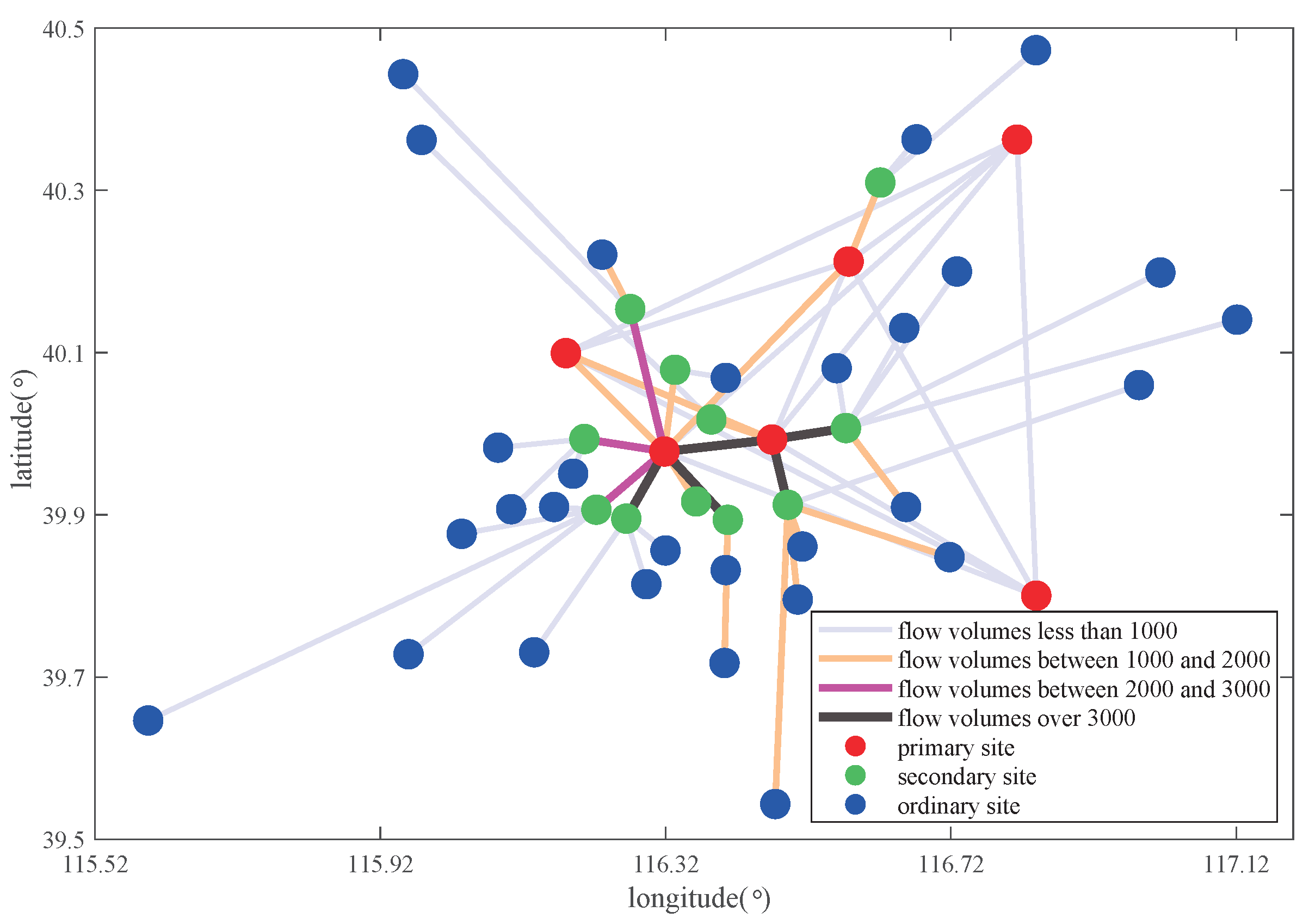
A typical three-level hierarchy is adopted to service UAS traffic demand at multiple scales, i.e., UAS demand sites are categorized into primary, secondary, and ordinary sites, and route functions between pairs of sites are classified as the main route, trunk route, and branch route correspondingly.

(2)

A multi-objective transportation–construction-efficient model is formulated to provide informed choices among a range of Pareto-optimal solutions, where operational constraints on the airspace hazard, the quantity restriction, and the UAS performance limit are also considered in the model.

(3)

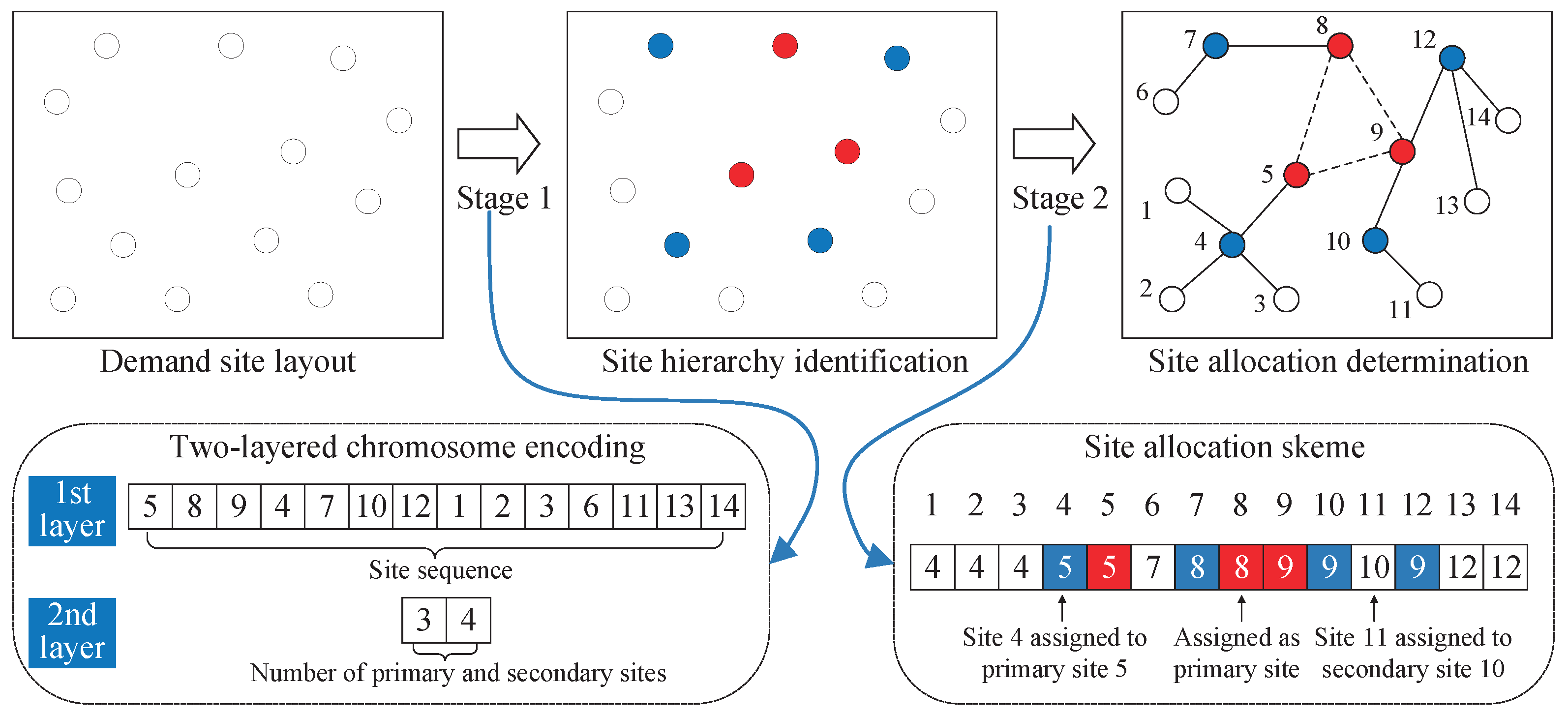
For the sake of computation, a bi-level hybrid Simulated Annealing Genetic Algorithm (HSAGA) is proposed for the balance between exploitation and exploration, where a genetic global search framework is hybridized with two problem-specific local search operators.

The remainder of this paper is organized as follows. The key assumptions of this study and the problem formulation are discussed in Section 2. The determination of the demand site hierarchy and the details of the proposed bi-level algorithm are presented in Section 3. A case analysis and a sensitivity analysis for the validation of the are performed in Section 4. Finally, Section 5 concludes the paper and highlights the future works to be conducted in line with this paper.

2. Mathematical Formulations

This section discusses the basic formulation of the multi-objective site location–allocation problem within a three-level UAS air route network.

2.1. General Assumption

The following assumptions were made for the hierarchical UAS route network design in this study. Figure 1 sketches a three-level hierarchy, where the main routes connecting the primary sites form the first level, the trunk routes connecting the primary sites and secondary sites the second level, and the branch routes connecting the secondary sites and ordinary sites the third level (In the proposed hierarchical network, sites and routes are categorized into different levels based on their functional role, rather than different means of transportation). Specifically, restricted areas in the airspace are color-coded in the figure to ensure air routes are detoured around the bounded space.

• The proposed UAS route network is supposed to be organized hierarchically. That is, except the primary sites that are fully connected, each site location of a lower level should be directly allocated to exactly one site in the next higher level. Cross-stage transportation that bypasses sites higher in the hierarchy is not allowed.
• The limit of site capacity was not considered in this paper, as was the route capacity. The effect of possible UAS congestion due to capacity constraints can be relaxed by considering a parallel multi-lane paradigm in a future study.
• Given that crossing altitudes will cause traffic complexity in another dimension, the route network was designated at a constant altitude with routes at the same flight level.
• Maintenance and UAS battery charging (or refueling) were assumed to be available both at the primary and secondary sites, given the concern about UAS operational range and endurance.

2.2. Data and Notation

In this section, we introduce the design and representation of the air route network for UAS operations. For the ease of illustration,

Table 2. Notations used in the problem formulation.

Notations	Explanations
Sets
$\mathcal{G}$	Air route network
$\mathcal{D}$	Set of demand sites
$\mathcal{E}$	Set of air routes
$\mathcal{A}$	Set of primary sites, $\mathcal{A}\subseteq \mathcal{D}$
$\mathcal{H}$	Set of secondary sites, $\mathcal{H}\subseteq \mathcal{D}$
$\mathcal{O}$	Set of ordinary sites, $\mathcal{O}\subseteq \mathcal{D}$, $\mathcal{O}=\mathcal{D}\setminus (\mathcal{A}\cup \mathcal{H})$
$\mathcal{W}$	Set of origin–destination (OD) pairs
Variables
$e(i,j)$	=1 if site i is allocated to site j, otherwise 0
$f_{e(i,j)}$	Flow on route $e(i,j)$ connecting sites i and j
$d_w$	Demand between OD pair w
${\delta }_{e(i,j)}^w$	=1 if route $e(i,j)$ is contained in the path of OD pair w, otherwise 0
$L_{e(i,j)}$	Euclidean distance between sites i and j
${\eta }_{e(i,j)}$	Cost of air travel per UAS flight
${\gamma }_{ij}$	Detour penalty factor, ${\gamma }_{ij}\ge 1$
$x_i$	=1 if site i is labeled as primary site ($i\in \mathcal{A}$), otherwise 0
$y_i$	=1 if site i is labeled as secondary site ($i\in \mathcal{H}$), otherwise 0
Symbols
$N_1$	Upper limit of number of primary sites, $\left|\mathcal{A}\right|\le N_1$
$N_2$	Upper limit of number of secondary sites, $\left|\mathcal{H}\right|\le N_2$
$Q_1$	Resource required to establish a primary site
$Q_2$	Resource required to establish a secondary site
$R_{max}$	Maximum operational range of UAS
C	Travel cost per distance on branch routes
$\alpha C$	Travel cost per distance on main routes
$\beta C$	Travel cost per distance on trunk routes

lists the main notations of the sets and variables used throughout this paper.

(1)

The potential air route network was modeled as a directed graph $\mathcal{G}=(\mathcal{D},\mathcal{E})$, where $\mathcal{D}$ is the set of heterogeneous site locations and $\mathcal{E}$ is the set of all levels of routes that may be included in the final topology. Each site location i in $\mathcal{D}$ can only be labeled as one of the three classes: primary site if $i\in \mathcal{A}$, secondary site if $i\in \mathcal{H}$, and ordinary site if $i\in \mathcal{O}$. Correspondingly, for every route $e(i,j)$ in $\mathcal{E}$ (Route $e(j,i)$ is equivalent to $e(i,j)$ since two-way traffic is allowed. For simplicity, route $e(j,i)$ was replaced by $e(i,j)$ in this paper for site allocation denotation, i.e., route $e(i,j)$ exists if and only if site i is allocated to site j), it belongs to one of the following three types: main route if $e(i,j)$ connects two primary sites $i,j\in \mathcal{A}$, trunk route if $e(i,j)$ connects one secondary site $i\in \mathcal{H}$ and one primary site $j\in \mathcal{A}$, and branch route if $e(i,j)$ connects one ordinary site $i\in \mathcal{O}$ and one secondary site $j\in \mathcal{H}$.

(2)

A set of origin–destination (OD) pairs of UAS travel demands is denoted by $\mathcal{W}$. Each pair of OD $w\in \mathcal{W}$ is has an associated demand $d_w$. The UAS flight path consists of a finite sequence of routes that connects an OD pair, and ${\delta }_{e(i,j)}^w$ is a Boolean variable that takes on a value of 1 if route $e(i,j)$ is contained in the path of OD pair w.

(3)

The cost of air travel per UAS flight in each route is denoted by ${\eta }_{e(i,j)}$, depending on the length of the route and the route type. The length of the route is computed by multiplying the Euclidean distance $L_{e(i,j)}$ between the connected site pair i and j with a detour penalty factor ${\gamma }_{ij}$. That is because some airspace (e.g., airspace near the airfield) may be hazardous to UAS operations, thus requiring a detour around the barrier. If route $e(i,j)$ traverses a hazardous airspace, ${\gamma }_{ij}>1$, otherwise ${\gamma }_{ij}=1$. The certain route type will also influence the travel cost. By concentrating traffic to produce the economies of scale of the flow (e.g., sharing of en route traffic service charges [27,28]), the unit costs per distance on main routes, trunk routes, and branch routes are $\alpha C$, $\beta C$, and C, respectively. $\alpha$ and $\beta$ are the discount rates of the traffic service price, $0<\alpha <\beta <1$.

2.3. Mathematical Optimization Model

The first objective of the route network design problem is to minimize the total travel costs for all UAS trips, which is linear with respect to the UAS traffic volume and the traffic service price per unit flight.

$$\begin{array}{c}\hfill Ob{j}_1=min\sum _{e(i,j)=1}{f}_{e(i,j)}·{\eta }_{e(i,j)}=min\sum _{e(i,j)=1}(\sum _{w\in \mathcal{W}}{\delta }_{e(i,j)}^w·d_w)·{\eta }_{e(i,j)}\end{array}$$

(1)

$$\mathit{where}{\eta }_{e(i,j)}=\left\{\begin{array}{c}{L}_{e(i,j)}·{\gamma }_{ij}·\alpha C,ifi\in \mathcal{A},j\in \mathcal{A}\hfill \\ L_{e(i,j)}·{\gamma }_{ij}·\beta C,ifi\in \mathcal{H},j\in \mathcal{A}\hfill \\ L_{e(i,j)}·{\gamma }_{ij}·C,ifi\in \mathcal{O},j\in \mathcal{H}\hfill \end{array}\right.$$

To achieve the UAS transportation efficiency as much as possible, a greater number of high-level sites are expected in the model. However, core physical infrastructure assets must be equipped in these high-level sites, and the resource quantities should be evaluated from the UTM service supplier side. Therefore, the second goal is to reduce the base infrastructure of route network establishment, but without sacrificing the network connectivity requirement in UAS travel demands.

$$Ob{j}_2=min(\sum _{i\in \mathcal{A}}{Q}_1{x}_i+\sum _{i\in \mathcal{H}}{Q}_2{y}_i)$$

(2)

$x_i$ ($y_i$) is 1 when a primary (secondary) site is established at location i and is 0 otherwise. $Q_1$ ($Q_2$) is the fixed resource quantity required to establish a primary (secondary) site at location i.

The following are the constraints of the model.

$$\begin{array}{ccc}& & \sum _{j\in H}e(i,j)=1,\forall i\in O,j\in H\hfill \end{array}$$

(3)

$$\begin{array}{ccc}& & e(i,j)\le y_j,\forall i\in O,j\in H\hfill \end{array}$$

(4)

$$\begin{array}{ccc}& & \sum _{j\in A}e(i,j)=y_i,\forall i\in H,j\in A\hfill \end{array}$$

(5)

$$\begin{array}{ccc}& & e(i,j)\le x_j,\forall i\in H,j\in A\hfill \end{array}$$

(6)

$$\begin{array}{ccc}& & \sum _{i\in A}{x}_i\le N_1\hfill \end{array}$$

(7)

$$\begin{array}{ccc}& & \sum _{i\in H}{y}_i\le N_2\hfill \end{array}$$

(8)

$$\begin{array}{ccc}& & e(i,j)\in \{0,1\},\forall i\in O,j\in H\hfill \end{array}$$

(9)

$$\begin{array}{ccc}& & e(i,j)\in \{0,1\},\forall i\in H,j\in A\hfill \end{array}$$

(10)

$$\begin{array}{ccc}& & L_{e(i,j)}·{\gamma }_{ij}\le R_{max},\forall e(i,j)\in \mathcal{E}\hfill \end{array}$$

(11)

Constraint (3) forces each ordinary site to be allocated to a secondary site. Constraint (4) ensures that, if an ordinary site is allocated to a certain location, the location should be a secondary site. Constraints (5) and (6) collectively ensure that every secondary site is allocated to exactly one primary site. The total number of primary sites must not exceed $N_1$, and the total number of secondary sites to be constructed must not exceed $N_2$ as restricted by Constraints (7) and (8). Constraints (9) and (10) indicate the domains of the decision variables. Constraint (11) imposes the length restrictions on the site allocations (i.e., the route distance between connected sites must not exceed the endurance of the UAS, denoted as $R_{max}$).

3. Bi-Level Solution Algorithm

Given the UAS traffic demand, the key factors for designing a successful hierarchical UAS route network are to determine the optimal site hierarchy, to locate a proper number of high-level sites, and to allocate the low-level sites to high ones. In this section, a bi-level solution algorithm is discussed in detail to solve the multi-objective route network design problem.

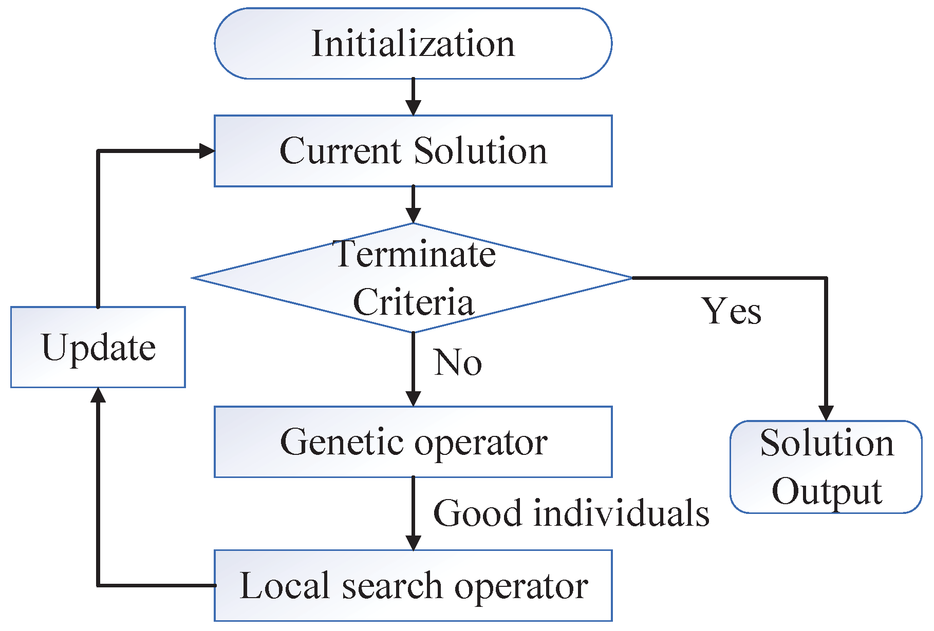
3.1. Algorithm Principle

The traditional location–allocation problem in a two-level hub-and-spoke network has proven to be Non-deterministic-Polynomial (NP)-hard in many references [26,29], implying that the problem cannot be solved in polynomial time. The mathematical model in this paper was developed by extending the two-level hierarchical network structure to a more-complicated three-level hierarchy. Meanwhile, the objectives of UTM service users (i.e., the UAS) and suppliers were jointly combined in the optimization model, which makes the route network design problem even more challenging to solve. Therefore, heuristic algorithms such as the Genetic Algorithm (GA) and Simulated Annealing (SA) were jointly adopted and improved in this work to incorporate the advantages of both global and local searches.

SA is a local search algorithm that simulates the physical annealing in metal processing [30]. As one of the simplest and best-known metaheuristic methods, SA is widely deployed for a near-optimal solution search in NP-hard problems. However, the algorithm needs a substantial amount of computing time since it generally follows a single search thread at a time. To enhance the search capability, a hybrid Simulated Annealing Genetic Algorithm (HSAGA) is proposed with the principle as follows. The GA will simultaneously search different solution regions thanks to its population-based nature. For those good individuals provided by the GA, their neighborhoods will be probabilistically searched according to the SA-based solution acceptance criterion. The framework of the HSAGA is given in Figure 2. After the hybridization of the global genetic operator and local search operator, the algorithm proceeds to update the solution population and iterates the procedure until the termination criterion is satisfied.

Within the HSAGA framework, decision variables of the UAS route network design problem are encoded to construct a solution chromosome, which can be further divided into two stages. In the first stage, a two-layered chromosome encoding is used to determine the location and number of the primary and secondary sites. In the second stage, a site allocation scheme is generated to determine the allocation relationships between ordinary (secondary) sites and secondary (primary) sites. In short, detailed chromosome construction is described by the process diagram shown in Figure 3.

As depicted in the sampled chromosome in Figure 3, the first layer is an unrepeated sorting of all demand site indicesin the airspace, which indicates the chances of sites becoming high-level sites (e.g., site 5 has the highest probability of being selected as the primary site in this case). The second layer is an integer array (denoted as M) representing the number of primary and secondary sites. For instance, if $M=[3,4]$, it indicates that the first three sites (e.g., 5, 8, and 9 in red color) are assigned as primary sites, and the other four sites (e.g., 4, 7, 10, and 12 in blue color) are assigned as secondary sites. The site-allocation scheme indicates the allocation relationships among sites of different hierarchies, i.e., if a low-level site is allocated to a high-level site k, the numerical value corresponding to its position is k. In this case, primary site 1 is allocated to secondary site 4. Thus, the first position in the site allocation scheme is 4. In the following subsections, how the HSAGA finds the optimal solution chromosome will be described.

3.2. Genetic Operator

As mentioned before, the global search process is executed by the population-based search algorithm, the GA, due to its huge solution search regions. Theoretically, the GA will not be confined to any particular search space if the population pool includes sufficient candidates, and new diversified genes will be introduced during the process. For new population creation, three genetic operators, select, cross, and mutate, are used in the global search:

• Select: The tournament selection strategy is applied to ensure that the fittest candidates from the current generation are passed on to the next generation.
• Cross: The single-point crossing strategy is used by randomly selecting the same position on two parent chromosomes. Then, the genetic information to the left (or right) of this point is swapped between the two parents to produce offspring chromosomes. Yet, it is worth noting that two parts of the information are contained in the chromosome: the site hierarchy and the allocation relation. If two chromosomes are randomly crossed, the new chromosomes may not have practical significance. Therefore, after the single-point crossover process is completed, check whether each newly generated offspring meets the topology constraints and, then, make appropriate adjustments to the new offspring.
• Mutate: The single-point variation is adopted if the mutation probability is satisfied. Randomly select a chromosome as the parent, and modify its gene to a new value under the topology constraints.

3.3. Local Search Operator

As promising complements to global search, local search is then applied to good individuals generated by the above three genetic operators. Seeking to improve the current solution by making incremental changes, two local search operators are specifically designed to explore the neighborhood solutions of the good individuals.

To start with, the centrality measures derived from graph theory are firstly introduced. Their notations are summarized and explained in

Table 3. Basic centrality notations and explanations.

Notations	Explanations
$Cluste{r}^m$	Cluster of secondary and ordinary sites that are attached to one same primary site m,
	$m\in \mathcal{A}$
$h\left[i\right]$	=m if site i belongs to $\mathcal{C}luste{r}^m$ and is either directly ($i\in \mathcal{H}$) or indirectly ($i\in \mathcal{O}$)
	attached to primary site $m,m\in \mathcal{A}$
$c_{in}\left[i\right]$	Internal closeness of site i, $i\in \mathcal{D}$
$c_{ex}\left[i\right]$	External closeness of site i, $i\in \mathcal{D}$
$w_{in}\left[i\right]$	UAS traffic volume entering site i, $i\in \mathcal{D}$
$w_{out}\left[i\right]$	UAS traffic volume leaving site i, $i\in \mathcal{D}$

. Given a candidate location–allocation solution chromosome, all secondary and ordinary sites that are attached to one common primary site comprise a cluster. That is, $h\left[i\right]=h\left[j\right]=m$ indicates that sites i and j belong to the same cluster $Cluster{}^m$. The primary site with the same site index assigned to it ($h\left[m\right]=m$) is the center of the cluster. For clusters in the route network, two types of site closeness are defined as follows:

$$c_{in}\left[i\right]=\frac{1}{{\sum }_{h\left[i\right]=h\left[j\right]}{L}_{e(i,j)}},c_{ex}\left[i\right]=\frac{1}{{\sum }_{h\left[j\right]=j}{L}_{e(i,j)}}$$

(12)

where $c_{in}\left[i\right]$ and $c_{ex}\left[i\right]$ are the internal closeness and external closeness of site i, respectively. The internal closeness can be described as the inverse of the sum of the distance from site i to all other sites that are in the same cluster, and the external closeness is characterized as the inverse of the sum of distance to all other cluster centers.

Based on the closeness measures, two local search operators, i.e., swap and reallocate, are specifically designed to generate neighbor solutions that have high opportunities to be accepted:

• Swap: Hierarchies of two demand sites within the same cluster (one site is allocated to the other) are swapped according to their $V_{swap}$ values. For instance, if a primary site and a secondary site are selected, compare their $V_{swap}$ values. Then, the primary site with a lower $V_{swap}$ value becomes a secondary site, while the previous secondary site with a higher $V_{swap}$ value is changed to be the primary site.

  $$V_{swap}\left[i\right]=c_{in}\left[i\right]·c_{ex}\left[i\right]·(w_{in}\left[i\right]+w_{out}\left[i\right])$$

  (13)

  where $w_{in}\left[i\right]$ and $w_{out}\left[i\right]$ are the UAS traffic volume that enters site i or leaves it, respectively.

  $$w_{in}\left[i\right]=\sum _{w\in \mathcal{W}}\sum _{j\in \mathcal{D}}{\delta }_{e(j,i)}^w·d_w,w_{out}\left[i\right]=\sum _{w\in \mathcal{W}}\sum _{j\in \mathcal{D}}{\delta }_{e(i,j)}^w·d_w$$

  (14)
  In principle, the swap operator tries to raise the hierarchy of a site on the condition that: (1) its closeness to other sites in the cluster is high; therefore, it can reduce the total costs of collection and distribution within the cluster; (2) its closeness to other clusters is high; therefore, it can reduce transfer costs; (3) the total amount of the traffic demand that enters it or leaves it is large enough.
• Reallocate: the non-primary site with the largestvalue of $V_{reallocate}$ is selected and reallocated to one of the other clusters.

  $$V_{reallocate}\left[i\right]=c_{ex}\left[i\right]/c_{in}\left[i\right]$$

  (15)
  In other words, the reallocate operator aims to detach sites that are far from other sites in the same cluster, but close to other primary sites. Although the reallocate operator will not necessarily achieve the best site allocation, it ensures that sites with a close distance to each other are placed in one cluster.

As a result, critical sites with high values of $V_{swap}$ and/or $V_{reallocate}$ are chosen for participation in the local search operations of swap and reallocate, which will noticeably reduce the search space and improve the solution quality.

3.4. Solution Updating

To utilize the maximum benefits of the global and local search hybridization, two main issues need to be handled beforehand. The first issue is the intensity of local search, which controls the maximum computational budget spent on improving one certain good solution. In order to avoid premature convergence and reduce resource waste at the same time, the local search intensity should adapt to the search status and change dynamically. The second issue is to establish an appropriate acceptance criterion for the multi-objective problem, which decides about whether to accept a newly generated solution or not. Therefore, with particular emphasis on the above two issues, how to update the solution is discussed in this subsection, where the intensity of the local search is guided by SA and a weighted vector is used to make acceptance decisions for two conflicting objectives.

Inspired by the annealing procedure in metallurgy, the local search intensity of the proposed algorithm varies with an SA function. Once the initial annealing temperature and reduction factor are determined, the deepness of the local search gradually grows along with the decrease of the temperature. That is, a neighborhood solution will be accepted quickly at the beginning of the local search with a low searching accuracy (i.e., accept a temporarily worse solution according to the Metropolis criteria). When the temperature goes down to approach the lowest limit, the intensity will be increased in the elite searching area to improve the solution quality. The details of the SA-based local search intensity implementation are indicated in Algorithm 1.

Algorithm 1 Pseudo-code of the HSAGA.

1: Input: set of demand sites $\mathcal{D}$, UAS OD pairs $\mathcal{W}$, population size $\mu$, maximum generation $MaxGen$ 2: % to initialize the chromosome population $Pop\left(0\right)$ 3: set chromosome index $l=1$, generation $g=0$ 4: while $l\le \mu$ do 5:    randomly construct a solution $Po{p}_l\left(0\right)$ 6:    if all topology constraints satisfied, then 7:       $l+=1$ 8:    end if 9: end while 10: % of main procedure 11: while $g<MaxGen$ do 12:    % to apply global genetic operator to $Pop\left(g\right)$ 13:    $Po{p}^{\beta }\left(g\right)\leftarrow select,cross,mutate\left(Pop\left(g\right)\right)$ 14:    % to apply local search operator to good individuals in $Po{p}^{\beta }\left(g\right)$ 15:    set initial temperature $T=T_0$, reduction factor $\kappa$, predefined $T_{end}$, weighted vector $\mathbf{\lambda }$ 16:    repeat 17:       generate a random number $\zeta ,0\le \zeta \le 1$ 18:       if $\zeta <0.5$, then 19:          $Po{p}^{\gamma }\left(g\right)\leftarrow swap\left(Po{p}^{\beta }\left(g\right)\right)$ 20:       else 21:          $Po{p}^{\gamma }\left(g\right)\leftarrow reallocate\left(Po{p}^{\beta }\left(g\right)\right)$ 22:       end if 23:       % to apply solution updating 24:       $\Delta =fit(\mathbf{\lambda },Po{p}^{\gamma }\left(g\right))-fit(\mathbf{\lambda },Po{p}^{\beta }\left(g\right))$ 25:       if $\Delta <0$, then 26:          accept $Pop(g+1)\leftarrow Po{p}^{\gamma }\left(g\right)$ 27:       else 28:          accept $Pop(g+1)\leftarrow Po{p}^{\gamma }\left(g\right)$ with probability $exp(-\Delta /T)$ 29:       end if 30:       $T=\kappa ·T$ 31:    until $T<T_{end}$ 32:    g+=1 33: end while 34: Output: final population $Pop\left(g\right)$ of site location–allocation in hierarchical UAS route network

For single-objective optimization, the objective function itself is the fitness evaluation criterion that determines the acceptance of a neighborhood solution. However, things are quite different in multi-objective optimization. Using the weighted sum method, a weighted vector defined as $\mathbf{\lambda }=[{\lambda }_1,{\lambda }_2]$ is adopted to combine the two normalized objectives into one single fitness function.

$$fit(\mathbf{\lambda },Po{p}_l)=\sum _{m=1}^2{\lambda }_m\frac{Ob{j}_m\left(Po{p}_l\right)-Ob{j}_m^{min}}{Ob{j}_m^{max}-Ob{j}_m^{min}}$$

(16)

where ${\lambda }_1=rand(0,1)$, ${\lambda }_2=1-{\lambda }_1$ are randomly updated. $Ob{j}_m^{min}$ and $Ob{j}_m^{max}$ are the minimum and maximum objective values in the current population $Pop$, and the individual l of $Pop$ is denoted as $Po{p}_l$.

Finally, the complete pseudo-code is demonstrated in Algorithm 1 to present a full picture of the HSAGA’s implementation.

4. Result and Discussion

In this part, the established hierarchical UAS route network model is applied in Beijing region of China, where optimal location–allocation is determined in accordance with UAS air travel demand. Numerical results are obtained using the MATLAB R2017b software running on a PC with an Intel Core i5 5200U CPU 2.19 GHz processor.

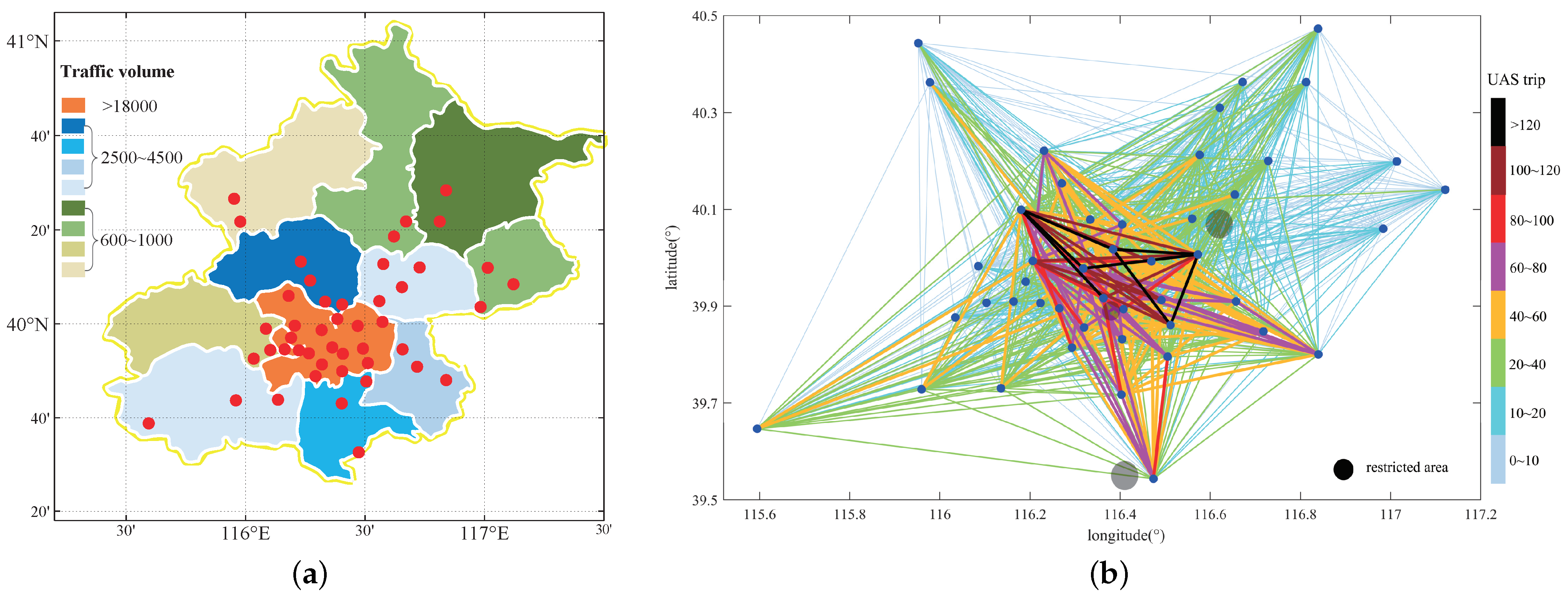
4.1. Simulation Design

The research area in Figure 4a corresponds to the administrative region map of Beijing and includes 16 districts. As exact UAS travel demand data are not available for current use and, also, the existence of multi-modal transportation may complicate the travel behavior, a numerical study was randomly generated in this paper based on the Beijing Sustainable Urban Transport project [31]. In total, 20,141 trips were estimated to occur to and from 46 potential demand sites, the distribution of which would be assigned according to social and economic attributes. The corresponding UAS trip distribution in the research region is depicted in Figure 4b with edges colored differently to represent the varying degrees of the trip volume. Tenser UAS traffic demand is labeled with a darker edge. Edges whose trip volumes are over 120 are marked with black, while volumes within the range of [100, 120], [80, 100], [60, 80], [40, 60], [20, 40], [10, 20], and [0, 10] are colored in brown, red, pink, yellow, green, blue, and light blue, respectively. Specifically, three restricted areas (shaded in light black for illustration) are designated in the central, southern, and northeastern parts of the region map, where UASs are prohibited from flying over (e.g., government, airport).

As shown in the figure, the UAS demand distribution demonstrates an obvious spatial aggregation from the suburbs to the urban core. Besides, it should be noted that only trips longer than 10 mi of direct distance are tested as UAS travel candidates in the figure. Trips shorter than this would be less appealing to UAS flights since the driving option would be more preferable. Other parameters used in the numerical study are presented in

Table 4. Parameter settings.

Parameter	Value
UAS cruise speed (mi$·{\mathrm{h}}^{-1}$)	150
Detour penalty $\gamma$	1.2
Maximum number of primary sites $N_1$	8
Maximum number of secondary sites $N_2$	12
Discount rate in main route $\alpha$	0.65
Discount rate in trunk route $\beta$	0.75
Resource quantity per primary site $R_m$	100,000
Resource quantity per secondary site $R_a$	50,000
Length restriction on site allocation $R_{max}$ (mi)	60
Population size $\mu$	30
Maximum generation $MaxGen$	150
Crossover probability $p_c$	0.65
Mutation probability $p_m$	0.05
Initial temperature $T_0$ (${}^{°}$C)	100
Cooling factor $\kappa$	0.98
Final temperature $T_{end}$ (${}^{°}$C)	0.2

.

Specifically, the parameters of the global genetic operators in the HSAGA were well-tuned according to the sensitivity analysis shown in Figure 5, where a small test case (20 sites and 6500 UAS travels involved) was conducted to ensure that the experimental performance was achieved with the best parameters. The overall solution optimality was assessed by the hypervolume indicator IH, and the optimal crossover probability $p_c$ and mutation probability $p_m$ that led to the highest IH were selected. Owing to its broad applicability, the parameters of the SA-based local search were set as the default [32].

In the following context, a detailed experiment will be conducted together with benchmark instances to verify:

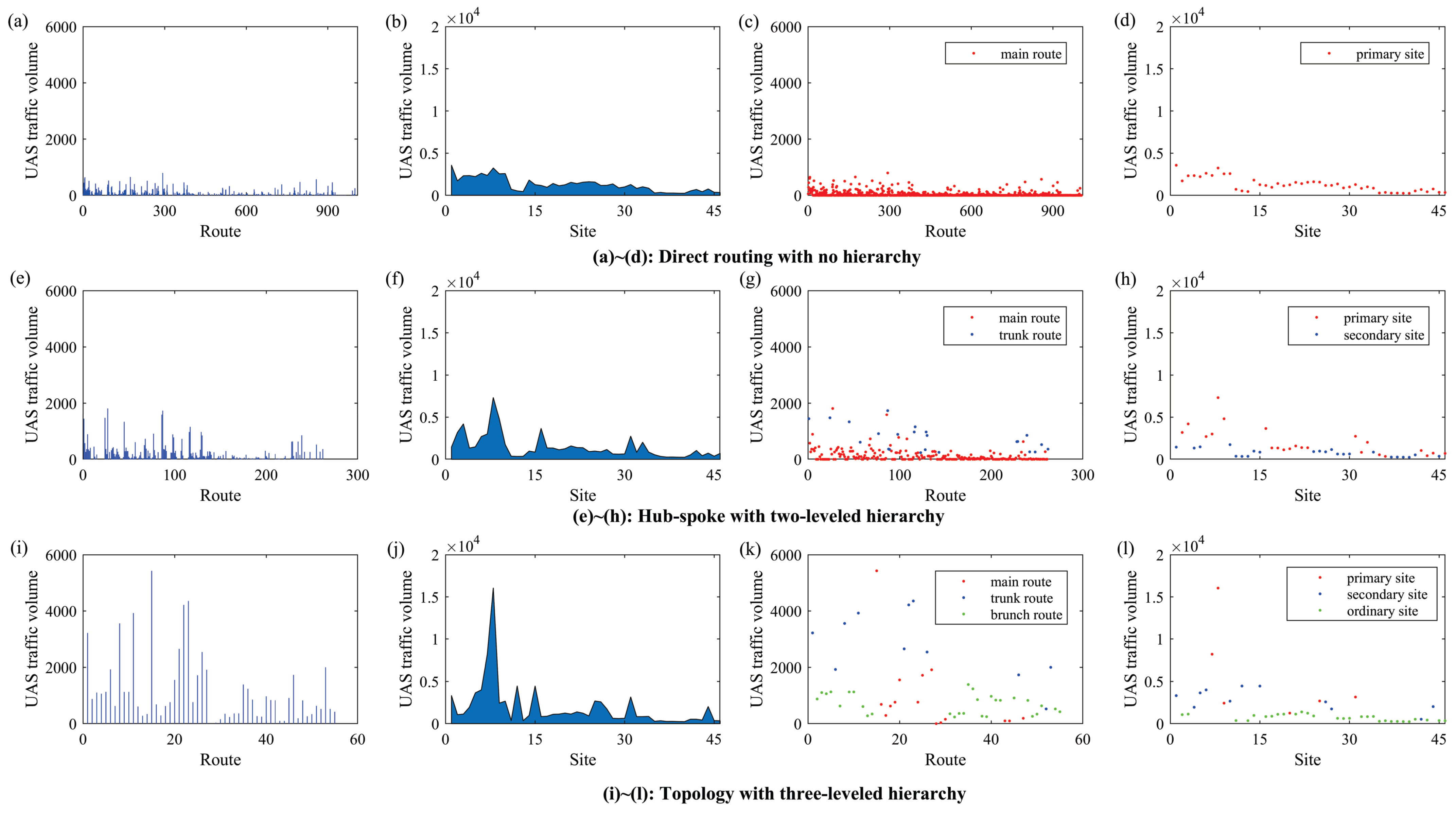
• The effectiveness of the three-level hierarchical structure: (1) direct routing (no hierarchy), (2) hub-and-spoke (two-level hierarchy), and (3) the proposed hierarchical topology (three-level hierarchy).
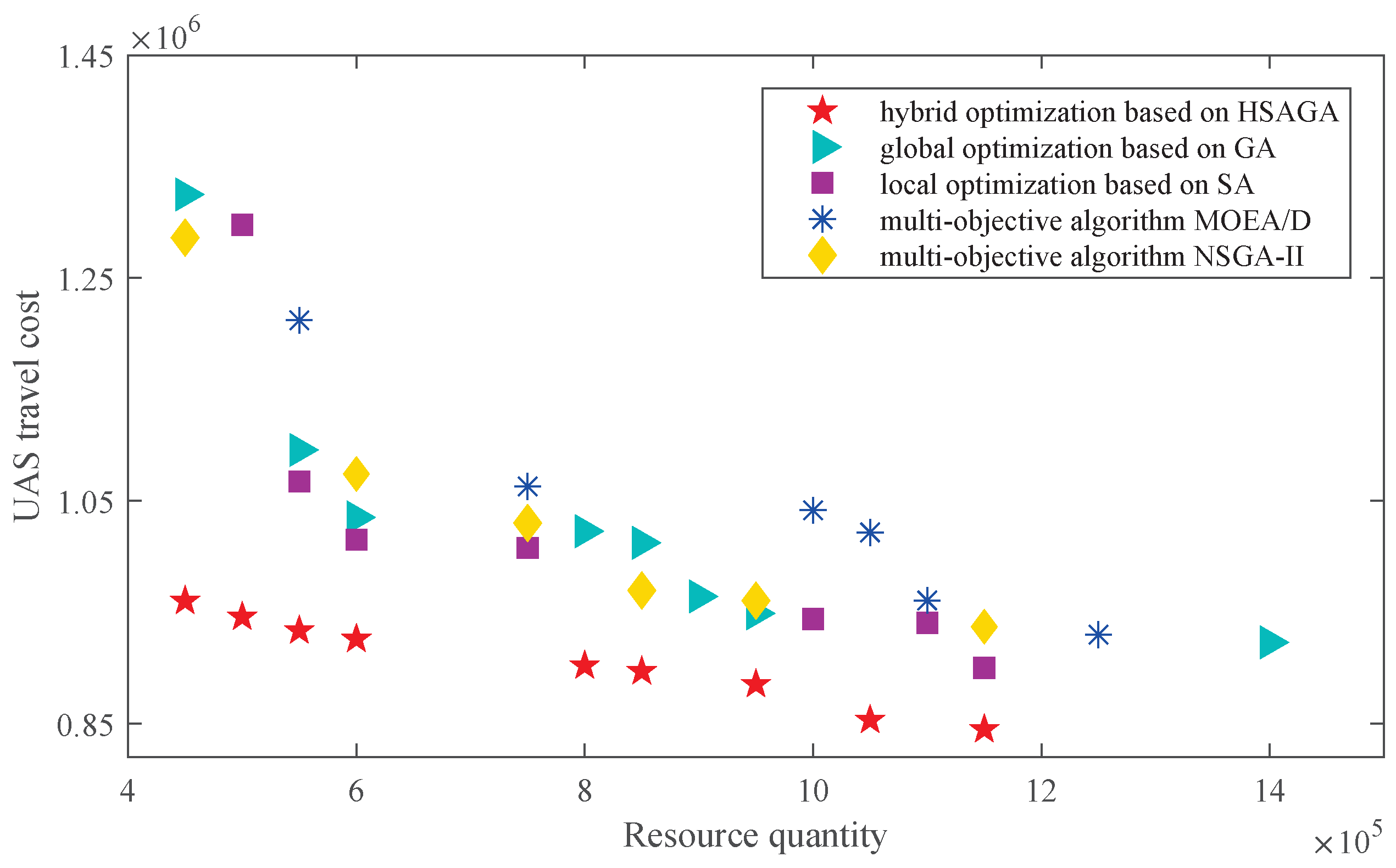
• The effectiveness of the global–local hybridization strategy: (1) pure global optimization based on the GA, (2) pure local optimization based on SA, and (3) the proposed hybrid global–local optimization based on the HSAGA.
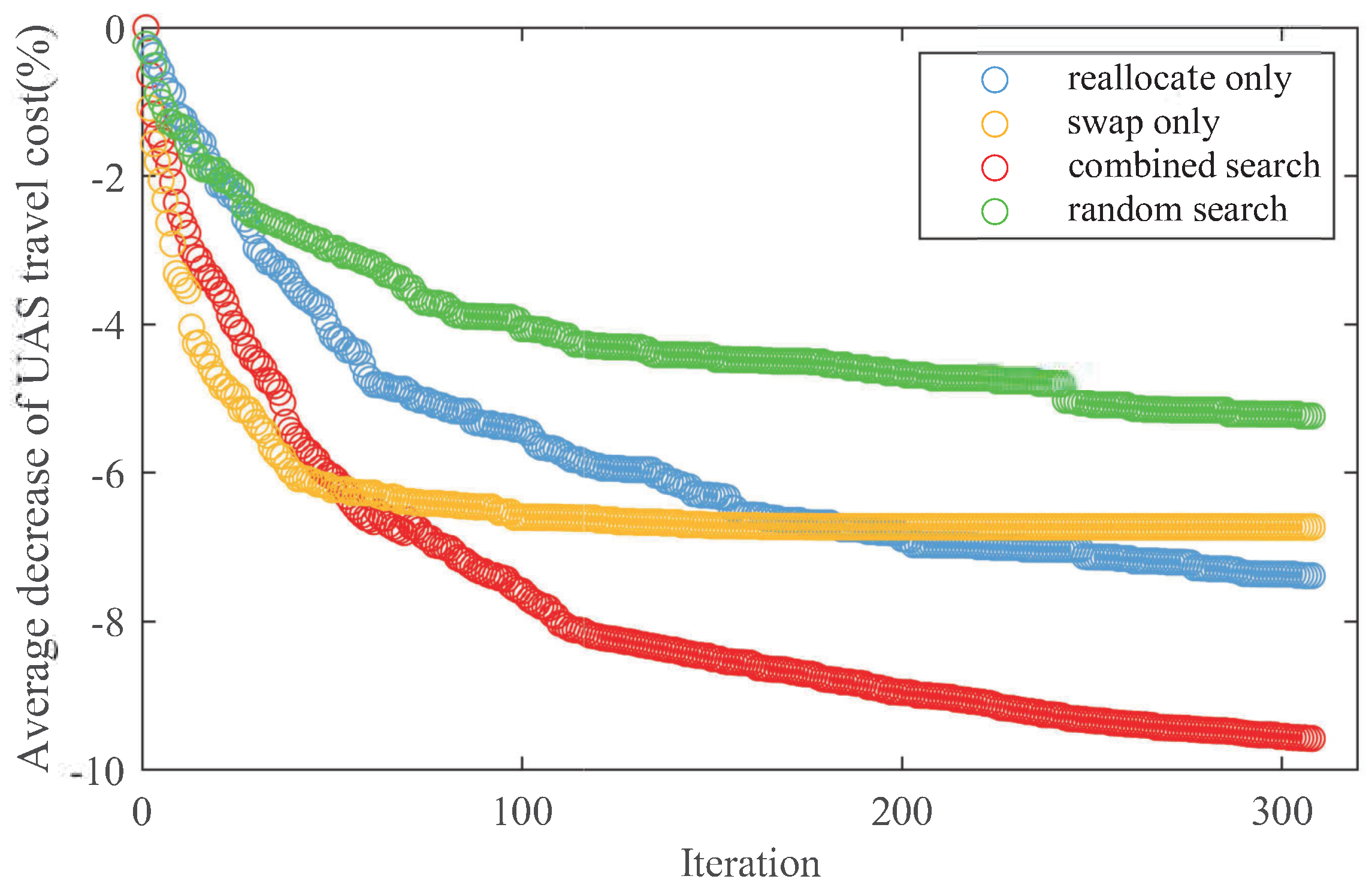
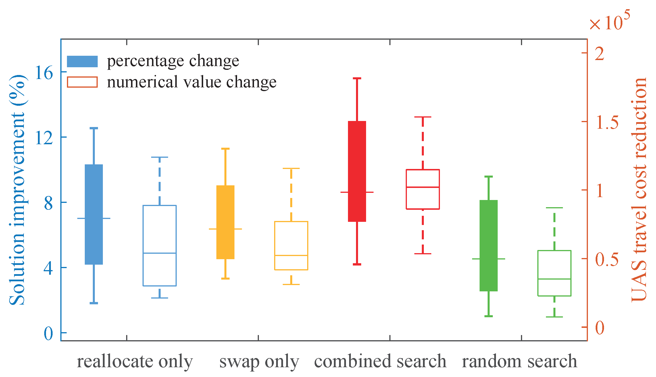
• The effectiveness of the problem-specific local search operator: (1) random search, (2) swap-only operator, (3) reallocate-only operator, and (4) combined search with both swap and reallocate operators.
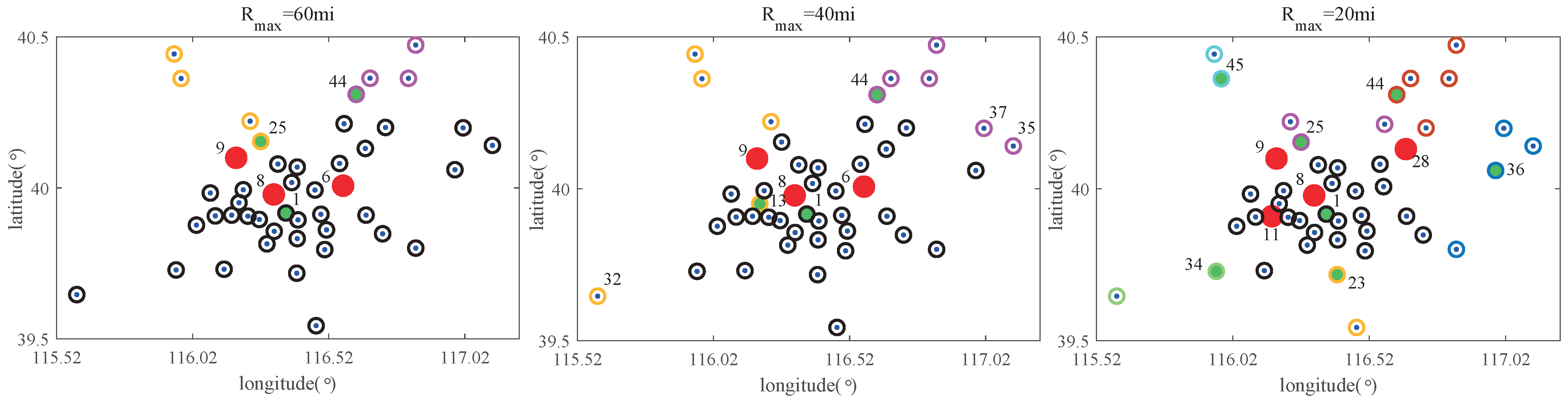
• The sensitivity analysis of critical parameters: the length restriction on site allocation $R_{max}$.

For each simulation, the results were collected and analyzed on the basis of 10 independent runs.

4.2. Validation of the Three-Level Hierarchy

The performance of the network hierarchy was firstly analyzed by comparing the average result of the direct routing network and the hierarchical routing network in

Table 5. Comparison of direct routing network and hierarchical routing network.

Mode of Network	Number of Sites			Number of Routes			UAS Travel Cost	Resource
	Primary	Secondary	Ordinary	Main	Trunk	Branch	(Million)	(Million)
direct routing with no hierarchy	46	-	-	1005	-	-	0.52	4.60
hub-and-spoke with two-level hierarchy	24.75	21.25	-	345.88	21.25	-	0.61	3.54
topology with three-level hierarchy	4	7.33	34.67	6.56	7.33	34.67	0.90	0.77

. Unlike the direct routing network, where all demand sites are fully connected, most of the UAS trips in the hierarchical network need to be transferred intermediately to high-level sites rather than travel directly to their destinations. From the table, one can observe that the network cost in direct routing network was about 5.12 million, where the UAS travel costs and resource quantities accounted for about 10.16% and 89.84% of the total cost, respectively. By adopting the hierarchical network structure, the UAS travel cost increased slightly as the resource quantity substantially decreased, i.e., 1.06 million less in the two-level hierarchy and 3.83 million in the three-level hierarchy. That is because the hierarchical topology allows infrastructure savings (e.g., fewer high-level sites and routes) as it permits a more-concentrated utilization of resources. Instead of building massive direct routes, less-frequent UAS travel demands can be served by transferring to high-level sites. Compared to the total costs of the direct routing network and hub–spoke network, our three-level model saved 67.38% and 59.76% of the costs, respectively.

Considering that some network properties (e.g., UAS traffic volume distribution in routes and sites) are case-sensitive and cannot be averaged, we took one concrete sample for each mode of network in Figure 6 to illustrate the traffic routing process in detail.

From these experimental results obtained in Figure 6 and Table 5, we can have the following observations: (1) Unlike the direct routing network containing 1005 route segments in Figure 6a, the sampled two-level hub–spoke network contains 262 segments in Figure 6e, and the total number of routes for the three-level route network is 55 in Figure 6i. As the number of air routes decreases, the uneven distribution of UAS traffic among network routes becomes evident. For instance, certain routes experience intense traffic volumes, while others remain comparatively sparse. (2) Similarly, there is also considerable heterogeneity in the UAS traffic volume among the 46 demand sites in Figure 6b,f,j. This occurs because of the reduction in route redundancy, i.e., several demand sites serve as central points for various OD pairs and attract a greater traffic concentration compared to other sites. (3) When considering the route category, the increase in network levels generates an obvious role disparity. For instance, compared with Figure 6c,g, where the UAS traffic carried by routes of different categories (denoted by different colors) exhibits little difference, the main and trunk routes make up 47% of the three-level route network in Figure 6k, but carry 80% of the UAS traffic volume. (4) Such a role disparity is also found in the demand site categories in Figure 6d,h,l. For instance, the peak volume reaches 16,000 at the primary sites in Figure 6l, while being generally below 2000 at the ordinary sites. Therefore, benefiting from higher network resource utilization (i.e., the average UAS load per route was 38 in the direct routing network, 171 in the two-level route network, and 1183 in the three-level route network), the results verified that a high-quality hierarchical route network model could help to meet the UAS traffic demands, as well as simplify the network layout.

For a further analysis of the three-level network hierarchy, Figure 7 provides an instance of optimal site location–allocation with 6 primary sites and 11 secondary sites in the network. Primary sites are represented by red nodes, secondary sites by green, and ordinary demand sites by blue. We also present how UAS traffic flows are routed in the figure (light blue: flow volume <1000, orange: ≥1000 to <2000, pink: ≥2000 to <3000, black: ≥3000). The results showed that the largest volume of traffic mainly concentrated in the main routes and trunk routes. Specifically, it was found that the main routes connecting primary sites do not always carry the busiest UAS traffic (for instance, some main routes between two remote primary sites are colored in light blue). Instead, some trunk routes connecting the primary site and secondary site have greater traffic loads, suggesting that most UAS trips transfer to only one intermediate primary site rather than two.

To explore the influence of UAS non-direct routing on the above hierarchical route network in Figure 7, Figure 8 gives the distribution of the additional travel distance compared to point-to-point routing. Extra UAS travel cost due to intermediate transfer is inevitable in the hierarchical route network for routing some flows via their non-shortest paths. It can be seen from the figure that approximately 75% of the UAS trips had an extra travel distance of less than 10 mi. On average, the additional distance was 7.38 mi, indicating an acceptable delay time of 3 min given that the UAS cruise speed is 2.5 mi/min.

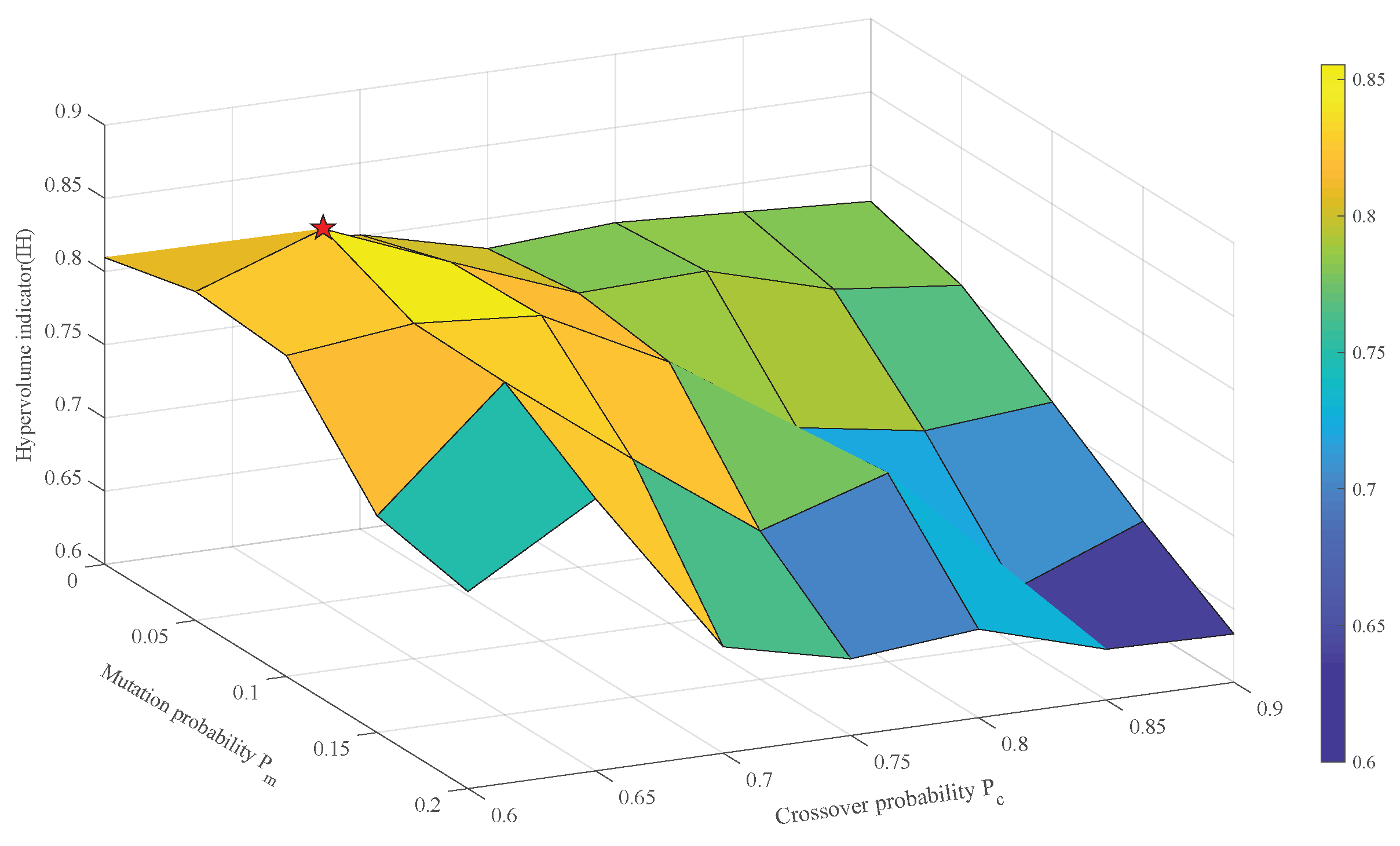
4.3. Validation of the HSAGA

From the first set of experiments, the superiority of the hierarchical structure was justified by a comparison with the traditional non-applied one. This section investigates whether the proposed HSAGA contributes to the success of such a network. Other optimization algorithms such as the GA and SA were employed and compared to demonstrate the effectiveness of the HSAGA. These algorithms differ in their search ability; for instance, the GA has a strong global search ability, and SA performs well in local search, which will have an impact on the optimization results. To further verify the effectiveness of the proposed HSAGA in multi-objective UAS route network design, two typical state-of-the-art algorithms, NSGA-II and MOEA/D, were also considered for the comparison studies. NSGA-II relies on non-dominated sorting and crowding distance, while the working principle of MOEA/D is a decomposition strategy. Figure 9 depicts the non-dominated solutions of the five compared algorithms, where no one objective function can be improved in a non-dominated solution without degrading the other objective value.

We can see that the HSAGA with the global and local search combined outperformed the other algorithms in terms of the UAS travel cost and network resource quantity. This is because the single-mode search algorithm only focuses on one kind of search option and, thus, is more likely to run into partial optimization. For the two state-of-the-art algorithms, NSGA-II and MOEA/D, NSGA-II provided comparatively superior solutions due to its elitism, which preserves the best solutions over successive generations, while MOEA/D experienced premature convergence due to the sensitivity to the weight configurations. Apart from the fact that the GA and SA have been extensively adopted for their proven effectiveness, the superiority of the HSAGA is driven by the following considerations. Unlike the single-mode search algorithm, which only focuses on one kind of search option, the HSAGA strikes a balance between global exploration and local exploitation. For the GA-based global optimization, promising solutions in the large solution space ($3(n\ast (n-1)/2)$ in this case) can be approximated from multiple points through iterative selection, crossover, and mutation. For example, offspring that differ from existing parent chromosomes are reassembled during the crossover process by randomly breaking and re-joining the parent genetic information. Therefore, solutions with various travel costs and resource quantities can be gradually evolved. In the meantime, in case the solution of the GA is trapped at its current local minima, the SA-based local optimization can avoid early convergence by probabilistically accepting bad neighborhood solutions. For example, the hierarchies of two sites can be reassigned and allocation relations can be relinked by reallocating a selected site to other sites, the intensity of which is naturally controlled by the temperature, which can prioritize exploration initially and transition to exploitation as the optimization progresses. Specifically, it should be noted that only the UAS travel cost was improved, while the resource quantity remained the same during the local search, since the numbers of primary and secondary sites needed to be constructed were unchanged after the optimization. However, one drawback of local optimization is its strong dependence on the initial solution, i.e., solution diversity will be rare because the local search always operates on the same individual constantly.

Unlike single-mode search algorithms, the proposed HSAGA jointly combines the global search of the GA and the local search of SA. In this case, the result generated by the GA is regarded as the initial solution of local optimization so as to avoid premature convergence. Meanwhile, the diversity in the GA population can be reserved in the local search process by keeping individuals with good qualities. Consequently, by reasonably hybridizing multiple search modes, the HSAGA promotes the probabilities of finding optimal site location–allocation solutions for the UAS route network. A quantitative comparison of four performance indicators (i.e., IH, ID, $\Delta$, and time) is given in

Table 6. The values of four performance metrics, IH, ID, $\Delta$, and time.

Optimization Strategy	Metric	IH	ID	$\Delta$	Time (Min)
global optimization based on GA	mean	0.649	0.016	0.641	92.48
	std	0.017	0.010	0.110	2.95
	best	0.671	0.009	0.550	90.45
local optimization based on SA	mean	0.659	0.026	0.670	88.10
	std	0.013	0.003	0.059	3.82
	best	0.666	0.018	0.632	84.21
hybrid optimization based on HSAGA	mean	0.897	0.013	0.606	111.03
	std	0.015	0.004	0.079	3.48
	best	0.911	0.006	0.499	105.69
multi-objective optimization based on MOEA/D	mean	0.630	0.033	0.703	103.68
	std	0.012	0.006	0.100	3.09
	best	0.677	0.021	0.600	92.00
multi-objective based on NSGA-II	mean	0.708	0.019	0.479	120.95
	std	0.042	0.009	0.161	3.64
	best	0.744	0.007	0.338	113.07

, including the best result for each indicator and the corresponding standard deviation.

The first three indicators were adopted to measure the solution quality, where the hypervolume indicator IH implies the size of the dominated space, the convergence indicator ID represents the proximity to the reference set, and the diversity indicator $\Delta$ reflects the distribution of non-dominated solutions. We can conclude from Table 6 that the HSAGA-based hybrid optimization was the superior one, which had the largest IH, while the smallest ID and a moderate $\Delta$. The quantitative comparison was also consistent with the algorithm’s working principle mentioned before, as the diversified population generated from the global search and the following local search provided greater chances of approaching the optimal network layout configuration. The forth indicator implies the computational efficiency of the HSAGA. One can see that local optimization based on SA was slightly more efficient than the global optimization based on the GA. This was mainly because the global optimization used three genetic steps (i.e., select, cross, and mutate) for generating new solutions, while the local optimization used a single step (i.e., swap or reallocate). In addition, when a chromosome is generated by genetic optimizations, we usually have to check whether the new solution complies with the predefined constraints, while the local optimization always provides reasonable solutions. Therefore, for the sake of computation time, the HSAGA only applies local search to non-dominated individuals instead of to every solution in each generation.

Next, in order to give a comprehensive evaluation of how the problem-specific local search operators were working, the average values of the UAS travel cost decrease to the evolution of iterations are plotted in Figure 10. The declining curves illustrate that the combined search can achieve a greater cost reduction than the single local search and random search, which possesses no local search operator. With the same initialization, the swap-only local search sped up the convergence process, but the premature convergence problem emerged around 100 iterations. This is because the swap operator does not change the site combinations within each cluster and, thus, may be easily trapped in local minima. In contrast, the reallocate operator searched a broader solution space with changed site combinations among different clusters, enabling a higher chance for finding new potentially cost-effective solutions. Therefore, by incorporating both the swap and reallocate operators, the combined local search worked well, finding high-quality solutions and avoiding premature convergence. Improvements in the solutions after local searching (i.e., less UAS travel costs with the same number of high-level sites constructed) across 10 independent runs are depicted in Figure 11. The performance enhancement was measured both in percentage terms and in numerical values, which are represented by filled and hollow boxplots, respectively.

One can see that the combined search had the most-satisfying best and average function values compared to those of the other three search strategies. The relative decrease of the UAS travel cost was on average 7.0% in the reallocate-only neighborhood search, 6.7% in the swap-only neighborhood search, 9.7% in the combined search, and 5.2% in the random search. As a typical NP-hard problem, the search space for optimal site location–allocation is too large to approximate a promising result. Unlike the random search operator searching all the solution space blindly, the swap and reallocate search operators guide the search process to elite feasible regions, where the former one focuses on changing the site hierarchy within the same cluster and the latter tends to adjust the site allocation relations across different clusters. Hence, the solution quality was considerably improved by the precise neighborhood search.

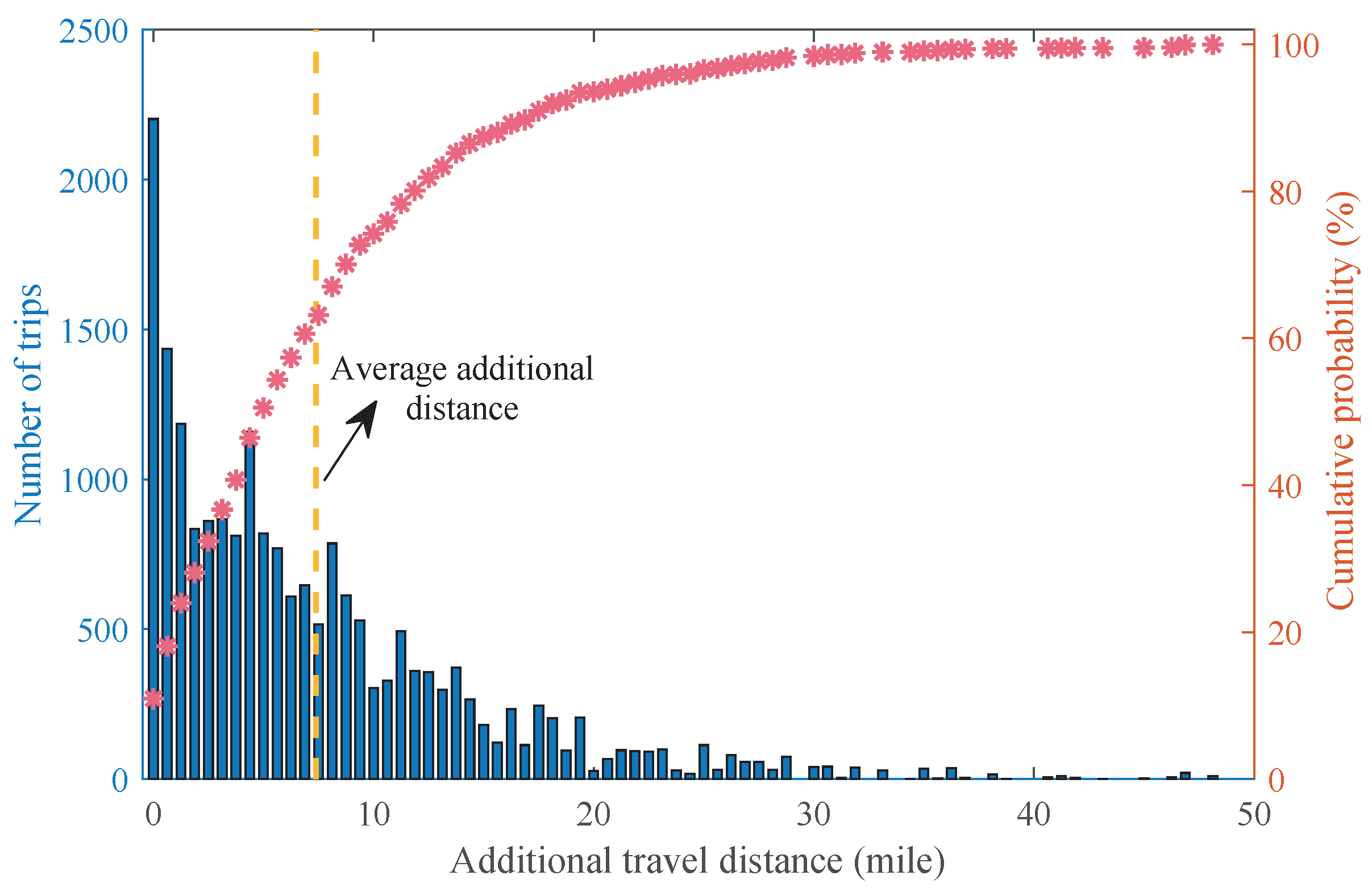
4.4. Sensitivity Analysis of Critical Parameter

To understand how some critical parameter settings may influence the route network layout and UAS routing behavior, a sensitivity analysis of the length restriction $R_{max}$ on site allocation was also carried out. As an important network parameter, the range restriction on the route distance between two connected demand sites must be satisfied according to the UAS endurance requirements. In the original experiment, the length restriction $R_{max}$ was set to 60 mi. Next, on the premise of keeping network connectivity (there were routes connecting any given UAS OD pair across the network), we changed the length restriction to $R_{max}$ = 40 mi and $R_{max}=$ 20 mi. Figure 12 depicts the optimal network layout that requires the least resource quantity under three different length restrictions. Red nodes represent primary sites; green nodes with outer colored rings represent secondary sites; blue dots represent ordinary sites that are allocated to the corresponding secondary sites with the same outer ring color.

In general, $R_{max}$ implicitly clustered demand sites in terms of their geographical distance and, thus, demonstrated the characteristic of spatial aggregation, i.e., ordinary sites that were close in distance tended to be allocated to the same secondary site. This allows UAS traffic to travel much more efficiently with fewer intermediate stops. For instance, for a short-haul flight, only one intermediate stop is needed if the origin and destination sites are allocated to the same secondary site, while three stops at least are required if they are allocated to two separate secondary sites. When the allocation threshold was decreased to 40 mi, the backbone structure remained unchanged, but the previous secondary site 25 was replaced by site 13. This is because dispersedly located ordinary sites, such as 32, 35, and 37, require reallocations to closer secondary sites that are within their allocation limits. However, a further decrease of $R_{max}$ to 20 mi resulted in a significant topology change. The number of primary and secondary sites increased from 3 to 4 and 7, respectively. That is, more high-level sites were constructed for the purpose of intermediate transfer, given that a greatly reduced allocation threshold makes the network connectivity more difficult to preserve. Indeed, network connectivity no longer existed when the allocation limit was less than 20 mi as some dispersed sites will be disconnected.

Apart from the network layout demonstration in Figure 12, the detailed properties of these sampling networks are also recorded in

Table 7. Network properties under different $R_{max}$.

Property	${\mathit{R}}_{\mathbf{max}}$ = 60 mi	${\mathit{R}}_{\mathbf{max}}$ = 40 mi	${\mathit{R}}_{\mathbf{max}}$ = 20 mi
Primary site No.	3 (6/8/9)	3 (6/8/9)	4 (8/9/11/28)
Secondary site No.	3 (1/25/44)	3 (1/13/44)	7 (1/23/25/34/36/44/45)
Resource quantity (mill.)	0.45	0.45	0.75
UAS travel cost (mill.)	0.96	1.00	0.97
Additional distance (avg.)	7.64 mile	8.75 mile	10.78 mile

. Compared with that of $R_{max}=$ 60 mi, more UAS travel costs were consumed in $R_{max}=$ 40 mi due to the increase in the additional traveling distance. For $R_{max}=$ 20 mi, the extra travel cost induced by the traveling distance extension was compensated by the service discount factors $\alpha$ and $\beta$. That is, when 4 primary sites and 7 secondary sites were constructed, benefits from service discounts in the main routes and trunk routes will offset the longer distance costs induced by multiple intermediate transfers.

4.5. Discussion

In this research, to better address future unprecedented low-altitude UAV management issues, we advocated the concept of hierarchical air route network construction. A typical three-level hierarchy was specifically adopted, i.e., UAS demand sites were categorized into primary, secondary, and ordinary sites, and route functions between pairs of sites were classified as the main route, trunk route, and branch route, correspondingly. The design of the UAS air route network was based on the demand distribution of the UAS traffic, and thus, air routes within the network will dynamically close and activate in response to changes in UAS traffic flow. In addition, the existing ground infrastructures such as buildings and other obstacles can be integrated into the route network structural design, which creates more logical routes and further enhances UAS traffic management.

UAS-oriented airspace utilization has gained increasing recognition in recent years, and various concepts of airspace structures have been proposed for using limited airspace as efficiently and safely as possible. The design of the public route network was firstly mentioned by ICAO at the Drone Enable, ICAO’s Unmanned Aircraft Systems (UASs) Industry Symposium in 2017, indicating that the industry considers this issue promising. Such a transportation concept is expected to achieve a more-concentrated airspace resource utilization, where one or more UAS flights can be assigned to fly along the shared routes. Specifically, by modeling the airspace as a three-level hierarchical route network, UAS traffic demands are addressed at multiple scales in accordance with the volume of traffic they accommodate (e.g., high-volume flow in the main route or local traffic supported by the branch route). In addition, based on the established route network, it is straightforward for UTM managers to identify the UAS flight situation and process UAS route allocation quickly in such a graph-type airspace structure.

UAS air route network design demands the support of a multi-objective optimization algorithm, which requires the maximization of the UAS transportation efficiency satisfying at the same time the network supplier concerns. If we explore the full combinatorial design space in detail, a large amount of computational resources will be needed. Therefore, a hybridization of global search with local search was adopted for the complex computation process, where the GA-based global search ensured that good solutions can be approximated from multiple points and the SA-based local search generated improved solutions on the basis of the solutions obtained by the GA. In the meantime, to overcome the computational load caused by the hybridization, only non-dominated individuals were chosen as initial solutions for the local search, where the swap and reallocate operators were applied for appropriate local search direction guidance.

In addition, it is essential to consider the sensitive impact of UAS endurance performance on the route network layout. As a harsh allocation length restriction would offset the economies of scale of traffic consolidation, future performance improvement in the UAS’s increasing range capability will contribute to the intensive design of the UAS route network.

5. Conclusions

This paper solved the multi-objective location–allocation optimization problem in the hierarchical UAS route network design. A three-level route network was used to model the transport hierarchy, where UAS demand sites were classified into primary sites, secondary sites, and ordinary sites and route functions were correspondingly classified as main routes, trunk routes, and branch routes. Specifically, in order to balance the interests between route system users and suppliers, the multi-objective decision-making framework was adopted to make a trade-off between UAS transportation efficiency and network construction efficiency. Meanwhile, a bi-level algorithm, the HSAGA, was designed for promising solution generation, where the advantages of the population diversity provided by the global search and local minima avoidance ensured by the local search were combined jointly. A case study in the Beijing region of China was carried out to verify the model and the algorithm. The results demonstrated that, compared to the direct routing network, a more-balanced transportation–construction trade-off can be achieved in a hierarchical UAS route network. Further simulations also confirmed the superiority of the proposed HSAGA, where the combination of the global and local search (conducted by two problem-specific operators) helped to find elite solutions more efficiently and precisely.

This study opens many future research directions. One possible improvement is that the current network only considers spatial design and does not relate to the temporal assignment of traffic routes between flights. As conflict risks are likely to increase in airspace where UAS traffic flows are concentrated, a deeper study with a time allocation strategy should be conducted to accommodate multiple UAS flights in the same routes at a particular time. Another direction is to incorporate the environmental impact into UAS route network design. By considering sustainable factors such as noise and emission reduction, sustainability concerns can be addressed for more environmentally friendly UAS operations. Therefore, based on the hierarchical route network presented in the paper, the initial research will play an important role in the future advancement of UAS operations.

References

1. Federal Aviation Administration. FAA Aerospace Forecast Fiscal Years 2022–2042; Federal Aviation Administration: Washington, DC, USA, 2022.
2. Willey, L.C.; Salmon, J.L. A method for urban air mobility network design using hub location and subgraph isomorphism. Transp. Res. Part C Emerg. Technol. 2021, 125, 102997. [Google Scholar] [CrossRef]
3. Decker, C.; Chiambaretto, P. Economic policy choices and trade-offs for Unmanned aircraft systems Traffic Management (UTM): Insights from Europe and the United States. Transp. Res. Part A Policy Pract. 2022, 157, 40–58. [Google Scholar] [CrossRef]
4. Kopardekar, P. Unmanned Aerial System (UAS) Traffic Management (UTM): Enabling Civilian Low-Altitude Airspace and Unmanned Aerial System Operations. NASA Tech. Rep. 2015. [Google Scholar]
5. Federal Aviation Administration. Unmanned Aircraft System (UAS) Traffic Management (UTM) Concept of Operations v2.0; Federal Aviation Administration: Washington, DC, USA, 2022.
6. Bauranov, A.; Rakas, J. Designing airspace for urban air mobility: A review of concepts and approaches. Prog. Aerosp. Sci. 2021, 125, 100726. [Google Scholar] [CrossRef]
7. Bulusu, V.; Polishchuk, V. A threshold based airspace capacity estimation method for UAS traffic management. In Proceedings of the 2017 Annual IEEE International Systems Conference (SysCon), Montreal, QC, Canada, 24–27 April 2017; pp. 1–7. [Google Scholar]
8. Cho, J.; Yoon, Y. How to assess the capacity of urban airspace: A topological approach using keep-in and keep-out geofence. Transp. Res. Part C Emerg. Technol. 2018, 92, 137–149. [Google Scholar] [CrossRef]
9. Jang, D.S.; Ippolito, C.A.; Sankararaman, S.; Stepanyan, V. Concepts of airspace structures and system analysis for uas traffic flows for urban areas. In Proceedings of the AIAA Information Systems-AIAA Infotech@ Aerospace, Grapevine, TX, USA, 9–13 January 2017; p. 0449. [Google Scholar]
10. Sunil, E.; Hoekstra, J.; Ellerbroek, J.; Bussink, F.; Nieuwenhuisen, D.; Vidosavljevic, A.; Kern, S. Metropolis: Relating airspace structure and capacity for extreme traffic densities. In Proceedings of the ATM Seminar 2015, 11th USA/EUROPE Air Traffic Management R&D Seminar, Lisbon, Portugal, 23–26 June 2015; pp. 1–11. [Google Scholar]
11. Sacharny, D.; Henderson, T.C.; Marston, V.V. Lane-Based Large-Scale UAS Traffic Management. IEEE Trans. Intell. Transp. Syst. 2022, 23, 18835–18844. [Google Scholar] [CrossRef]
12. Pang, B.; Tan, Q.; Ra, T.; Low, K.H. A risk-based UAS traffic network model for adaptive urban airspace management. In Proceedings of the AIAA Aviation 2020 Forum, Online, 15–19 June 2020; p. 2900. [Google Scholar]
13. Balachandran, S.; Narkawicz, A.; Muñoz, C.; Consiglio, M. A path planning algorithm to enable well-clear low altitude UAS operation beyond visual line of sight. In Proceedings of the Twelfth USA/Europe Air Traffic Management Research and Development Seminar (ATM2017), Seattle, WA, USA, 26–30 June 2017; p. 26. [Google Scholar]
14. Yin, C.; Xiao, Z.; Cao, X.; Xi, X.; Yang, P.; Wu, D. Offline and online search: UAV multiobjective path planning under dynamic urban environment. IEEE Internet Things J. 2017, 5, 546–558. [Google Scholar] [CrossRef]
15. Peng, X.; Bulusu, V.; Sengupta, R. Hierarchical Vertiport Network Design for On-Demand Multi-modal Urban Air Mobility. In Proceedings of the 2022 IEEE/AIAA 41st Digital Avionics Systems Conference (DASC), Portsmouth, VA, USA, 18–22 September 2022; pp. 1–8. [Google Scholar]
16. Wang, Z.; Delahaye, D.; Farges, J.L.; Alam, S. Route network design in low-altitude airspace for future urban air mobility operations A case study of urban airspace of Singapore. In Proceedings of the International Conference on Research in Air Transportation (ICRAT 2020), Tampa, FL, USA, 23–26 June 2020; pp. 1–8. [Google Scholar]
17. Zhai, W.; Han, B.; Li, D.; Duan, J.; Cheng, C. A low-altitude public air route network for UAV management constructed by global subdivision grids. PLoS ONE 2021, 16, e0249680. [Google Scholar] [CrossRef] [PubMed]
18. Xu, C.; Liao, X.; Tan, J.; Ye, H.; Lu, H. Recent research progress of unmanned aerial vehicle regulation policies and technologies in urban low altitude. IEEE Access 2020, 8, 74175–74194. [Google Scholar] [CrossRef]
19. Yerra, B.M.; Levinson, D.M. The emergence of hierarchy in transportation networks. Ann. Reg. Sci. 2005, 39, 541–553. [Google Scholar] [CrossRef]
20. Xu, C.; Liao, X.; Ye, H.; Yue, H. Iterative construction of low-altitude UAV air route network in urban areas: Case planning and assessment. J. Geogr. Sci. 2020, 30, 1534–1552. [Google Scholar] [CrossRef]
21. Sales-Pardo, M.; Guimera, R.; Moreira, A.A.; Amaral, L.A.N. Extracting the hierarchical organization of complex systems. Proc. Natl. Acad. Sci. USA 2007, 104, 15224–15229. [Google Scholar] [CrossRef] [PubMed]
22. Pels, E. Optimality of the hub–spoke system: A review of the literature, and directions for future research. Transp. Policy 2021, 104, A1–A10. [Google Scholar] [CrossRef]
23. Alumur, S.A.; Kara, B.Y.; Karasan, O.E. Multimodal hub location and hub network design. Omega 2012, 40, 927–939. [Google Scholar] [CrossRef]
24. Alessandretti, L.; Natera Orozco, L.G.; Saberi, M.; Szell, M.; Battiston, F. Multimodal urban mobility and multilayer transport networks. Environ. Plan. Urban Anal. City Sci. 2022, 50, 2038–2070. [Google Scholar] [CrossRef]
25. Zhao, L.; Zhang, H.; Li, H.; Zhou, J. Design of a Multi-Layer Hub-and-Spoke Intra-City Delivery Network That Combines Aboveground and Metro Transport. Available online: https://papers.ssrn.com/sol3/papers.cfm?abstract_id=4418775 (accessed on 8 May 2023).
26. Wu, Z.; Zhang, Y. Integrated Network Design and Demand Forecast for On-Demand Urban Air Mobility. Engineering 2021, 7, 473–487. [Google Scholar] [CrossRef]
27. Housa, J.; Materna, M. Analysis of the Air Navigation Service Charging System in the USA and Canada; University of Zilina: Žilina, Slovakia, 2022; pp. 114–121. [Google Scholar]
28. Grebenšek, A.; Kosel, T. Is economy of scale in air navigation services provision really always the best choice? In Proceedings of the 2015 International Conference on Air Transportation (INAIR), Singapore, 2–5 July 2015; pp. 1–7. [Google Scholar]
29. Alumur, S.; Kara, B.Y. Network hub location problems: The state of the art. Eur. J. Oper. Res. 2008, 190, 1–21. [Google Scholar] [CrossRef]
30. Kirkpatrick, S.; Gelatt, C.D., Jr.; Vecchi, M.P. Optimization by simulated annealing. Science 1983, 220, 671–680. [Google Scholar] [CrossRef] [PubMed]
31. Asian Development Bank Travel Demand Management Options in Beijing; Asian Development Bank: Sydney, Australia, 2017.
32. Du, K.L.; Swamy, M.; Du, K.L.; Swamy, M. Simulated annealing. In Search and Optimization by Metaheuristics: Techniques and Algorithms Inspired by Nature; Birkhäuser: Cham, Switzerland, 2016; pp. 29–36. [Google Scholar]
Figure 1. UAS route network with three-level hierarchy.
Sustainability 15 16521 g001
Figure 2. Framework of the HSAGA.
Sustainability 15 16521 g002
Figure 3. Example of solution chromosome construction.
Sustainability 15 16521 g003
Figure 4. (a) Traffic subarea of Beijing and (b) distribution of UAS trip volume between origin and destination (OD) pairs.
Sustainability 15 16521 g004
Figure 5. Parameters for the HSAGA.
Sustainability 15 16521 g005
Figure 6. Illustration of UAS traffic volume distribution in sampled direct routing network: UAS traffic volume carried by each route (a), each site (b), each route category (c), and each site category (d). Illustration of UAS traffic volume distribution in the hub–spoke network with two-level hierarchy: UAS traffic volume carried by each route (e), each site (f), each route category (g), and each site category (h). Illustration of UAS traffic volume distribution in the hierarchical routing network with three-level hierarchy: UAS traffic volume carried by each route (i), each site (j), each route category (k), and each site category (l).
Sustainability 15 16521 g006
Figure 7. Optimized three-level UAS route network with travel cost = 0.84 mill., resource quantity = 1.15 mill.
Sustainability 15 16521 g007
Figure 8. Additional travel distance distribution in hierarchical route network compared to direct routing.
Sustainability 15 16521 g008
Figure 9. Non-dominated solutions obtained by compared optimization strategies.
Sustainability 15 16521 g009
Figure 10. Decline curves of average UAS travel cost decrease of compared local search operators.
Sustainability 15 16521 g010
Figure 11. Solution improvement comparison under different local search operators.
Sustainability 15 16521 g011
Figure 12. Changes of site allocation under different length restriction R m a x .
Sustainability 15 16521 g012