Evaluation of the Thermal Performance of Two Passive Facade System Solutions for Sustainable Development

Abstract

Sustainable development is essential for the future of the planet. Using passive elements, like ventilated facades based on insulation and air chambers, or living walls, which are solutions based on nature, is a powerful strategy for cities to improve their thermal environment, reduce energy consumption, and mitigate the effects of climate change. This approach allows for the quantification of the influence of passive surfaces on energy fluxes compared to bare surfaces. In addition, it delves into understanding how the incorporation of vegetation on building facades alters surface energy fluxes, involving a combination of physical and biochemical processes. This comprehensive investigation seeks to harness the potential of passive and natural solutions to address the pressing challenges of urban sustainability and climate resilience. This research uses a surface energy balance model to analyze the thermal performance of two facades using experimental data from a PASLINK test cell. This study uses the grey box RC model, which links continuous-time ordinary differential equations with discrete measurement data points. This model provides insight into the complex interplay among factors that influence the thermal behavior of building facades, with the goal of comprehensively understanding how ventilated and green facades affect the dynamics of energy flow compared to conventional facades. The initial thermal resistance of the bare facade was 0.75 (°C m²)/W. The introduction of a ventilated facade significantly increased this thermal resistance to 2.47 (°C m²)/W due to the insulating capacity of the air chamber and its insulating layer (1.70 (°C m²)/W). Regarding the modular living wall, it obtained a thermal resistance value of 1.22 (°C m²)/W (this vegetated facade does not have an insulating layer). In this context, the modular living wall proved to be effective in reducing convective energy by 68% compared with the non-green facade. It is crucial to highlight that evapotranspiration was the primary mechanism for energy dissipation in the green facade. The experiments conclusively show that both the modular living wall and open-ventilated facade significantly reduce solar heat loads compared with non-passive bare wall facades, demonstrating their effectiveness in enhancing thermal performance and minimizing heat absorption.

1. Introduction

Environmental degradation, economic concerns, and social polarization around the world have brought sustainability issues to the fore in recent years. At the beginning of the 21st century, public awareness of the harmful effects of carbon dioxide emissions in the atmosphere was steadily increasing. The estimable structural integrity of large residential complexes and the growing interest in housing with passive design elements provide a valuable opportunity for the establishment of a best practice scheme focused on sustainable facade rehabilitation. The expanding construction industry, along with several other sectors, is actively working to solve environmental, social, and economic challenges. The aim is to create residential communities that are architecturally and urbanistically integrated, with a strong focus on minimizing carbon emissions and energy consumption while adhering to the principles of sustainable development [1].

The need to reduce resource consumption is emphasized in sustainable development. Sustainability emphasizes reducing a building’s consumption of energy, water, materials, and pollutants. Despite the higher initial costs associated with many sustainable technologies, the viability of sustainability programs depends on the long-term reduction in life-cycle costs.

Passive retrofitting of buildings should be approached from a holistic perspective, including three key dimensions: socio-economic, architectural, and urban and sustainable development. In accordance with sustainable development principles, the focus should be on improving the architectural and functional qualities of buildings [2].

In today’s world, the energy crisis stands out as one of the most critical global challenges. Sustainable architecture is emerging as a rational solution to the industrial age challenge, as buildings consume 50% of the world’s fuel. The building industry is widely considered to be the greatest energy consumer. Due to the significant impact of building facades on energy conservation, the use of passive solutions such as open-ventilated facades (OVFs) or vertical greenery systems (VGSs) has grown in prominence as a sustainable architectural solution.

OVFs are increasingly displacing traditional facades in numerous new buildings and especially in the renovation of older structures. Several factors contribute to the popularity of these advanced facades among architects. The ability to accommodate a wide range of colors and shapes is a primary attraction [3,4,5,6]. Moreover, their exterior cladding installation is remarkably straightforward and swift, making them a highly competitive system, particularly for building rehabilitation projects. Regarding performance, manufacturers claim that OVF systems offer two key benefits. First, the ventilation they provide helps to mitigate moisture-related problems, and second, they demonstrate improved energy efficiency in comparison with conventional cladding, especially in the presence of solar radiation. The OVF has been recognized as an effective building system that supports the goals of energy efficiency standards, particularly in regions where energy demand peaks during the summer season [7,8].

A notable characteristic of these skin solutions is the inclusion of an air channel situated between the inner and outer layers of the building envelope [9]. A review of the criteria and standards that ventilated facades must meet was conducted by Pastori et al. [10]. Extensive research has been conducted on double-skin facades. Numerous investigations and studies can be consulted related to the numerical or dynamic simulation of double skin facades [11,12]. There are currently numerous articles discussing OVF using different facade layers and materials [13,14,15,16]. Various renewable energy systems can be integrated into a facade, including photovoltaic panels [17,18,19].

Gagliano and Aneli [20] conducted a comparison of the thermal performance between an OVF and a traditional non-ventilated facade. Based on the heat fluxes, they estimated the energy savings and found that in the summer, savings of 40% to 50% were certain. OVFs have a growing potential for energy savings as solar radiation intensity increases [21].

The presence of a ventilated cavity in a wall assembly resulted in a 78% increase in total thermal resistance compared with a wall without a cavity. [22]. Rahiminejad and Khovalyg’s [23] results indicated that the global R-value of a wall assembly improved. In the study conducted by Baldinelli [24], it was demonstrated that using exterior finishes with low thermal conductivities can effectively enhance the overall thermal resistance of ventilated wall assemblies. In parallel with thermal cladding, an OVF can also be used to increase a building’s thermal resistance [8] and significantly reduce thermal loads when cooling is needed [25].

Vegetated walls directly reduce cooling demand and energy consumption in buildings by providing natural cooling mechanisms in cities [26,27], with social and environmental benefits [28,29,30,31], noise reduction [32], restoration of urban ecosystems [33], and UHI mitigation [34,35,36].

Green facades (GFs) involve the development of climbing plants or hanging port shrubs on special support structures, either directly in the ground or in pots at different heights of the facade. They can be categorized into three systems: traditional green facades, which use the facade material as support; double-skin green facades, which create a separated green curtain; and perimeter flowerpots, which form a green curtain around the building. Double-skin green facades use modular trellises, wired structures, or mesh structures as systems, with examples like the Green Screen, G-SKY Green Wall Container, Façade Scape, Jakob inox line, and FacadeScape X-Tend Stainless Steel Flexible Mesh Fabric. Living walls consist of panels or geotextile felts fixed to a vertical support, providing support for a variety of plants like upholstering plants, ferns, small shrubs, and perennial flowers. Panel examples include G–SKY Green Wall Panels, ELT Easy Green Living Wall Panel, Parabienta, Paramento Vegetal Vertical, and Green Wall System—Marie Clarke. Geotextile felt systems, anchored directly to walls, include examples like Mur végétaux—Patrick Blanc and BRYOTEC Technology—MCK Environment—BRYOTEC [37].

The presence of vegetation on facades can minimize heat transfer via shading effects, the insulating properties of vegetation layers, and the prevention of wind along building surfaces. This ultimately results in a reduction in the need for cooling and heating within structures [38,39,40,41].

The influence of a green facade (GF) with deciduous species and a living wall system (LWS) with evergreen species in both the summer and winter seasons was investigated by Coma et al. [42]. Their results showed that during summer conditions, the MLW had better energy savings compared with the GF. Similarly, the experiment by Djedjig et al. [43] emphasized the significant impact of an MLW on buildings in a reduced-scale street canyon environment. During the summer, the temperature inside the MLW was 15 °C lower, and the interior was 5 °C cooler, in comparison with the BW due to shading and evapotranspiration, resulting in a 97% reduction in heat gain. Medl et al. [44] supported these findings by reporting that the maximum temperature difference between a wall covered with an MLW and a BW on a hot summer day was 18.9 °C lower for the MLW.

Several studies have highlighted how vegetation can delay daily temperature fluctuations. According to Cheng et al. [45], VG can cause a lag of approximately four hours in the transfer of heat, meaning that vegetation can serve as a buffer for wall temperature fluctuations. Similarly, Chen et al. [46] conducted a study on the microclimate between building walls and an MLW. Their findings revealed a smaller amplitude in daily temperature fluctuation on the vegetated wall compared with the bare one. Additionally, the outer surface of the MLW was at most 20.8 °C cooler than the BW, and the indoor wall was at most 7.7 °C cooler. At night, there was a slight increase of 2 degrees in the air layer temperature compared with ambient air due to vegetation’s ability to retain warmth during nighttime hours.

In this study, we propose a simple method of measuring only indoor and outdoor temperatures to determine the thermal characteristics of two passive system solutions. The majority of the characterization work available in the literature is based on complicated model configurations that incorporate numerous building elements involved in heat transfer. In order to achieve generality, in this work, we take an approach and develop simple models that can accurately represent the energy dynamics of buildings using sparse but easily measured data. The fact that this method was developed using data that are readily available in many existing buildings also means that it does not require a specific experimental setup.

This study was designed to evaluate the thermal performance of two passive facade systems, an MLW and an OVF, in comparison to a conventional building solution BW for building rehabilitation. The building solutions were tested in a PASLINK cell. The PASLINK cell was used to collect data on the passive building solutions and the experimental period and calculate the effective thermal performance of both solutions. Based on the results obtained, construction solutions were analyzed in order to increase the sustainability of cities.

The existing literature on the subject has not yet addressed the environmental comparison between an MLW and OVF. The results obtained can assist in the selection of optimal solutions for energy conservation in buildings, enabling the planning and implementation of effective measures that contribute to both climate change adaptation and mitigation.

2. Experimental Setup

The experiment was developed using a PASLINK test cell (Figure 1) and focused on analyzing data under real test conditions to determine the thermal characteristics of building elements in two passive solutions. Using the PASLINK testing method, it was possible to study the thermal response of two passive revitalization building elements in real outdoor conditions.

The test site is located in Vitoria-Gasteiz, Araba, in northern Spain, at the facilities of the Building Quality Control Laboratory of the Basque Government (LCCE).

This test cell operates as a high-precision calorimeter, allowing the accurate measurement of the heat exchange between the monitored indoor environment and the outdoor environment. It consists of highly insulated walls, except for the south wall, where the passive facade is tested.

The PASLINK test cell consists of two distinct sections, as shown (Figure 1). The first section is the test room (5.0 (L) × 2.7 (W) × 2.7 (H)) (m). The data acquisition system is located in this area. The second section is the service room, where all the instrumentation necessary to perform measurements and control tests is located. The communication points between the two rooms are carefully controlled to minimize potential uncontrolled or unquantified heat leaks, thereby reducing measurement errors to a minimum.

2.1. Description of the Evaluated Facades

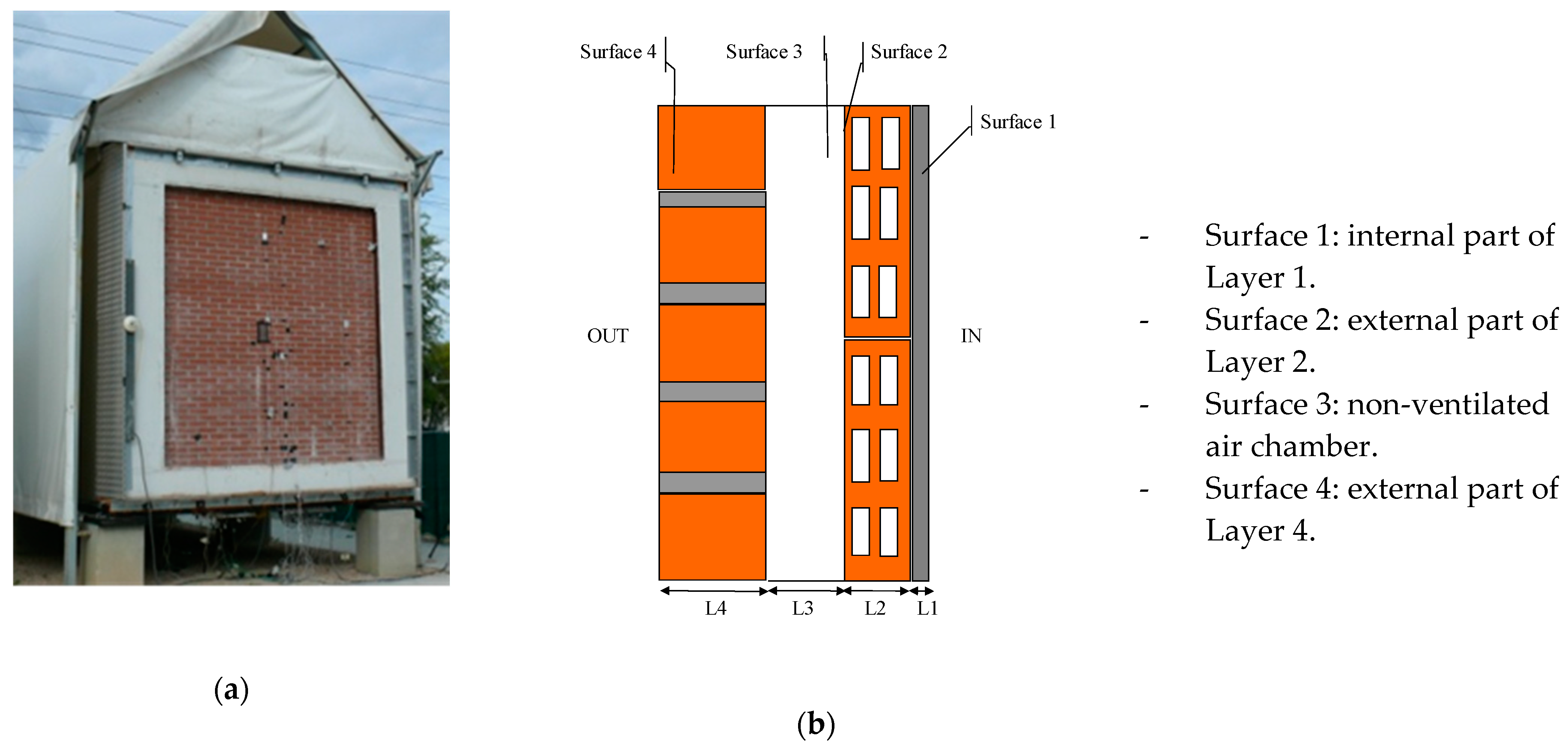
An OVF and an MLW were installed on the same double-leaf BW on the south wall of the same PASLINK test cell. The goal was to characterize and compare the thermal performance of both retrofit solutions and to quantify the potential for passive energy savings. The samples tested have external dimensions of 2.7 × 2.7 m, giving a sample area of 7.3 m².

Both passive solutions were installed on the south facade of the same PASLINK cell, on the same reference BW facade without insulation, in order to compare the improvements. Consequently, any differences in energy consumption and thermal performance between these solutions are exclusively attributed to their respective structures.

The decision to use either modular living systems or geotextile living wall systems depends on specific project requirements, preferences, and considerations. Modular systems offer advantages such as structured design, versatility, ease of installation, accessibility for maintenance, scalability, budget considerations, and customization options. Geotextile systems, on the other hand, offer a more organic appearance but require more manual labor for planting and maintenance.

In this study, the decision was made to assemble a modular vegetative facade. This decision was based on project objectives, aesthetic preferences, budget constraints, and maintenance considerations. The structured design, ease of installation, and adaptability of modular systems were particularly advantageous in meeting the specific goals and constraints of this project.

The passive system solutions assessed in this research consist of the following layers:

(a)

The base wall (BW) (see Figure 2) is constructed of the following surfaces: Layer 1: thick cement mortar (1.5 cm), Layer 2: double hollow brick (32 cm × 14 cm × 6.4 cm thick), Layer 3: non-ventilated air chamber (10 cm), and Layer 4: perforated brick (22.8 cm × 49 cm × 10.5 cm thick).

(b)

The OVF is installed on the outer layer of the BW (see Figure 3). Its component layers are installed from the inside to the outside: Layer 1–4: double-leaf base wall (BW), Layer 5: rock wool (5 cm), Layer 6: ventilated air chamber (5 cm), which contains a metallic substructure bearing anchored to the facade of the BW with screws, and Layer 7: ceramic panels (50 cm × 100 cm × 1.2 cm thick).

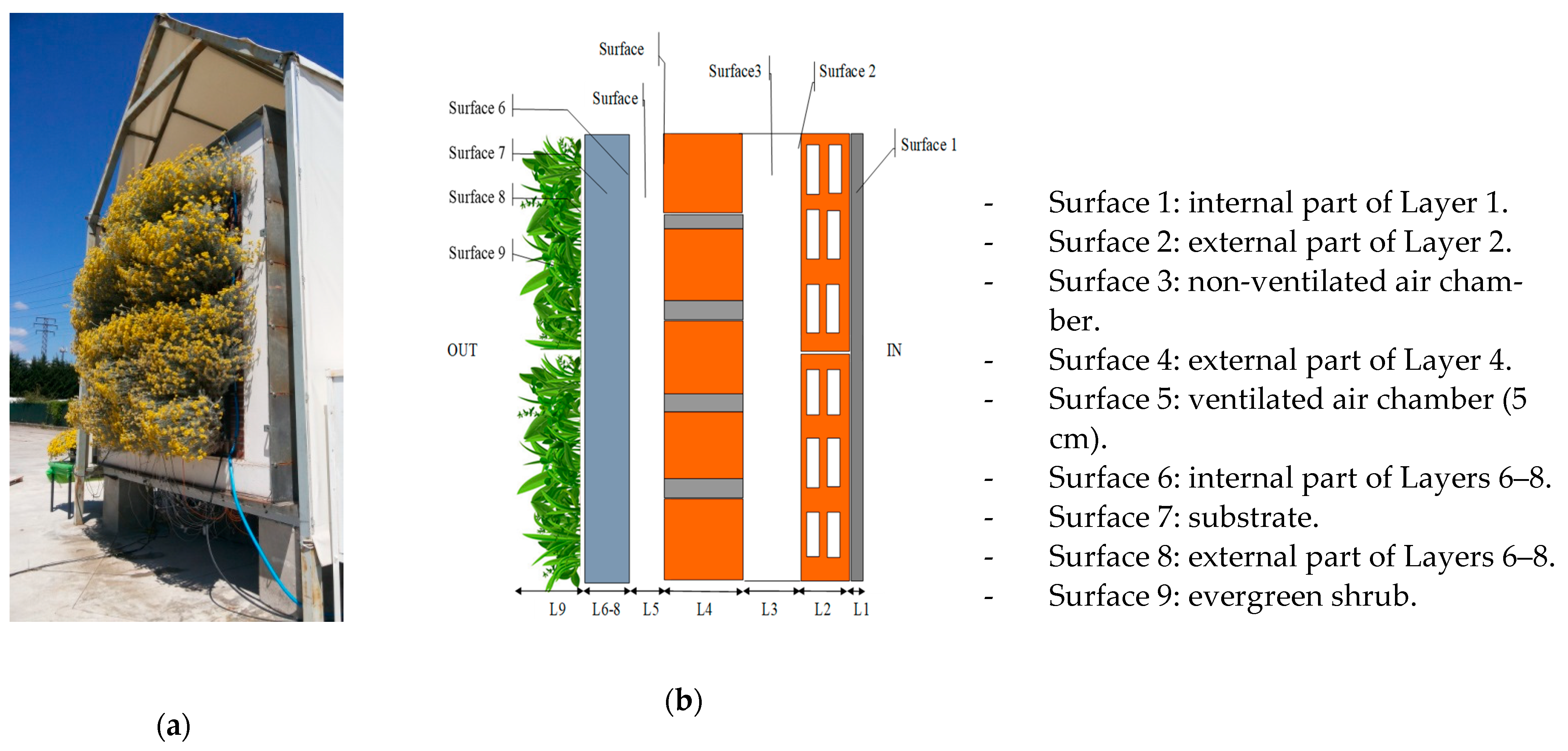
(c)

The chosen vertical greening system (VGS) is a modular living wall (MLW) (see Figure 4) made of recycled polyethylene modules measuring 600 × 400 × 80 mm. These square modules are filled with coconut fiber substrate. Each module has four micro-irrigation tubes at the top for watering and two drainage tubes at the bottom. The MLW receives approximately 2 L/m² of water per day during the summer, watering early in the morning (6 a.m.). In the fall, it receives approximately 1.5 L/m² per day. An evergreen shrub called Helichrysum italicum was chosen as the outer layer to ensure a uniform vegetative facade and to withstand cold winters.

The MLW is positioned on top of the double-leaf BW (Layers 1–4). From the inside to the outside, it is composed of the following layers: Layer 5: non-ventilated air chamber (5 cm), which houses a metal substructure based on stainless steel profiles fixed to the wall with metal screws. Layers 6–8: structure and module plus substrate (60 cm × 40 cm × 8 cm thick). Layer 9: vegetation layer with an evergreen shrub.

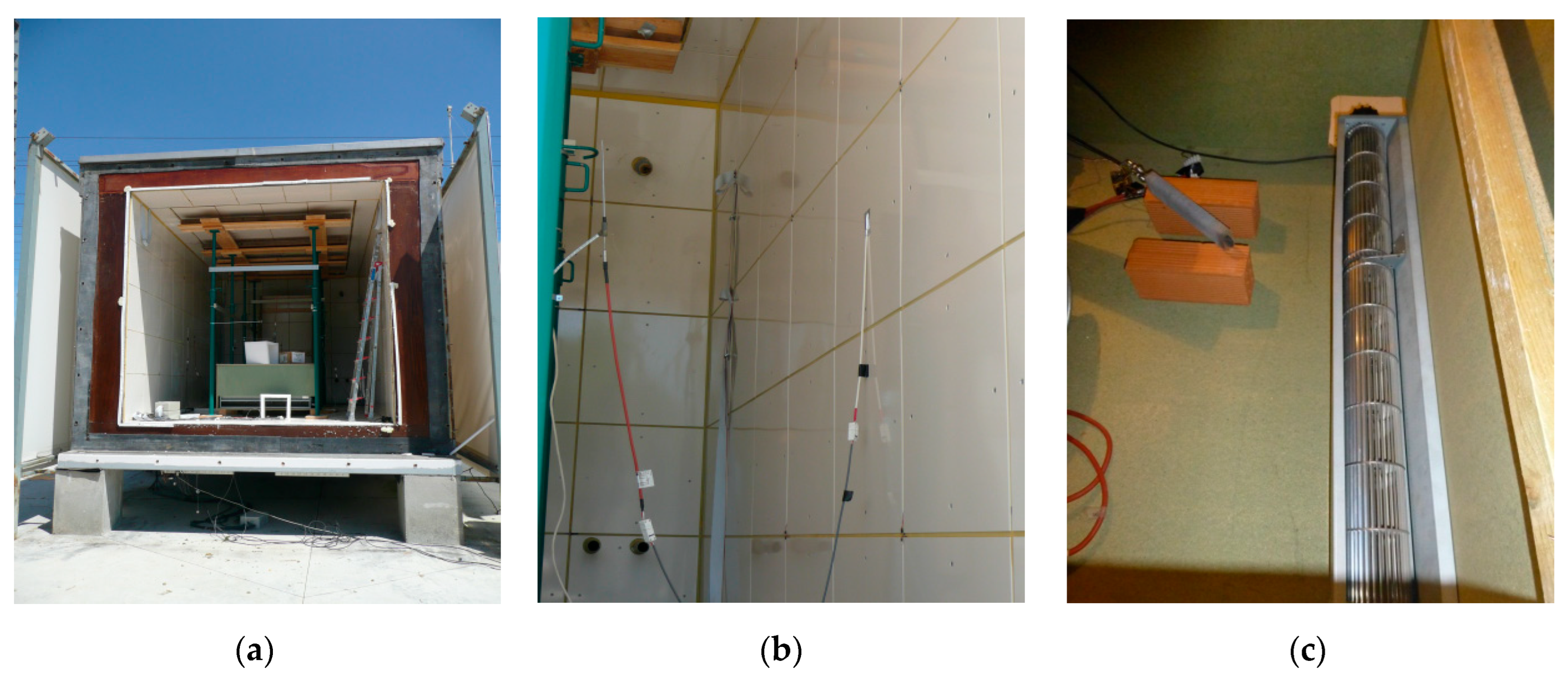
2.2. Data Acquisition and Sensors

This study shows the outcomes of three monitoring campaigns aimed at evaluating the advantages of passive building envelope solutions in terms of energy performance. The primary parameters studied include exterior surface temperatures with and without the passive system, solar radiation, outdoor air temperature, and heat fluxes through the different layers of the building.

There were three phases to the monitoring program described in this study. The first phase of the monitoring campaign described in this paper took place during the months of June and July 2012 (dataset A). During this time, the installation, transfer, and monitoring of the double-sided vertical BW were completed. Second, the installation and monitoring of the OVF was completed in August 2012 (dataset B). Finally, the installation of the MLW on the BW and its monitoring were completed in 2014 (dataset C).

Data period A includes the months of June and July. From January 2013 to December 2014, this study monitored a vegetated facade for two years. Despite covering both years, this article focuses on the 2014 summer dataset for two reasons.

First, in 2013, the monitored plants had limited growth, making them smaller and less effective. Therefore, the dataset from this year may not fully represent the dynamics of the vegetation facade. Second, focusing on a summer dataset allows for a meaningful comparison between three different facades under summer weather conditions. Emphasizing a specific time period with comparable meteorological conditions enhances the clarity and validity of comparative analyses, allowing for more focused and interpretable results.

The instrumentation and data acquisition monitoring of the PASLINK test cells were performed according to the guidelines provided in the PASLINK cell measurement and calibration manuals [47,48,49]. In addition, all necessary sensors such as temperature, heat flux, solar radiation, air temperature, and air velocity were installed according to the PASLINK manual specifications.

To evaluate the thermal performance of the two different construction systems, i.e., the OVF and MLW, installed on the same BW, the data presented in

Table 1. Instrumentation in the sample.

Number and Parameter per Layer	Instrument	Location in Each Layer	Range/Factor	Precision
One surface heat flux measurement	Almemo plates HFP-01	HF in z = 1.5 m middle	50 to 120 (W/m2)	±5%
Four surface temperatures per layer (*)	PT100 sensors class A 1/5 DIN	ST01 in z = 2.7 m middle	−20 to 60 °C	±0.1 °C
		ST02 in z = 1.5 m middle
		ST03 in z = 1.5 m east
		ST04 in z = 0 m middle
Four air temperatures in middle axis of air chamber (**)	PT100 sensors class A 1/5 DIN	ACT01 at 2.4 m height	−20 to 60 °C	±0.2 °C
		ACT02 at 1.8 m height
		ACT03 at 1.2 m height
		ACT04 at 0.6 m height
Four air velocities in the middle axis of the air chamber (**)	Hot Film Anemometer EE66-V	ACV01 at 2.4 m height	0 to 1 m/s	±0.1 m/s ±2% mV
		ACV02 at 1.8 m height
		ACV03 at 1.2 m height
		ACV04 at 0.6 m height
Electrical consumption		One in the interior	400 W	±0.5 W/s
Exterior air temperature	PT100 sensors class A 1/5 DIN	One in the exterior ATE01 protected against radiation and mechanically ventilated	−20 to 60 °C	±0.1 °C
Interior air temperature	PT100 sensors class A 1/5 DIN	One in the center of the test room ATI01 protected against radiation and mechanically ventilated	−20 to 60 °C	±0.1 °C
Pyranometer	Kipp&Zone CM11-P	One in the exterior layer in z = 2.7 m east	7 to 4000 W/m²	±3%

Note *: The average of the four surface temperature signals was considered the layer temperature. **: Air chamber layer in the case of the OVF is Layer 6 and Layer 5 for the MLW.

were collected at one-minute intervals and averaged every ten minutes.

The PASLINK test room is highly insulated and fully monitored, maintaining a constant temperature compared with the fluctuating outside temperature due to its advanced insulation and monitoring capabilities. The centrally located axial fan prevents temperature stratification within the chamber over time. The internal details of the test cell, including air and surface temperature sensors and the fan, are shown in Figure 5.

The calibration process incorporates factors such as edge effects, thermal bridging, and air infiltration as calibration considerations. Four temperature sensors per layer were used to measure the surface temperature across different layers of the sample. While the primary goal was to capture the core profile, an additional three sensors per layer were installed to investigate potential edge effects. These additional measurements helped to verify the one-dimensionality of the flow.

3. Methodology

The PASLINK procedure is used to obtain a physically interpreted model using statistical tools to identify the thermal system [49]. The initial model is a grey box RC concentrated parameter model that links a set of time-continuous ordinary differential equations to a dataset of measurements collected at discrete time points.

This paper presents the use of the data collected in the PASLINK test cell for the definition of a state-space model, or a so-called grey box model, based on an RC network for two vertical passive systems: the OVF and MLW. State-space models represent the different elements that make up the facade by resistances and capacitance modeling of building thermal dynamics as a linear time-invariant system. Grey box modeling is an iterative process, starting with a simpler model and gradually increasing the complexity until a good model fit is achieved. A multilayer envelope can be defined simply by 2 thermal resistances, a capacitance, and an internal node [50].

The LORD software package [51], developed during the PASLINK projects, allows for the modeling and identification of thermal systems with a special focus on building components. While a certain level of experience is required for its accurate application, the software uses the well-established lumped parameter modeling technique, representing the thermal system as an electrical analog RC network. Several enhancements, such as the stochastic treatment of data, have been implemented, resulting in improved results and a wider range of applications for the package.

The experimental setup of the two passive facades in the same BW and in the same PASLINK test cell allows for temperature and heat flux-controlled tests. To perform active measurements, it is necessary to apply an artificial thermal load to the PASLINK test cell. In order to obtain a reliable dataset for subsequent data analysis, an average temperature difference of approximately 20 °C between the inside and outside of the component being measured is required. The heating or cooling signals generated in the test chamber of the PASLINK test cell must not be related to the external temperature; otherwise, the data analysis technology will not be able to correctly characterize the thermal behavior of the analyzed component when analyzing the measured dynamic data. Therefore, the PRBS signal [52] (pseudo-random binary sequence, low-frequency routine with 60-min steps) was used as a heating or cooling signal during the test.

The PRBS sequence has a low-frequency pattern, which serves a dual purpose. Firstly, it enables the acquisition of datasets containing information about the low-frequency response of the components being tested. Secondly, as the heat input signal is completely uncorrelated with the external environmental conditions, it provides optimal conditions for parameter identification.

This sequence routine (ON/OFF), as mentioned above, lacks a correlation with other heat input streams (solar heat). It is designed to dynamically simulate the interior of the test cell by distributing the heat flux at different frequencies. These variations in the on and off times of the resistance thermometer range from 60-min to 12-h intervals.

In the experiments, PRBS sequences are used to obtain datasets containing the low-frequency response information on the device under test, completely decoupled from the external environmental conditions. This allows for parameters to be determined in optimal conditions. Throughout this study, the temperature of all layers as well as the ventilated air chambers and the heat flux of all layers of each of the building systems are compared.

To evaluate the thermal effect, the warm season of the year was taken into account. The thermal resistance of different layers of the building solutions was characterized. The thermal resistance depends on the thermal conductivity and the thickness of each layer and is an indicator of the resistance to heat flux through the layer.

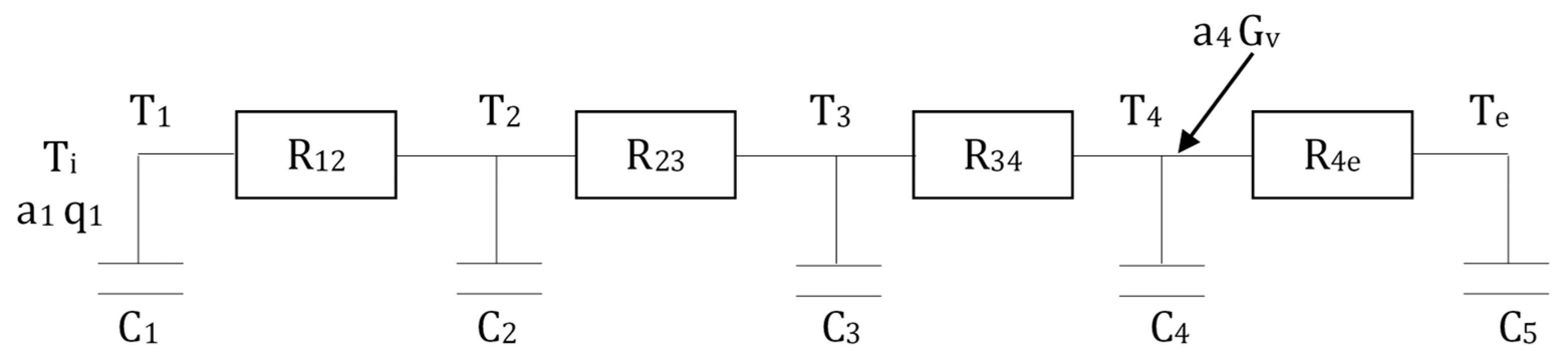
3.1. Thermal RC Network of the BW (Data Pool A)

The thermal behavior of the BW can be accurately replicated with the developed RC model. The model was created using the parameter modeling techniques outlined by the PASLINK network, specifically the parameter identification technique, which was implemented using an iterative process. After obtaining the RC model, it was transformed into a numerical model that facilitated the calculation of the BW for each time step. Subsequently, this numerical model was validated using data from all monitored layers under summer conditions. As a result, the RC network shown in Figure 6 represents the final model for the BW.

The stochastic differential equations representing the heat transfer process in Surface 1 are presented below. These equations take into account the heat input from the heater and solar radiation, as well as the capacitance and conductive heat flux within Surface 1. The remaining surfaces that make up the BW are treated similarly.

$$d{T}_1=\left(\frac{1}{C_1{·R}_{12}}\left(T_2-T_1\right)+\frac{a_1·q_1}{C_1}\right)dt$$

(1)

$$d{T}_2=\left(\frac{1}{C_2{·R}_{12}}\left(T_1-T_2\right)+\frac{1}{C_2{·R}_{23}}\left(T_3-T_2\right)\right)dt$$

(2)

$$d{T}_3=\left(\frac{1}{C_3{·R}_{23}}\left(T_2-T_3\right)+\frac{1}{C_3{·R}_{34}}\left(T_4-T_3\right)\right)dt$$

(3)

$$d{T}_4=\left(\frac{1}{C_4{·R}_{34}}\left(T_3-T_4\right)+\frac{1}{C_4{·R}_{4e}}\left(T_e-T_4\right)+\frac{a_4·G_v}{C_4}\right)dt$$

(4)

$$d{T}_e=\left(\frac{1}{C_5{·R}_{4e}}\left(T_4-T_e\right)\right)dt$$

(5)

The measured values are the surface layer temperatures T₁ to T₄, the external heat flux (q₁) on in Surface 1, the global vertical radiation (G_v), and the exterior air temperature (T_e). As a result, the wall thermal resistances (R₁₂, R₂₃, R₃₄, and R_4e) and capacitances (C₁, C₂, C₃, C₄, and C₅) can be calculated.

The variables q₁, G_v, and T_e are data for the model and are known for all time intervals since they are measured values. The aperture value (a₁) is equal to 1 for the measured heat fluxes, but (a₄) is not equal to 1, as just part of the incident radiation is absorbed by the outside surface of the BW, so it must be identified.

Using the input data for the time intervals, the LORD program (v3.2) was used to calculate the rest of the temperatures. Once the output variables were defined, the software calculated the values of the parameters of the system and used them until it succeeded in minimizing the objective function.

Therefore, grey box parameter models describe the heat transfer through the BW. A stochastic model is obtained as effects not described by the given deterministic model are added as noise. This case can be represented as follows:

$${V_N\left(\theta \right)=\frac{1}{N}\sum _{k=1}^N{‖{\epsilon }_k\left(\theta \right)‖}^2=\frac{1}{N}\sum _{k=1}^N{\left(\left(T_{Layer1,obs}-T_{Layer1,calc}\right)\right)}^2}_{.}$$

(6)

Following the same procedure (RC model) used in this section, the heat transfer parameters of the different surfaces that make up the base wall, i.e., from Layer 2 to Layer 3 and from Layer 3 to Layer 4, were calculated. In this way, the other parameters characterizing these components were quantified.

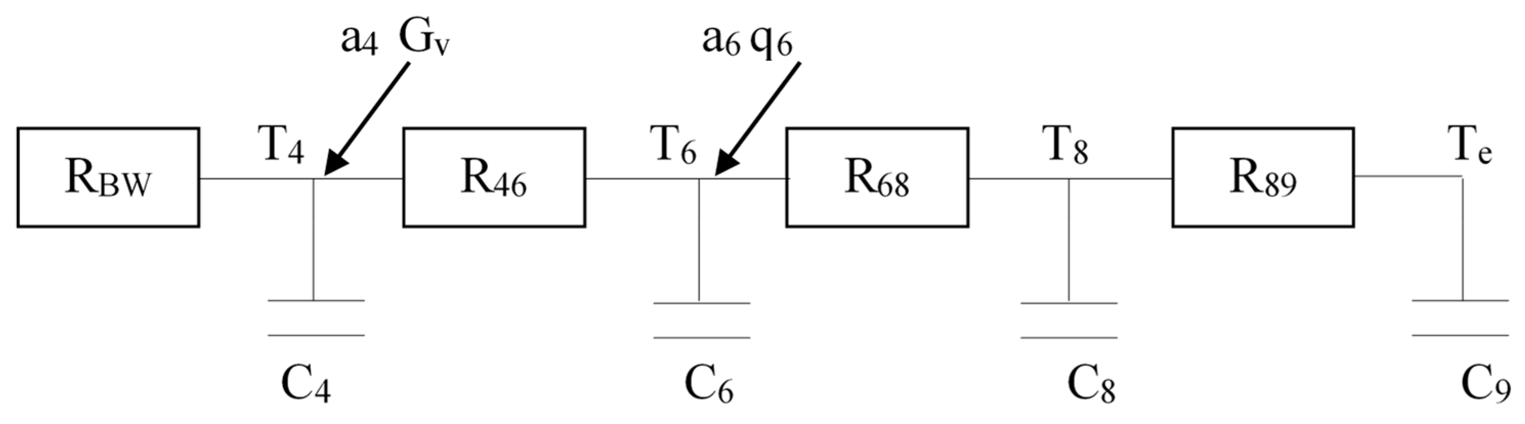
3.2. RC Network of the OVF (Data Pool B)

The heat transfer equations for the model shown in Figure 7 are given below:

$$d{T}_4=\left(\frac{1}{C_4{·R}_{45}}\left(T_5-T_4\right)+\frac{a_4·q_4}{C_4}\right)dt$$

(7)

$$d{T}_5=\left(\frac{1}{C_5{·R}_{45}}\left(T_4-T_5\right)+\frac{1}{C_5{·R}_{56}}\left(T_6-T_5\right)+\frac{a_5·G_v}{C_5}\right)dt$$

(8)

$$d{T}_6=\left(\frac{1}{C_6{·R}_{56}}\left(T_5-T_6\right)+\frac{1}{C_6{·R}_{68}}\left(T_8-T_6\right)\right)dt$$

(9)

$$d{T}_e=\left(\frac{1}{C_8{·R}_{68}}\left(T_6-T_e\right)\right)dt$$

(10)

The model was used assuming the following inputs: q₄ (for this case, HF04), T_e (ATE01), and G_v, while T₄ (temperature of Layer 4) was taken as output. These inputs and outputs were used in LORD software for different assumptions to achieve the identification of the parameters (all units of the equation are in (W/m²)).

Using the input data for time intervals k = 1, …, N, LORD software was used to calculate the remaining temperatures. Once the output variables were defined, the software calculated the values of the parameters in the system of equations in Equation (11) until it succeeded in minimizing the objective function. This case is represented as follows:

$${V_N\left(\theta \right)=\frac{1}{N}\sum _{k=1}^N{‖{\epsilon }_k\left(\theta \right)‖}^2=\frac{1}{N}\sum _{k=1}^N{\left(\left(T_{Layer4,obs}-T_{Layer4,calc}\right)\right)}^2}_{.}$$

(11)

The same procedure (RC model) used in this section was used to calculate the thermal characteristics of the other layers that make up the OVF.

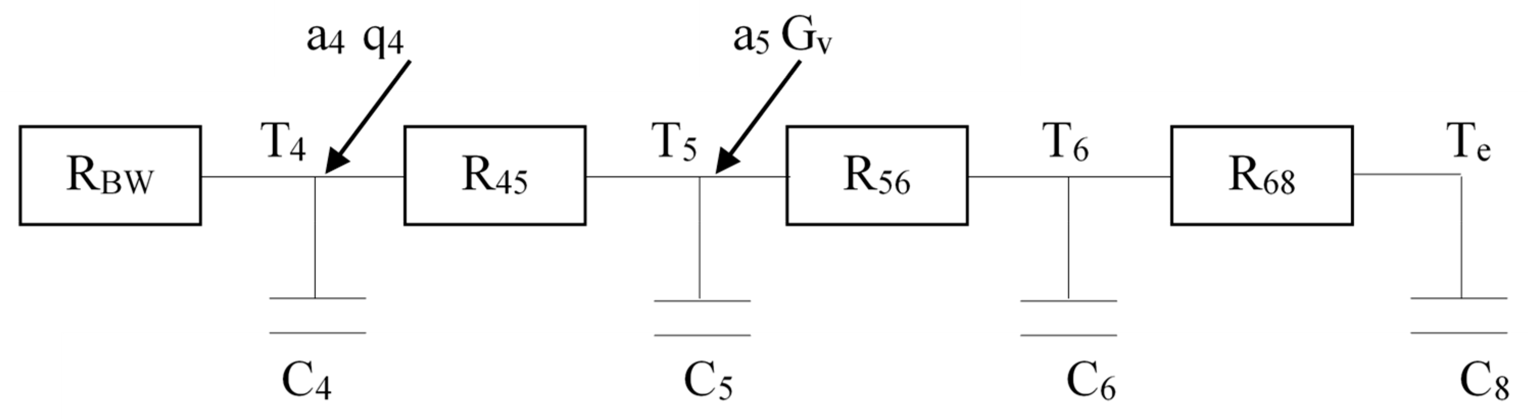
3.3. RC Network of the MLW (Data Pool C)

The PRBS sequences from 9 July to 17 July 2014 were used to calculate the thermal parameters of the MLW.

First, the equations governing the heat transfer process in the model shown in Figure 8 are presented.

$$d{T}_4=\left(\frac{1}{C_4{·R}_{46}}\left(T_6-T_4\right)+\frac{a_4·G_v}{C_4}\right)dt$$

(12)

$$d{T}_6=\left(\frac{1}{C_6{·R}_{46}}\left(T_4-T_6\right)+\frac{1}{C_6}·\left(T_8-T_6\right)+\frac{a_6·q_6}{C_6}\right)dt$$

(13)

$$d{T}_8=\left(\frac{1}{C_8{·R}_{68}}\left(T_6-T_8\right)+\frac{1}{C_8{·R}_{89}}\left(T_9-T_8\right)\right)dt$$

(14)

$$d{T}_e=\left(\frac{1}{C_9{·R}_{89}}\left(T_8-T_e\right)\right)dt$$

(15)

The model was used assuming the following inputs: q₆ (in this case HF06), T₉ = T_e = ATE01, and G_v, while T₄ (Layer 4 temperature) was taken as output. These inputs and outputs were used in LORD software for different assumptions to achieve the identification of the parameters.

The variables q₆, G_v, and T₉ are data for the model and are known for all time intervals, as they are measured values. The aperture value (a₆) is equal to 1 for the measured heat fluxes, but (a₄) is not equal to 1. It is necessary to identify the outer surface of the BW, which absorbs only a fraction of the incident radiation.

Using the input data for time intervals k = 1, …, N, LORD software was used to calculate the remaining temperatures. Once the output variables were defined, the software calculated the values of the parameters of the system of equations in Equation (16) until it minimized the objective function. This case is represented as follows:

$${V_N\left(\theta \right)=\frac{1}{N}\sum _{k=1}^N{‖{\epsilon }_k\left(\theta \right)‖}^2=\frac{1}{N}\sum _{k=1}^N{\left(\left(T_{Layer4,obs}-T_{Layer4,calc}\right)\right)}^2}_{.}$$

(16)

The same procedure (RC model) used in this section was used to calculate the thermal characteristics of the other layers that make up the MLW.

4. Results and Discussion

Firstly, the temperatures, heat fluxes, and climatic data collected in the PASLINK test cell with the three construction solutions for representative summer days are presented and discussed according to the insulation level and the absence or presence of vegetation. The thermal performance of the two systems and their cooling effect in the summer was studied using the RC model, which was validated with experimental results. Furthermore, the influence of the air chambers used in the two building solutions was evaluated, and the results were discussed regarding energy savings.

4.1. Temperature, Heat Flux, and Climate Profiles

4.1.1. BW Temperature, Heat Flux, and Climate Profiles (Data Pool A)

This section presents the data measured in the PASLINK test cell during nine representative summer days of the BW construction system. First, the average temperature data per layer are presented as well as the PRBS series carried out. Secondly, the indoor and outdoor air temperatures are presented, as well as the plot of the vertical solar radiation values and finally, the plot of the heat flux values through each of the layers comprising the BW of the selected period (22–30 of June).

The thermal pulses generated by the PRBS cycle cause an instantaneous reaction in both the internal environment of the PASLINK cell and the temperature of the first layer. As a result, these temperatures remain independent of the day/night cycle that affects the outer layers of the cell.

Figure 9 illustrates the sequence that the temperature of Layer 1 and the inner air follow. Conversely, the outermost layers experience temperature oscillations that closely resemble the day/night temperature changes that occur outside the cell, which are closely correlated with solar radiation. The fluctuation in the influx and outflux is observed throughout the day/night period, which gives the relationship between the heat fluxes.

During the sampled days, the average peak solar radiation was 500 W/m², and they were sunny days (except June 27 and 30). During hot summer days with intense radiation, the air temperature is lower than the last layer of the building wall (BW) due to the energy accumulated in the BW layers. The surface temperature of the facade increases significantly when exposed to solar radiation and then decreases when the radiation subsides.

The remarkable inertia of the wall at night plays a crucial role in maintaining the temperature of the outermost layer. This inertia prevents the temperature from dropping below the ambient temperature. For example, between 25 June and 28 June, both Layer 4 and Layer 3 consistently recorded temperatures above 40 °C, even though the ambient air temperature did not exceed 34 °C at its highest temperature. This phenomenon highlights the insulating effect of the wall, suggesting that its thermal mass retains heat and prevents rapid cooling during the night.

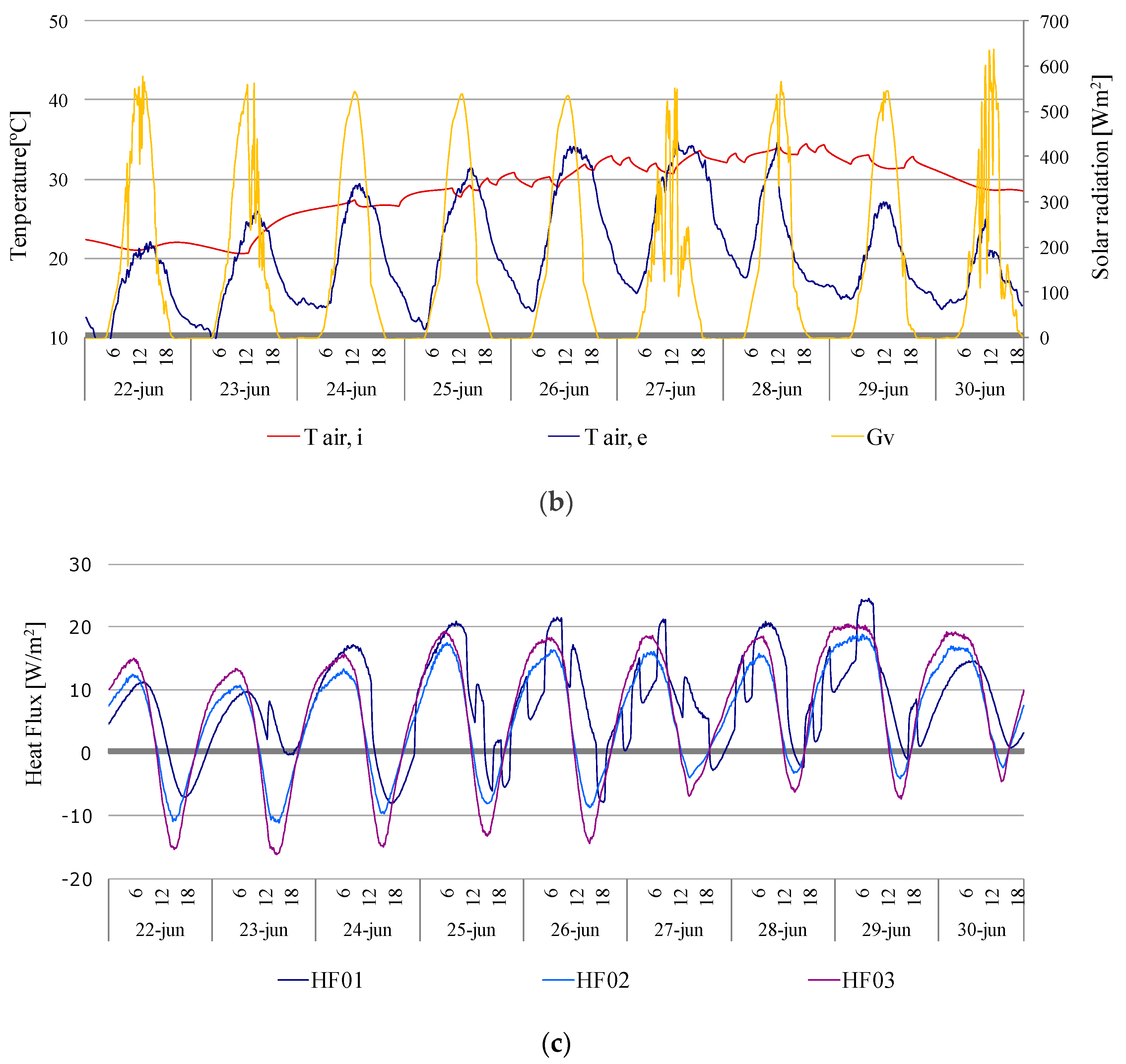
4.1.2. OVF Temperature, Heat Flux, and Climate Profiles (Data Pool B)

For the PRBS sequences carried out from 7 to 15 August 2012, a total of 9 days, as shown in Figure 9, were used to calculate the thermal parameters of the OVF. During this time frame, the climatic conditions experienced in Vitoria-Gasteiz, located in an oceanic climate zone, accurately reflected the prevailing weather patterns of this urban area. Typically, the temperature reaches its highest point during the afternoon hours, usually around 30 °C. Occasionally, it can rise even higher, reaching 40 °C. In addition, on days with clear skies, the vertical solar radiation measures approximately 620 W/m².

Figure 10 illustrates the thermal inertia of each component and shows distinct characteristics. It can be seen that the indoor air temperature reacts quickly when the heating is activated. On the other hand, the internal surface of the OVF, and, in particular, the temperature of the exterior layers, shows a much higher level of stability.

Observing the previous figures, in layer number one, a rapid response of temperature is observed to the power cycles carried out during the sampling sequence. The layers that make up the base wall (Layer 1 to Layer 4) present the same trend but with a lower temperature per layer, around 0.2 °C less per layer.

During the sunny hours, there is a 25% reduction in heat transfer into the room compared with the BW. In addition, the losses during the night can be considered insignificant. With respect to the north facade, the OVF shows a slightly better performance during the day and only minor differences during the night.

On the other hand, throughout the data sequence, the high global vertical solar radiation (700 W/m²) produces an increase in the outside temperature as well as that of the outer layers (Layers 5–8), reaching maximum temperatures at noon 12.00 h. The maximum temperature was reached on 10 August, reaching 52 °C in the outer layer, while the inside of the test cell was 35 °C. This strong solar incidence is also reflected in the HF06 and HF07 exterior flux meters, while the indoor flush meters follow the resistance thermometer sequence.

It was verified that the incoming heat flux on the ventilated facade reaches values −40 W/m² in the central hours of the day, during periods without solar radiation. Especially during the night, this value becomes positive and approaches values of 5 W/m².

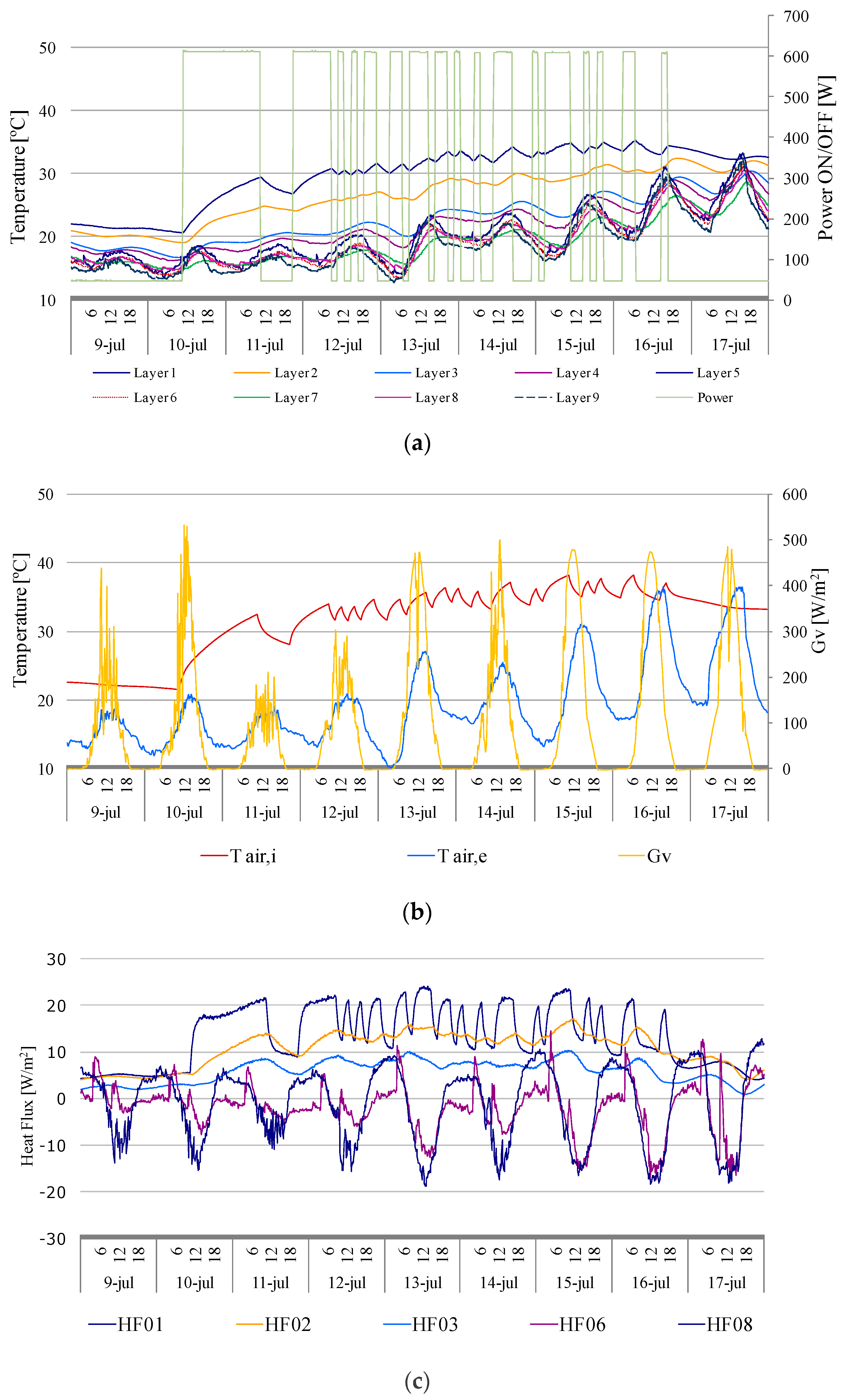
4.1.3. MLW Temperature, Heat Flux, and Climate Profiles (Data Pool C)

The implementation of a VGS on the exterior surface has a significant impact on preventing solar radiation from reaching the wall. This in turn ensures that the surface temperature does not increase, as shown in Figure 10. The comparison of the exterior and interior surface temperatures with the outdoor air temperature shows that the vegetation surface temperature can be up to 10 °C cooler than the outdoor environment during the hottest hours of the day. However, the maximum temperature difference between the outside air temperature (T_air,e in Figure 10b) and the last layer of the MLW (Layer 9 in Figure 10a) at night is only 2 °C, depending on the outside conditions. The outdoor temperature is closely related to solar radiation, which peaks at 36 °C. When the radiation drops to peak values of 200 W/m², the outdoor temperature drops to about 20 °C. In both cases, the LW temperature remains stable and below the outdoor air temperature.

As mentioned earlier, it is evident that the temperature in the outermost layer of the BW is higher than that in the outermost layer of the MLW. The highest temperature observed within a 24-h period is greater in the BW (ranging from 40 to 43 °C) compared with the MLW (ranging from 31 to 34 °C) when the outdoor air temperature and peak solar radiation are at the same level (31–34 °C and 500 W/m², respectively). This discrepancy is particularly observed between the dates of June 26 (Figure 8) and July 17 (Figure 11). The data obtained from this study are considered comparable due to the implementation of two different construction solutions within a PASLINK test cell, where all test parameters are meticulously controlled and accurately measured both internally and externally.

The MLW and BW were compared at an outdoor air temperature of 31–36 °C, which showed that the MLW maintained temperatures below 32 °C while the brick facade reached 40 °C. This indicates that the temperature of the MLW is lower than the outdoor air temperature during the daytime. The cooling effect of the GW is most noticeable during peak heat hours, and the outermost surface temperature remains lower than the outside air temperature. This temperature reduction is likely due to a combination of factors, including evapotranspiration, solar shading, and additional thermal resistances provided by the substrate and air layer of the vegetated facade.

The temperature of the air in the space between the vegetation and the BW is a critical factor to consider. In July, the average temperature of the air in this space (see Layers 5 and 6) is 5 °C lower than the ambient air temperature. This temperature difference results in a reduction in the amount of energy required to maintain a cool indoor air temperature during the summer months. In addition, the air in this cavity can serve as a source of fresh air to cool the building facade. In essence, the air cavity created behind the green facade acts as an additional layer of thermal insulation.

4.2. Thermal Characterization

4.2.1. Measurement of the Base Wall’s Thermal Characteristics

The results of the identification of the parameters for the different construction elements that make up the BW can be seen in

Table 2. Results of the RC model of the BW for the different layers that compose it.

Layer	R (°C m2/W)	C (kJ/°C m2)	Residual
Layers 1–2 Cement mortar 1.5 cm+ Hollow double brick 6.4 cm	0.26	153.74	0.18
Layer 3 Non-ventilated air chamber 10 cm	0.37	0.00	0.19
Layer 4 Facing brick 10.5 cm	0.12	65.40	0.18
∑ Layers 1–4	0.75	219.14

. The first surface that makes up the BW, composed of cement mortar and hollow double brick, has a thermal resistance of 0.26 (°C m²)/W. The value of the second surface (non-ventilated air chamber) corresponds to a thermal resistance of 0.37 (°C m²)/W. Finally, the surface composed of facing bricks has one-third of the thermal resistance capacity of the other components.

The aperture parameter a₄ (0.34) represents the value of the effective absorptivity of the vertical global solar radiation in the external surface layer of the facing brick.

Validation was completed by fitting the data sequence and by checking the residuals. Errors in the sensors or any other type of non-linearity, such as temperature dependence, can occur during the sequence analyzed, and these errors are observed in the residuals, the unadjusted part of the sequence. In the above model identification, it is observed that the RMS error of the residuals is 0.18; therefore, the error committed is less than the precision error of the signals. The results obtained with the LORD program can be considered correct.

4.2.2. Measurement of Thermal Characteristics OVF

The results of the identification of the parameters for the different construction elements that make up the OVF are shown in

Table 3. Results of the RC model of the ventilated facade for the different layers.

Layer	R (°C m2/W)	C (kJ/°C m2)	Residual
Layers 1–4 (BW)	0.75	245
Layer 5 Rock wool 5 cm	1.59	235	0.65
Layer 6 Ventilated air chamber 5 cm	0.11	0
Layer 7 Ceramic plate 1.2 cm	0.026	35	0.94
∑ Layers 1–7 (OVF)	2.47	470

.

As can be seen in Table 3, the first element after the BW has a very high thermal resistance of 1.59 (°C m²)/W. This construction element, comprising 5 cm of rock wool, acts as the insulation in the OVF and provides the exact insulation required by the BW in a hypothetical facade renovation. The next surface, the ventilated air chamber, has a thermal resistance of 0.11 (°C m²)/W, and finally, the ceramic plates have a low thermal resistance of 0.026 (°C m²)/W.

As a result of the values of the parameters identified in the OVF, it can be seen how the sum of the elements that make up the OVF on the base wall gives it additional thermal insulating properties.

Comparing the data obtained from the OVF with the data obtained from the BW before the renovation, the main difference with the integration of this element lies in the improved insulating capacity of the ventilated facade. This improvement is due to the addition of 5 cm of rock wool and the air chamber, which contributes an additional thermal resistance of 1.70 (°C m²)/W. This confirms that the OVF makes a positive contribution to thermal insulation. When this parameter was measured in the OVF, an a₅ value of 0.21 was recorded. Comparing the value of this construction solution with the value of the double BW of 0.34, an increase in cooling capacity of 60% is obtained. These results show that the implementation of the OVF is beneficial for indoor comfort. The positive impact on the thermal balance of the facade during the summer season highlights the effectiveness of the OVF in contributing to a more favorable and comfortable indoor environment.

4.2.3. Measurement of Thermal Characteristics MLW

Table 4. Results of the RC model of the modular living wall for the different layers.

Layer	R (°C m2/W)	C (kJ/°C m2)	Residual
Layers 1–4 (BW)	0.75	205.56	0.94
Layer 5 Ventilated air chamber 5 cm	0.10	0
Layers 6–8 MLW module + substrate 8 cm	0.23	96.12	0.26
Layer 9 Vegetation 50 cm	0.14	12.03	0.64
∑ Layer 19 (MLW)	1.22	313.71

below shows the thermal parameters of the different layers that make up the MLW. The ventilated air chamber provides a thermal resistance of 0.10 (°C m²)/W, the MLW provides 0.23 (°C m²)/W, and finally, the vegetation provides 0.14 (°C m²)/W. Therefore, the positive effect on the insulation of the constructive solution is observed thanks to the MLW since the incorporation of this constructive element improves the insulation of the initial BW.

Analyzing the results observed during the summer season, it is clear that the focus of comfort is on the cooling of the external surface of the facade due to the maximum radiation and external temperatures. By reducing the effective absorptivity coefficient of the wall, the temperature of the greened facade is reduced, resulting in a favorable result for MLWs. This makes them a viable option for passive temperature reduction.

In parallel with the measurements of the thermal parameters, the absorptivity (a₄) of the MLW was analyzed, resulting in a value of 0.11 (-), which represents a reduction of 68% compared with the initial situation of the BW. This characteristic could be one of the main reasons for the cooling of the facade.

The MLW is effective in reducing the need for air conditioning in the summer season. The continuous evapotranspiration of the plants leads to a reduction in the temperature of the outer layer of the facade. Therefore, if the goal is to renovate a building envelope to reduce heat loss, it is recommended that a layer of insulation be added to the BW prior to installation of the system.

Therefore, if an enclosure needs to be renovated to minimize heat loss, it is recommended that the BW be insulated before installing the vegetated system.

In the MLW, the thermal characteristics show improvements. In this case, it went from a thermal transmittance of the BW of 0.75 W/(m² °C) and an effective absorptivity of 0.34 to a thermal transmittance of 1.22 W/(m² °C) (increase in insulating capacity of 30%) and an effective absorptivity of 0.10 (increase in the cooling capacity of 68%).

5. Conclusions

The thermal refurbishment consisted of constructing a modular living wall without any insulating elements other than the vegetation module itself, which includes the substrate and the plants. The aim was different from the aims mentioned in the introduction, which was to “evaluate the thermal performance of two passive facade systems”, an MLW and an OVF, in comparison to a conventional building solution BW for building rehabilitation. The results obtained with this retrofit solution are significantly lower than those of the OVF solution, reaching values of 0.37 (°C m²/W). For the ventilated facade, it should also be noted that by adding 5 cm of rock wool to the base wall (1.59 °C m²/W), the modular living wall would achieve a quantitative increase in insulation capacity.

Increasing thermal comfort means reducing the influence of external temperature extremes on the internal temperature of the building and thus reducing the energy required to maintain the internal temperature, either via cooling or heating. The results obtained for the effective absorptivity of the different solutions analyzed (base wall: 0.34 (-), open-ventilated facade: 0.21 (-), and modular living wall: 0.11 (-)) show that both open-ventilated and vegetated facades can be used as passive cooling strategies. In the case of the open ventilated facade, the percentage reduction is 60%, while for the modular living wall; the percentages are higher, reaching 68% of the initial situation.

To optimize the benefits of passive building envelopes, the selection of appropriate sustainable building materials is critical. The use of these design solutions could reduce the temperature of the buildings during the hot season, improving occupant comfort and reducing energy demand.

References

1. Onyszkiewicz, J.; Sadowski, K. Proposals for the revitalization of prefabricated building facades in terms of the principles of sustainable development and social participation. J. Build. Eng. 2022, 46, 103713. [Google Scholar] [CrossRef]
2. Janjua, S.Y.; Sarker, P.K.; Biswas, W.K. Sustainability implications of service life on residential buildings—An application of life cycle sustainability assessment framework. Environ. Sustain. Indic. 2021, 10, 100109. [Google Scholar] [CrossRef]
3. Blanco, J.M.; Buruaga, A.; Cuadrado, J.; Zapico, A. Assessment of the influence of façade location and orientation in indoor environment of double-skin building envelopes with perforated metal sheets. Build. Environ. 2019, 163, 106325. [Google Scholar] [CrossRef]
4. Jankovic, A.; Siddiqui, M.S.; Goia, F. Laboratory testbed and methods for flexible characterization of thermal and fluid dynamic behaviour of double skin facades. Build. Environ. 2022, 210, 108700. [Google Scholar] [CrossRef]
5. Sotelo-Salas, C.; Pozo, C.E.; Esparza-López, C.J. Thermal assessment of spray evaporative cooling in opaque double skin facade for cooling load reduction in hot arid climate. J. Build. Eng. 2021, 38, 102156. [Google Scholar] [CrossRef]
6. Girma, G.M.; Tariku, F. Experimental investigation of cavity air gap depth for enhanced thermal performance of ventilated rain-screen walls. Build. Environ. 2021, 194, 107710. [Google Scholar] [CrossRef]
7. Maciel, A.C.F.; Carvalho, M.T. Operational energy of opaque ventilated façades in Brazil. J. Build. Eng. 2019, 25, 100775. [Google Scholar] [CrossRef]
8. Sanjuan, C.; Suárez, M.J.; González, M.; Pistono, J.; Blanco, E. Energy performance of an open-joint ventilated façade compared with a conventional sealed cavity façade. Sol. Energy 2011, 85, 1851–1863. [Google Scholar] [CrossRef]
9. Preet, S.; Mathur, J.; Mathur, S. Influence of geometric design parameters of double skin façade on its thermal and fluid dynamics behavior: A comprehensive review. Sol. Energy 2022, 236, 249–279. [Google Scholar] [CrossRef]
10. Pastori, S.; Mereu, R.; Mazzucchelli, E.S.; Passoni, S.; Dotelli, G. Energy Performance Evaluation of a Ventilated Façade System through CFD Modeling and Comparison with International Standards. Energies 2021, 14, 193. [Google Scholar] [CrossRef]
11. Zhang, W.; Gong, T.; Ma, S.; Zhou, J.; Zhao, Y. Study on the Influence of Mounting Dimensions of PV Array on Module Temperature in Open-Joint Photovoltaic Ventilated Double-Skin Façades. Sustainability 2021, 13, 5027. [Google Scholar] [CrossRef]
12. Wang, Y.; Chen, Y.; Li, C. Airflow modeling based on zonal method for natural ventilated double skin façade with Venetian blinds. Energy Build. 2019, 191, 211–223. [Google Scholar] [CrossRef]
13. Pujadas-Gispert, E.; Alsailani, M.; van Dijk, K.C.A.; Rozema, A.D.K.; ten Hoope, J.P.; Korevaar, C.C.; Moonen, S.P.G. Design, construction, and thermal performance evaluation of an innovative bio-based ventilated façade. Front. Archit. Res. 2020, 9, 681–696. [Google Scholar] [CrossRef]
14. Pizzatto, S.M.D.S.; Pizzatto, F.O.; Angioletto, E.; Arcaro, S.; Junca, E.; Klegues Montedo, O.R. Thermal evaluation of the use of porous ceramic plates on ventilated façades—Part II: Thermal behavior. Int. J. Appl. Ceram. Technol. 2021, 18, 1734–1742. [Google Scholar] [CrossRef]
15. Nizovtsev, M.I.; Letushko, V.N.; Yu Borodulin, V.; Sterlyagov, A.N. Experimental studies of the thermo and humidity state of a new building facade insulation system based on panels with ventilated channels. Energy Build. 2020, 206, 109607. [Google Scholar] [CrossRef]
16. Ling, H.; Wang, L.; Chen, C.; Chen, H. Numerical investigations of optimal phase change material incorporated into ventilated walls. Energy 2019, 172, 1187–1197. [Google Scholar] [CrossRef]
17. Benzarti, S.; Chaabane, M.; Mhiri, H.; Bournot, P. Performance improvement of a naturally ventilated building integrated photovoltaic system using twisted baffle inserts. J. Build. Eng. 2022, 53, 104553. [Google Scholar] [CrossRef]
18. Agathokleous, R.A.; Kalogirou, S.A. Status, barriers and perspectives of building integrated photovoltaic systems. Energy 2020, 191, 116471. [Google Scholar] [CrossRef]
19. Cuce, E.; Cuce, P.M. Optimised performance of a thermally resistive PV glazing technology: An experimental validation. Energy Rep. 2019, 5, 1185–1195. [Google Scholar] [CrossRef]
20. Gagliano, A.; Aneli, S. Analysis of the energy performance of an Opaque Ventilated Façade under winter and summer weather conditions. Sol. Energy 2020, 205, 531–544. [Google Scholar] [CrossRef]
21. Ciampi, M.; Leccese, F.; Tuoni, G. Ventilated facades energy performance in summer cooling of buildings. Sol. Energy 2003, 75, 491–502. [Google Scholar] [CrossRef]
22. De Masi, R.F.; Festa, V.; Ruggiero, S.; Vanoli, G.P. Environmentally friendly opaque ventilated façade for wall retrofit: One year of in-field analysis in Mediterranean climate. Sol. Energy 2021, 228, 495–515. [Google Scholar] [CrossRef]
23. Rahiminejad, M.; Khovalyg, D. Numerical and experimental study of the dynamic thermal resistance of ventilated air-spaces behind passive and active façades. Build. Environ. 2022, 225, 109616. [Google Scholar] [CrossRef]
24. Baldinelli, G. A methodology for experimental evaluations of low-e barriers thermal properties: Field tests and comparison with theoretical models. Build. Environ. 2010, 45, 1016–1024. [Google Scholar] [CrossRef]
25. Gagliano, A.; Nocera, F.; Aneli, S. Thermodynamic analysis of ventilated façades under different wind conditions in summer period. Energy Build. 2016, 122, 131–139. [Google Scholar] [CrossRef]
26. Susorova, I. 5—Green facades and living walls: Vertical vegetation as a construction material to reduce building cooling loads. In Eco-Efficient Materials for Mitigating Building Cooling Needs; Pacheco-Torgal, F., Labrincha, J.A., Cabeza, L.F., Granqvist, C., Eds.; Woodhead Publishing: Oxford, UK, 2015; pp. 127–153. [Google Scholar]
27. Jim, C.Y. Thermal performance of climber greenwalls: Effects of solar irradiance and orientation. Appl. Energy 2015, 154, 631–643. [Google Scholar] [CrossRef]
28. Susca, T. Green roofs to reduce building energy use? A review on key structural factors of green roofs and their effects on urban climate. Build. Environ. 2019, 162, 106273. [Google Scholar] [CrossRef]
29. Djedjig, R.; Bozonnet, E.; Belarbi, R. Experimental study of the urban microclimate mitigation potential of green roofs and green walls in street canyons. Int. J. Low-Carbon. Technol. 2015, 10, 34–44. [Google Scholar] [CrossRef]
30. Hop, M.E.C.M.; Hiemstra, J.A. Contribution of green roofs and green walls to ecosystem services of urban green. Acta Hortic. 2013, 475–480. [Google Scholar] [CrossRef]
31. Mayrand, F.; Clergeau, P. Green Roofs and Green Walls for Biodiversity Conservation: A Contribution to Urban Connectivity? Sustainability 2018, 10, 985. [Google Scholar] [CrossRef]
32. Azkorra, Z.; Pérez, G.; Coma, J.; Cabeza, L.F.; Bures, S.; Álvaro, J.E.; Erkoreka, A.; Urrestarazu, M. Evaluation of green walls as a passive acoustic insulation system for buildings. Appl. Acoust. 2015, 89, 46–56. [Google Scholar] [CrossRef]
33. Francis, R.A.; Lorimer, J. Urban reconciliation ecology: The potential of living roofs and walls. J. Environ. Manag. 2011, 92, 1429–1437. [Google Scholar] [CrossRef] [PubMed]
34. Taleghani, M. Outdoor thermal comfort by different heat mitigation strategies- A review. Renew. Sustain. Energy Rev. 2018, 81, 2011–2018. [Google Scholar] [CrossRef]
35. Iaria, J.; Susca, T. Analytic Hierarchy Processes (AHP) evaluation of green roof- and green wall- based UHI mitigation strategies via ENVI-met simulations. Urban. Clim. 2022, 46, 101293. [Google Scholar] [CrossRef]
36. He, B. Towards the next generation of green building for urban heat island mitigation: Zero UHI impact building. Sustain. Cities Soc. 2019, 50, 101647. [Google Scholar] [CrossRef]
37. Pérez, G.; Coma, J.; Martorell, I.; Cabeza, L.F. Vertical Greenery Systems (VGS) for energy saving in buildings: A review. Renew. Sustain. Energy Rev. 2014, 39, 139–165. [Google Scholar] [CrossRef]
38. Yungstein, Y.; Helman, D. Cooling, CO2 reduction, and energy-saving benefits of a green-living wall in an actual workplace. Build. Environ. 2023, 236, 110220. [Google Scholar] [CrossRef]
39. He, Q.; Tapia, F.; Reith, A. Quantifying the influence of nature-based solutions on building cooling and heating energy demand: A climate specific review. Renew. Sustain. Energy Rev. 2023, 186, 113660. [Google Scholar] [CrossRef]
40. Azkorra-Larrinaga, Z.; Erkoreka-González, A.; Flores-Abascal, I.; Pérez-Iribarren, E.; Romero-Antón, N. Defining the cooling and heating solar efficiency of a building component skin: Application to a modular living wall. Appl. Therm. Eng. 2022, 210, 118403. [Google Scholar] [CrossRef]
41. Oquendo-Di Cosola, V.; Olivieri, F.; Ruiz-García, L. A systematic review of the impact of green walls on urban comfort: Temperature reduction and noise attenuation. Renew. Sustain. Energy Rev. 2022, 162, 112463. [Google Scholar] [CrossRef]
42. Coma, J.; Pérez, G.; de Gracia, A.; Burés, S.; Urrestarazu, M.; Cabeza, L.F. Vertical greenery systems for energy savings in buildings: A comparative study between green walls and green facades. Build. Environ. 2017, 111, 228–237. [Google Scholar] [CrossRef]
43. Djedjig, R.; Belarbi, R.; Bozonnet, E. Experimental study of green walls impacts on buildings in summer and winter under an oceanic climate. Energy Build. 2017, 150, 403–411. [Google Scholar] [CrossRef]
44. Medl, A.; Florineth, F.; Kikuta, S.B.; Mayr, S. Irrigation of ‘Green walls’ is necessary to avoid drought stress of grass vegetation (Phleum pratense L.). Ecol. Eng. 2018, 113, 21–26. [Google Scholar] [CrossRef]
45. Cheng, C.Y.; Cheung, K.K.S.; Chu, L.M. Thermal performance of a vegetated cladding system on facade walls. Build. Environ. 2010, 45, 1779–1787. [Google Scholar] [CrossRef]
46. Chen, M.; Chen, L.; Cheng, J.; Yu, J. Identifying interlinkages between urbanization and Sustainable Development Goals. Geogr. Sustain. 2022, 3, 339–346. [Google Scholar] [CrossRef]
47. van der Linden, G.P.; van Dijk, H.A.L.; Lock, A.J.; van der Graaf, F. COMPASS Installation Guide HFS Tiles for the PASSYS Test Cells; JOULE II–COMPASS: Brussels, Belgium, 1995. [Google Scholar]
48. Maldonado, E. PASSYS Operations Manual; FEUP. CEC DGXII: Brussels, Belgium, 1993. [Google Scholar]
49. Saxhof, B. PASLINK Calibration Manual. In A Revision of the PASSYS Calibration Manual; Stanzel, B., Ed.; ITW University of Stuttgart: Stuttgart, Germany, 1995. [Google Scholar]
50. Ramallo-González, A.P.; Eames, M.E.; Coley, D.A. Lumped parameter models for building thermal modelling: An analytic approach to simplifying complex multi-layered constructions. Energy Build. 2013, 60, 174–184. [Google Scholar] [CrossRef]
51. Gutschker, O. Parameter identification with the software package LORD. Build. Environ. 2008, 43, 163–169. [Google Scholar] [CrossRef]
52. Letherman, K.M.; Palin, C.J.; Park, P.M. The measurement of dynamic thermal response in rooms using pseudo-random binary sequences. Build. Environ. 1982, 17, 11–16. [Google Scholar] [CrossRef]
Figure 1. (a) Details of the exterior of the PASLINK test cell: west-facing facade. (b) Interior of the test cell without a sample: south-facing facade.
Sustainability 15 16737 g001
Figure 2. (a) The detailed appearance of the studied BW. (b) The detailed structure of the BW in the test setup in the PASLINK experimental cell.
Sustainability 15 16737 g002
Figure 3. (a) The detailed appearance of the studied OVF. (b) The detailed structure of the OVF in the test setup in the PASLINK experimental cell.
Sustainability 15 16737 g003
Figure 4. (a) The detailed appearance of the studied MLW. (b) The detailed structure of the MLW in the test setup in the PASLINK experimental cell.
Sustainability 15 16737 g004
Figure 5. (a) Front view of the ILARGI test cell: the south wall where the test sample is positioned. (b) Air temperature and internal surface temperature sensors used in the tests. (c) A green fireproof box housed the electric heater and axial fan to prevent temperature stratification within the test cell.
Sustainability 15 16737 g005
Figure 6. RC network used to determine the thermal characteristics of the BW.
Sustainability 15 16737 g006
Figure 7. RC network used to determine the thermal characteristics of the OVF.
Sustainability 15 16737 g007
Figure 8. RC network used to determine the thermal characteristics of the MLW.
Sustainability 15 16737 g008
Figure 9. (a) PRBS runs at the BW with thermal evolution at different layers. (b): Evolution of the temperature of the indoor air, the temperature of the outdoor air, and the vertical global radiation during the PRBS run. (c) Thermal flux sensor evolution in the different layers of the sample along the PRBS run (June).
Sustainability 15 16737 g009aSustainability 15 16737 g009b
Figure 10. (a) PRBS runs at the BW with thermal evolution at different layers. (b) Evolution of the temperature of the indoor air, the temperature of the outdoor air, and the vertical global radiation during the PRBS run. (c) Thermal flux sensor evolution in the different layers of the sample along the PRBS run (August).
Sustainability 15 16737 g010
Figure 11. (a) PRBS runs at the BW with thermal evolution at different layers. (b) Evolution of the temperature of the indoor air, the temperature of the outdoor air, and the vertical global radiation during the PRBS run. (c) Thermal flux sensor evolution in the different layers of the sample along the PRBS run (July).
Sustainability 15 16737 g011