Abstract
The renovation of public lighting installations by replacing the traditional systems with LED technologies and introducing smart lighting control systems is a policy widely adopted to contain energy consumption and expenditure. Additionally, the long-term monitoring of the depreciation of the new lighting systems is a crucial issue. The aim of this study is to report the results of in-field measurements of new LED lighting systems in the city of Turin (Italy). A method was defined to assess: (i) energy performance (through data from the remote-control system); (ii) photometric performance (through in-field measurement campaigns); and (iii) depreciation of the photometric performance over a period of approximately 5 years. Results demonstrated that the new LED systems allow us to achieve an average energy saving of 51% compared to the ex-ante condition, improving the photometric performances and compiling the standard requirements by lowering the over-illumination levels. Moreover, the measured depreciation of the LED systems over time was compared with the predicted depreciation, estimated based on the calculation method proposed in Standards BS 5489-1:2020 and ISO/CIE TS 22012:2019. The results obtained showed that the measured depreciation of the photometric performance was closer to the predicted depreciation trend according to BS 5489-1:2020 (variations between 0% and 4%), while greater variations (between 17% and 23%) emerged considering the ISO/CIE TS 22012:2019.
1. Introduction
Public lighting is an essential service for cities and has a primary role in ensuring visibility and the safety of users during night-time. It represents a public service that influences citizens’ well-being in several aspects, such as their perception of safety [1], crime prevention [2], social interactions, etc. Moreover, outdoor lighting systems allow us to define urban night-time image [3,4], improving the appearance of cities and landscape contexts and enhancing the cultural asset [5]. Providing high-quality outdoor lighting is therefore essential to ensure a good quality of life for citizens and urban users. Nevertheless, public lighting systems also have a relevant impact in terms of energy consumption and light pollution, representing one of the most significant expenses in the municipal administrations budget, primarily due to energy and maintenance costs. According to [6], the annual energy consumption for road lighting in Europe was approximately 35 TWh, representing 1.3% of the energy consumption of electricity. For municipalities, outdoor urban lighting installations significantly affect up to 80% of the total use of electricity, and public street lighting can account for up to 40–60% of a city’s budget energy expenditure [7,8]. Moreover, previous research demonstrated that in Europe, most of the lighting installations were designed some decades ago and are therefore obsolete and inefficient [9]. According to the data, about two-thirds of the lighting installations in the EU are from the 1960s, 1970s and 1980s, and in 2012, only 10% of new public streetlights were LED-based [10].
In this frame, the introduction of more sustainable and efficient systems represents an opportunity to improve energy efficiency and reduce costs and CO2 emissions, moving toward the concept of Smart Cities [11]. Many international organizations, such as the European Union (EU) and the International Energy Agency (IEA), have undertaken policies to encourage the adoption of energy savings strategies and efficiency policies also related to public lighting [12,13]. Lighting Europe’s Strategy Roadmap 2025 [14] suggests the adoption of new profitable approaches, such as “LEDification” and the introduction of intelligent lighting systems. The implementation of outdoor lighting is also recognized as a vector directly impacting the Sustainable Development Goals (SDGs) defined by the United Nations, contributing to solving some existing issues related to SDG targets [15]. Furthermore, the adoption of more sustainable solutions in outdoor lighting systems is promoted within EU financing projects (see as an example the research and development project “REPLICATE—Renaissance of Places with Innovative Citizenship And Technologies” funded by the EU’s Horizon 2020 Research and Innovation program and aimed at deploying energy efficiency, mobility and ICT solutions while also considering the smart public lighting sector [16]).
Thanks to the important technological innovation that occurred in the field of lighting during the last decades, nowadays, the adoption of new technologies, i.e., the replacement of obsolete luminaires with new LEDs (light-emitting diodes) and/or the introduction of smart lighting control systems, allows us to significantly reduce the operating costs for both energy consumption and maintenance [17]. LED technology is currently considered a satisfactory solution thanks to its low energy consumption, high luminous efficiency, long life, reduced investment and maintenance costs, and lower environmental impact [18,19]. As a consequence, during recent years, many public authorities have undertaken a renovation process concerning their public lighting systems. The most frequently adopted measures involve the replacement of obsolete luminaires with old light sources with more efficient lighting technologies (e.g., light-emitting diode (LED)) and/or the introduction of smart lighting control systems. It is demonstrated that the simple adoption of energy-efficient LED lighting can provide potential energy savings between 50 and 70% compared to the old technologies, with considerable benefit to tight city budgets and a good return on investment [20,21,22,23,24]. Moreover, in terms of environmental sustainability, a potential saving of more than 1400 million tons of CO2 [7] can be achieved, and the investments cannot be only profitable and sustainable but also improve lighting quality [25]. Besides the luminaires’ substitution, the implementation of advanced control systems can further increase the economic and energy sustainability of public lighting systems. Pilot projects demonstrated that the integration of smart lighting control systems enables a significant reduction in energy consumption compared to traditional control systems [26,27], particularly when employing full adaptive installations (FAIs) [28,29]. In the literature, several studies have reported results about the effectiveness of interventions based on the renovation of the public lighting systems with more efficient ones, along with the introduction of dynamic lighting management (see a review in [7]). In general, results underlined that the refurbishment with LED technologies and the introduction of a control system allow for better results in terms of reduction of CO2 emissions and energy savings, with significant positive impacts from an economic, social, and environmental point of view [9].
The reported framework demonstrated the potential effectiveness of lighting optimization interventions, in terms of both energy efficiency and reduction of costs for municipalities, along with improving visual comfort and citizens’ safety. In this frame, the assessment of the performances of new installations and the comparison between traditional lighting systems and newly installed ones (in terms of photometric performance, energy, and economic savings) were conducted by simulation methods and/or in-field measurements [30,31,32,33,34]. In particular, the energy (and consequently economic) savings were assessed by monitoring in-field the energy consumption data and/or through the estimation of energy performance indicators. Instead, simulation methods were mainly used to assess the photometric performances of a lighting system, since simulation tools are nowadays considered affordable and promising techniques in the field of lighting optimization [35].
Besides comparing the performances of traditional and newly installed lighting systems, the assessment and monitoring of the photometric and energy performances of the new lighting systems over time is a crucial issue. Indeed, throughout the useful life of any lighting installation, the light emission, and so the light available for the visual task, progressively decreases. The rate of reduction depends on different factors, such as the type of lamps, luminaires, environment, and operation conditions, and length of time they are used [36]. During the design phase of a lighting system, light loss (or depreciation) has to be considered through the application of a maintenance factor to luminaire photometric data, to ensure that at the end of the design life of a specific lighting installation, the minimum required lighting level is still maintained. In other words, the maintenance factor reflects how the light output decreases over time, considering several different aspects such as the luminous flux depreciation, the environmental parameters, the maintenance, the cleaning intervals, etc. Within this frame, the PD ISO/CIE TS 22012:2019 “Light and lighting. Maintenance factor determination. Way of working” [37] is currently the main reference for the determination of the maintenance factor, also considering the increasing use of new technologies with different technical characteristics, such as LED. Furthermore, other national standard references such as the BS 5489-1:2020 [38] report the calculation method for determining the overall maintenance factor, as well as examples and typical values. Generally, during the design phase of a lighting system, the maintenance factor value is determined based on parameters and reference values provided by manufacturers and standards, and it is implemented in the simulation phase to size the light installation so it fulfills the standard requirements over its entire lifetime. However, lighting simulation is still challenging because of the complexity of reflecting the actual conditions of an environment over time [35]. In the literature, studies on the photometric performances of lighting installations over time focused only on forecast estimates, while there are no studies reporting long-term monitoring based on measured data. Therefore, in this paper, a field measurement campaign was set up to monitor the long-term performance of new LED lighting systems, in order to assess the performances over time and to compare the actual depreciation of the systems to the one estimated based on the standard values.
Main Goals of the Paper
The main issues that emerged from the outlined reference framework are the following:
- The implementation of public lighting systems with more efficient ones is currently promoted and supported by funding policies;
- In the literature, some studies focused on the assessments of performances due to the retrofit of lighting systems (in terms of photometric performance, energy, and economic savings) [16,20,22,24,27,28,29,31,33,34] and on a comparison with the previous system [17,21,23,25,26,30,32]. While the energy performances were assessed by data measured through in-field monitoring, photometric performances were mainly evaluated using simulation tools [30,31,32,33,34];
- Also, the monitoring of the photometric and energy performances of the new lighting systems over time is a crucial issue, and current studies are focused only on forecast estimates;
- The design of new lighting installations is based on maintenance factors defined according to standard reference values, but there are no studies that report monitoring the depreciation of the actual performances of current LED lighting systems based on field measurements.
Based on these considerations, the aim of the study presented in this paper is to report the results of in-field measurements aimed at assessing and monitoring the photometric and energy performances of new LED lighting systems, after the implementation of a retrofit project. A selection of roads and pedestrian areas included in the lighting renovation program of the city of Turin (Italy) were chosen as a case study. Through regular monitoring, both energy performances (data acquired from the remote-control system) and photometric performances (data from in-field measuring campaigns) were assessed. In particular, the study addressed the following main objectives:
- To compare the energy performance of the previous traditional lighting system (ex-ante installation) with the new LED lighting systems (ex-post installation), in order to evaluate the energy saving;
- To compare the photometric performance of ex-ante and ex-post lighting systems and to monitor the performance of the new systems over a period of about 5 years (i.e., the duration of the monitoring campaign);
- To assess the depreciation of the photometric performance of the ex-post installations over the period of the monitoring campaign and to compare it with the predicted depreciation of the photometric performance, estimated based on the maintenance factor calculation method proposed by the standards.
In the following sections, the case study, the methodology adopted for the assessment and measurements of both lighting performance and energy performance, and the results obtained, as well as the comparison between predicted and measured depreciation of the lighting performance, are presented.
2. Case Study
The city of Turin (Italy) in 2015 implemented the “Torino a LED” project, which involved a program to renovate the public lighting system. The project consisted of the substitution of 55,000 luminaires of the public lighting systems, equipped with traditional high-pressure sodium or metal-halide technologies, with LED luminaires. Areas with different characteristics were involved in the replacement: traffic roads, pedestrian paths, squares, and parks. The primary goal of the project was energy saving, estimated at 20,000 MWh/year, corresponding to a reduction of 3.5 tons/year of CO2 emissions. Moreover, additional energy savings were expected thanks to the adoption of a control system designed to dim the light in steps during the night. The project was therefore qualified to obtain Energy Efficiency Certificates. In addition to energy saving, the project aims to ensure compliance with safety and visual comfort lighting performance requirements (as specified by technical standards), to increase the utilance of the lighting installations, to prevent obtrusive light, and to mitigate light pollution. The replacement of the luminaires was based on the outcomes of a comprehensive project that involved lighting simulations, in agreement with the specifications of the Urban Traffic Plan [39] and the Municipal Illumination Plan [40] and in accordance with both national and international technical regulations [41,42].
Within the “Torino a LED” project, in this study, a sample of significant motorized roads and pedestrian areas where the previous traditional lighting systems (ex-ante installations) were replaced with new LED lighting systems (ex-post installations) was considered. In particular, 12 traffic roads and 8 pedestrian areas, representative of the total types of renovated installations, were analyzed (Figure 1).
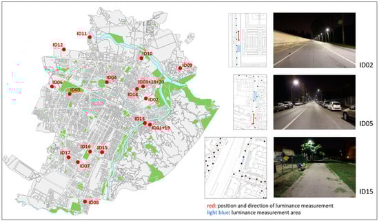
Figure 1.
On the left: plan view of the city of Turin (Italy) with indication of the locations of the area considered in the sample (ID 01 to ID 20). On the right: examples of the areas considered with indication of the individual lighting fixtures: ID 02—motorized traffic road; ID 05—motorized traffic road; ID 15—pedestrian area.
The considered motorized traffic roads (ID01 to ID12) were characterized by conventional paving made of asphalt. The roads were single or multiple carriageways, with at least one or two lanes for each direction. The ex-ante stock of installed luminaires consisted of traditional lighting sources, i.e., high-pressure sodium lamps (HPS), compact high-intensity discharge lamps (CDM) and metal-halide gas discharge lamps (HMI). The project of the ex-post installations involved the substitution of the ex-ante lighting system with LED technologies equipped with asymmetric street optics. Regarding the luminaires’ features, the luminaire installed power was reduced from 70–250 W (142 W on average) to 28.5–125 W (73 W on average), equal to an average reduction of 48%. Moreover, the project allowed us to increment the luminaire luminous efficacy from 49–83 Lm/W (66 Lm/W on average) in the ex-ante condition to 105–117 Lm/W (112 Lm/W on average) in the ex-post installation, equal to an average increase of 70%.
Concerning the pedestrian areas, the considered sample included paths located in park areas, footpaths, and a cycle path. Different luminaire typologies were installed. Park areas (ID13 to ID17) were equipped with pole-top floodlights with direct symmetrical light distribution, while the footpaths (ID19 and ID20) and the cycle path (ID18) were illuminated by the street lighting system described above. For what concern the park areas, the traditional light sources, consisting of compact high intensity discharge lamps (CDM) and mercury vapor lamps (HQL), were replaced with LEDs luminaires which maintained the direct symmetrical light distribution. The luminaire installed power was reduced from 100–250 W (155 W on average) to 43–53 W (49 W on average), equal to an average reduction of 68%. The luminaire luminous efficacy was incremented from 28–72 Lm/W (51.2 Lm/W on average) in the ex-ante condition to 81–92 Lm/W (87.6 Lm/W on average) in the ex-post installation, equal to an average increase of 71%.
Lamps of both motorized traffic roads and pedestrian areas in the ex-ante condition had a correlated color temperature (CCT) between 2000 and 3300 K and a color rendering index (CRI) between 20 and 89. The ex-post LED sources had a correlated color temperature (CCT) of 4000 K and CRI above 70. Moreover, LED chips from two different manufacturers (hereinafter LED01 and LED02) were installed in the luminaires of the sample considered in this study. Furthermore, the same LED chip was used in luminaires with different optics.
Data concerning the road geometry, arrangement of the lighting system, lighting class, lamp typology, installed power, luminous flux, and luminaire luminous efficacy of both ex-ante and ex-post installations of the analyzed motorized traffic roads and pedestrian areas are reported, respectively, in Table 1 and Table 2.

Table 1.
Abacus of the installed ex-ante and ex-post lighting systems in the analyzed motorized traffic roads.
Table 2.
Abacus of the installed ex-ante and ex-post lighting systems in the analyzed pedestrian areas.
Considering the control system of the lighting installations, both the ex-ante and ex-post lighting systems were switched on and off through a centralized remote-control system (switch-on threshold equal to 30 lx and astronomical clock reserve). The ex-ante lighting system was kept at full power throughout the whole night, while for the ex-post installation, a control system was adopted to dim the light in two stages during the night-time: from 12:00 a.m. to 01:00 a.m., the power is reduced by 10% (90% of nominal luminous flux), and from 01:00 a.m. to 06:00 a.m., the power is reduced by 30% (70% of nominal luminous flux). The average switch-on hours of the ex-post installation (4113 h average per year) spread throughout the 12 months are reported in Figure 2.
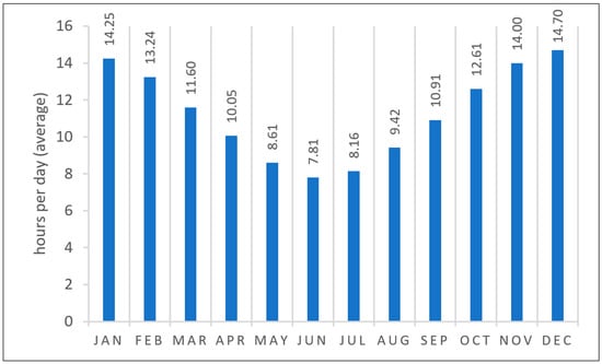
Figure 2.
Ex-post installation’s average daily switch-on hours for each month.
3. Methods
Considering the case study described above, a method was defined to assess and compare the photometric and energy performances of the ex-ante and ex-post installations and to monitor the performances of the ex-post systems over a period of approximately 5 years. The method was based on the acquisition of data through in-situ measurement campaigns and on the further elaboration of the same. In particular, the adopted method included different phases: (i) assessment of the energy performance (ex-ante and ex-post systems); (ii) assessment of the photometric performance (ex-ante and ex-post systems); and (iii) assessment of the depreciation of the photometric performance (ex-post system). A flowchart illustrating the methodological approach is reported in Figure 3, and further details about the method phases are reported in the following subsections.
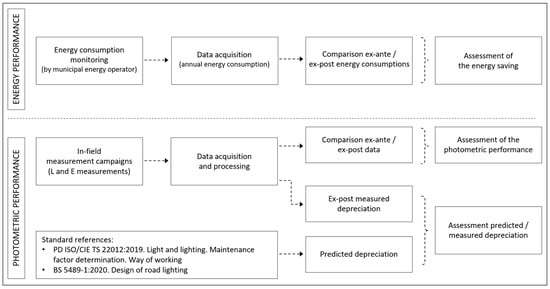
Figure 3.
Description of the methodological approach [37,38].
3.1. Assessment of the Energy Performance
The energy performance and, consequently, the energy consumption, of a lighting system are influenced by several factors. Key factors include the luminous efficacy of the lamps, the optical efficiency of the luminaires, and the energy losses associated with ballasts. Additionally, the efficacy in exploiting the emitted luminous flux, often determined by lighting design choices, is another significant factor. Finally, the type and features of the lighting control system, responsible for managing the on/off switching and light dimming, also have a direct impact on the annual energy consumption.
Within this study, the energy performances of both ex-ante and ex-post installations during the monitoring period were assessed. Data on the annual energy consumption of the switchboards connected to the sample areas were provided by the municipal energy operator. In particular, as regards the ex-ante condition, the annual energy consumption data provided by the municipal energy operator were calculated as the product of the installed power and the annual operational hours. Instead, as concerns the ex-post condition, the measured annual energy consumption data were provided. Based on these data, the ex-ante and ex-post energy consumptions of the considered switchboards were compared in order to assess the energy saving achieved through the retrofit of the lighting system. Moreover, the energy consumption trends over the 5 years of monitoring the new LED installations were evaluated.
3.2. Assessment of the Photometric Performance
Measurement campaigns were conducted in the field to verify the lighting conditions with both the ex-ante and the ex-post LED lighting systems. One measurement campaign was carried out to assess the lighting performance of the ex-ante lighting systems. After the LED retrofit (ex-post), five measurement campaigns were carried out in a time span of approximately 5 years, with a frequency of one measurement campaign about every year (C1–C5). The monitoring campaign started after the renovation of all lighting installations was completed and therefore the first measurement campaign (C1) was carried out with a variable delay compared to the switch-on of the initial LED luminaires. Furthermore, each year, the duration of the measurement campaign (i.e., the time required to perform the measurements for all the selected lighting installations) was also variable, due to different types of contingencies (e.g., weather conditions, availability of the municipal police, etc.) The lighting performance of both ex-ante and ex-post installations for each analyzed road and pedestrian area was assessed through in-situ photometric measurements. The measurement campaigns were based on illuminance and luminance data acquisition, in accordance with technical standards EN 13201 part 3 and part 4 [43,44].
Luminance measurements of the road surface were conducted for motorized traffic roads, while horizontal illuminance was measured for pedestrian and cycle areas. The installations were assessed at full power to verify compliance with standard requirements, considering the lighting class defined in the design phase [45]. For the luminance acquisition in motorized traffic roads, a TechnoTeam “LMK Mobile” ILMD (Image Luminance Measuring Device) (based on a Canon EOS digital camera) with a measurement uncertainty of 4.7% was used to assess the luminance distribution of the framed carriageway, represented as a luminance image. In this study, the static measurement method was adopted as described by EN 13201-4 [44] and CIE TR 194 [46]. The luminance image was captured with the observer positioned in the center of each traffic lane, 60 m away from the measuring area of the carriageway. The analysis of the luminance images followed a three-step process, as shown in Figure 4 and described as follows:
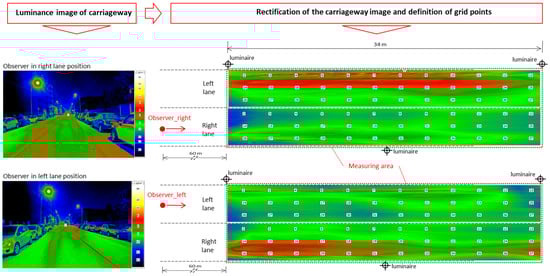
Figure 4.
Example of luminance image analysis for a two-lane carriageway motorized traffic road.
- Step (1): Luminance image acquisition of the relevant area of the carriageway;
- Step (2): Rectification of the luminance image and definition of the measuring grid;
- Step (3): Luminance data analysis (average value, overall and longitudinal uniformity).
In particular, in this study, the photometric performance assessment of roads with two lanes was based on the mean value of average luminances, referred to the entire carriageway and measured in each observer position at the center of the lane. This mean value of luminance was considered for data analysis, as described in Section 4 “Results”.
The static measurement system was preferred with respect to a dynamic one [47] since with the former it can be easier to control repeatability and reliability over time. The observer position with respect to the measured area (distance, camera height) was controlled in each measurement campaign by means of repeated distance measurements of specific reference points (i.e., a lighting pole in the measured area) and employing a photographic survey (i.e., horizontal road traffic signs as markers). As a consequence of the static method, the measurements of road luminance were always carried out without traffic, stopping necessarily the traffic on all lanes.
For pedestrian areas, horizontal illuminance was measured by means of a Minolta T-10M luxmeter with a measurement uncertainty of 2%, considering grid points at ground level.
Both luminance and illuminance measurements were taken in the 5 years of the study during the autumn and winter seasons. The measurement campaigns were conducted during night-time between September and February.
Throughout the measurement campaign, further information was acquired and recorded: the characteristics of the lighting system and its maintenance over time, the meteorological conditions and visibility, the asphalt condition (dry/wet) and its maintenance over time, and the presence of parasite lighting with respect to the relevant area.
The data obtained through the measurement campaigns were further investigated to evaluate the differences between ex-ante and ex-post photometric conditions, as well as the compliance of the new lighting systems with the standard requirements over the 5 years of analysis.
3.3. Assessment of the Depreciation of the Photometric Performance
The data measured during the 5 measurement campaigns (C1–C5) with the LED ex-post installations were also used to assess the depreciation of the photometric performance over time (approximately 5 years, i.e., the period between the luminaires’ substitution and the end of the monitoring period). The depreciation trends obtained from the measured data were then compared with the depreciation, estimated based on the calculation method proposed in the literature [37,38]. The final goal was to evaluate the consistency between actual and predicted trends.
The depreciation of the light output over time is defined as the ratio of the illuminance produced by the lighting system after a certain period to the illuminance produced by the system when new and is expressed by the maintenance factor (Equation (1)). Therefore, the maintenance factor trend reflects the light loss (or depreciation of the light output) of a given installation over time.
where:
- fM = maintenance factor
- Em = maintained illuminance
- Ein = initial illuminance
In this study, the depreciation of the light output of the considered sample installations was assessed using the data measured to assess the lighting performances of the installations, that is: (i) the road luminance for motorized traffic roads and (ii) the horizontal illuminance on the pavement for pedestrian areas. The maintenance factor f′M was therefore calculated as the ratio of luminance (or illuminance) referred to the lighting system at a given time (C1–C5) to the luminance (or illuminance) when the system was new (C0), as reported in the Equation (2).
where:
- f′M(L) = maintenance factor (photometric performance depreciation) calculated as luminance ratio
- f′M(E) = maintenance factor (photometric performance depreciation) calculated as illuminance ratio
- LCn = luminance measured at a given time (Cn)
- LC0 = luminance measured when the lighting system was new (C0)
- ECn = illuminance measured at a given time (Cn)
- EC0 = illuminance measured when the lighting system was new (C0)
The predicted depreciation of the same lighting systems was calculated assuming the standard maintenance factor calculation method. In particular, the PD ISO/CIE TS 22012:2019 [37] was assumed as a reference for the maintenance factor determination method, since it is currently considered as the latest best practice guidance. As reported in [37], the predicted maintenance factor (fM), is determined using the formula:
where:
fM = fLF · fS · fLM · fSM
- fLF = luminous flux factor—expresses the depreciation of the luminous flux over time due to the ageing of the light source or luminaire during regular operation. This is defined as the ratio of depreciated luminous flux to the initial luminous flux [37]. In general, for LED-based luminaires, the fLF shall be determined based on the light source or luminaire replacement interval and shall be provided by manufacturers. Methods and conditions for measuring the lumen maintenance of LEDs are provided by the IES (Illuminating Engineering Society of North America) LM-80-08 “Approved method for measuring lumen maintenance of LED light sources” [48] and IES TM-21-11 “Projecting long term lumen maintenance of LED light sources” [49]. fS = survival factor—expresses the probability of the light source and/or luminaire to continue to operate at a given time. This factor shall be based on the type of operational regime [37]. In this study, the fS was set equal to 1, since according to the operational regime adopted by the municipal operator, light sources are replaced directly in case of breakage.
- fLM = luminaire maintenance factor—expresses the relative output of the luminaire due to dirt deposited on light sources, optical components or other components influencing the luminaire output [37]. In particular, for outdoor luminaires, the determination of fLM shall be based on the combination of luminaire design (IP classification), environmental pollution category, and cleaning interval. References to fLM typical values are reported in different standards. In this study, two main references were assumed to determine the fLM: (i) PD ISO/CIE TS 22012:2019—Annex C.2 “Outdoor luminaires. Examples of outdoor luminaire maintenance factors fLM” [37] and (ii) BS 5489-1:2020 Annex C1 “Typical luminaire maintenance factors” [38].
Table 3.
Table from ISO/CIE TS 22012:2019—Annex C.2 “Outdoor luminaires. Examples of outdoor luminaire maintenance factors fLM” [37].
Table 4.
Table from BS 5489-1:2020 Annex C1 “Typical luminaire maintenance factors” [38].
- fSM = surface maintenance factor—considers the depreciation of surface reflection [37]. For outdoor lighting, except for tunnels and underpasses, the fSM is set to 1.00.
To compare actual and estimated depreciation trends, the overall lighting installation sample was divided into three subsets: (i) motorized and traffic roads with luminaires equipped with LED01, (ii) pedestrian areas (park areas) with luminaires equipped with LED02, and (iii) pedestrian areas (footpaths and cycling area) with luminaires equipped with LED01. The analysis was conducted separately for the three subsets since the measured photometric quantities and the characteristics of the LEDs, in terms of lumen maintenance, were different. For each subset, a regression analysis was applied to derive an overall measured depreciation trend to be compared to the estimated one.
4. Results
In this section, the results of the energy and lighting performance monitoring campaign of the sample of motorized traffic roads and pedestrian areas are reported.
4.1. Energy Performance
To assess the energy performances, the installed power, and the annual energy consumption data (expressed in kWh) of the switchboards, which included the areas of the sample, were provided by the municipal energy operator. Table 5 reports the installed power values of the considered switchboards for each year. Moreover, the calculated ex-ante and measured ex-post energy consumptions in the 5 years of monitoring were assessed (considering in both cases the total amount of energy consumption of the considered switchboards). Figure 5 shows the comparison between ex-ante and ex-post annual energy consumption data.
Table 5.
Installed power of the considered switchboards.
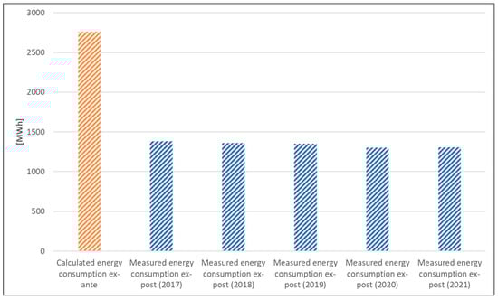
Figure 5.
Calculated ex-ante and measured ex-post annual energy consumptions of the considered switchboards.
Results showed that the percentage reduction between the annual energy consumption ex-ante (2761 MWh) and the measured annual energy consumption ex-post (1341 MWh, calculated as the average between data from 2017 to 2021) is equal to 51%. Moreover, results demonstrated that the annual energy consumption during the ex-post monitoring period (2017–2021) was fairly constant.
4.2. Photometric Performance
The lighting performances of both ex-ante and ex-post installations were evaluated by means of the in-situ photometric measurements. In Figure 6, the luminance data measured in the motorized traffic roads are reported. Likewise, Figure 7 shows the illuminance data measured in the pedestrian areas. The measurement uncertainties of the instruments used in the measurement campaign are reported through error bars.
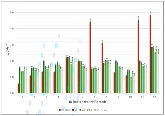
Figure 6.
Luminance values measured on the motorized traffic roads (ID 01 to 12) during the ex-ante and ex-post (C1–C5) measurement campaigns. Error bars report the measurement uncertainty of the ILMD (Image Luminance Measuring Device). The standard requirements of the UNI EN 13201-2 are reported as dotted lines.
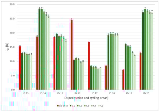
Figure 7.
Illuminance values measured on the pedestrian and cycling areas (ID 13 to 20) during the ex-ante and ex-post (C1–C5) measurement campaigns. Error bars report the measurement uncertainty of the luxmeter. The standard requirements of the UNI EN 13201-2 are reported as dotted lines.
The measured data of both ex-ante and ex-post installations were compared to the standard requirements of the UNI EN 13201-2: 2004 (i.e., the standard in force during the design phase). On motorized traffic roads, the requirements of maintained average luminance were always achieved in the ex-post condition; in ex-ante installations, only 1 case in 12 did not achieve the requirements (requirements satisfied in 92% of cases). Also considering pedestrian areas, the requirements of maintained average horizontal illuminance were always respected both in ex-ante and ex-post installations. As a general comment regarding the comparison with the standard requirements, the measured data referred to different conditions of the luminaires’ maintenance: the ex-ante installations were close to the end of their life, while the ex-post installations were in the first five years of operating life.
Comparing the luminance and illuminance data to the minimum standard requirements, several cases of over-lighting conditions emerged. The issue of the over-illumination of road surfaces is addressed in road lighting standards primarily to avoid energy waste. According to UNI EN 13201-5 [50], the lighting level should not exceed the specified lighting value of the next higher lighting class. In the UNI 11248:2016 [41], it is specified that the maximum acceptable deviation is +35% for M lighting classes and +25% for other lighting classes. The results of the study showed elevated instances of over-illumination in almost all areas and for both ex-ante and ex-post installations. In particular, concerning the luminance measurements conducted in motorized traffic roads, 6 cases of 12 (i.e., 50% of the sample) M lighting categories exceed the requirement by more than 35% in the ex-ante condition. The average percentage of over-illumination for ex-ante installations was +118% (SD 112%) with a maximum of +341%. In the ex-post condition, 10 cases (i.e., 83% of the sample) exceeded the requirement by more than 35%, and the average percentage of over-illumination at C5 was equal to +56% (SD 27%) with a maximum of +103%. In pedestrian areas, seven cases (i.e., 88% of the sample) exceeded the requirement by more than 25% in both ex-ante and ex-post conditions. For ex-ante installations, the average percentage of over-illumination was equal to +121% (SD 68%) with a maximum of +227%, while in the ex-post condition, the average percentage of over-illumination at C5 was equal to +154% (SD 141%) with a maximum of +446%. It should be underlined that a maintenance factor of 0.8 was adopted during the design phase. Consequently, it was foreseeable that when the installations were new, they had values higher by 20–25% than the design value based on standard requirements. The results showed some cases of over-lighting even after 5 years, beyond the expected limits.
Analyzing the data obtained from the five measurement campaigns, irregular trends of the measured parameter (average luminance or illuminance) emerged for many of the areas included in the study. The performance variation between one measurement cycle and the following was in some cases negative (reduction of the photometric performance, as expected) and in other cases positive (increase in the lighting performance), with variations that were often above the measurement uncertainty. This trend was particularly evident for the motorized traffic roads, where the luminance of the pavement was measured to assess the luminous performance of the lighting system. In general, results concerning the pedestrian areas, where illuminance measurements were conducted, showed more regular trends.
4.3. Depreciation of the Photometric Performance
Data from the ex-post LED installations acquired during the five measurement campaigns were further investigated in order to assess the depreciation of the photometric performances over the monitoring period. As described in Section 3.3. the maintenance factor trends obtained from data measured in the field (f′M(L) and f′M(E)) were compared with the predicted maintenance factor trends (fM) calculated based on methods defined in the standards and the literature.
4.3.1. Measured Depreciation of the Photometric Performances
Since the photometric monitoring started after the completion of the lighting systems retrofit, the first measurement campaign (C1) was carried out with a variable delay (from 221 to 8338 operation hours) compared to the LED luminaires’ installation and, therefore, the measured photometric performances of the systems at switch-on time (C0) were not available. To allow for the calculation of f′M(L) and f′M(E) (measured maintenance factor trend) and the comparison with fM (predicted maintenance factor trend), the initial luminance/illuminance values (corresponding to C0) were estimated, for each analyzed motorized traffic road and pedestrian area, through a linear regression of the corresponding C1–C5 measured values.
Figure 8, Figure 9 and Figure 10 report, respectively, the luminance and illuminance values that were measured during the measurement campaigns (C1–C5) and the estimated values corresponding to the first switch-on time, namely the initial performance (C0). The average difference (in operating hours) between C0 and C1 was equal to 5102 h, with a minimum difference of 221 h and a maximum difference of 8338 h.
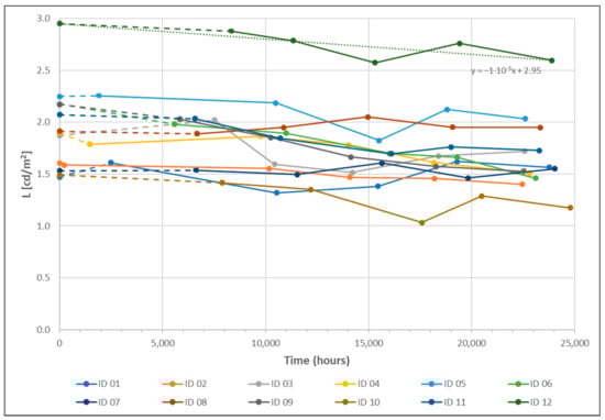
Figure 8.
Measured (C1–C5) and estimated (C0) luminance values of motorized traffic roads (LED01) (i.e., ID 01 to ID 12) over time (in hours). The linear regression was applied to each ID to estimate the initial luminance values at C0 = 0 h and is plotted in the graph as an example (dotted line) for the ID 12.
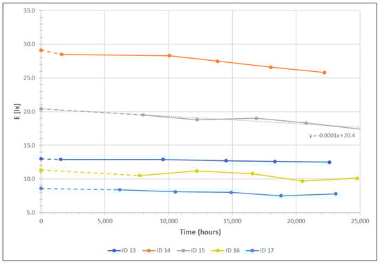
Figure 9.
Measured (C1–C5) and estimated (C0) illuminance values of pedestrian and cycling areas (LED 02) (i.e., ID 13 to ID 17) over time (in hours). The linear regression was applied to each ID to estimate the initial luminance values at C0 = 0 h and is plotted in the graph as an example (dotted line) for the ID 15.
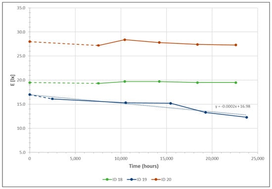
Figure 10.
Measured (C1–C5) and estimated (C0) illuminance values of pedestrian and cycling areas (LED 01) (i.e., ID 18 to ID 20) over time (in hours). The linear regression was applied to each ID to estimate the initial luminance values at C0 = 0 h and is plotted as an example (dotted line) for the ID 19.
To evaluate the maintenance factor over time (f′M(L) and f′M(E)), based on the acquired measured data, the formula of Equation (2) was applied. Figure 11, Figure 12 and Figure 13 report, respectively, the maintenance factor trend of the photometric performance for the considered motorized traffic roads and pedestrian and cycling areas.
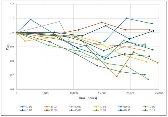
Figure 11.
Maintenance factor (f′M(L)) trends of motorized traffic roads (LED01) (i.e., ID 01 to ID 12).
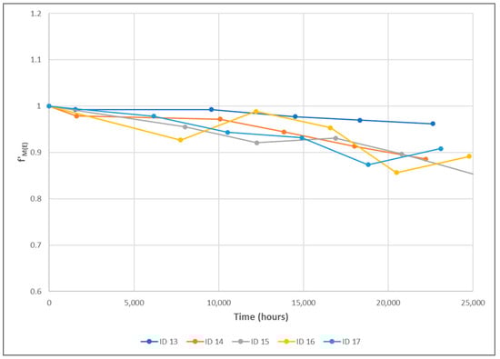
Figure 12.
Maintenance factor (f′M(E)) trends of pedestrian park areas (LED 02) (i.e., ID 13 to ID 17).
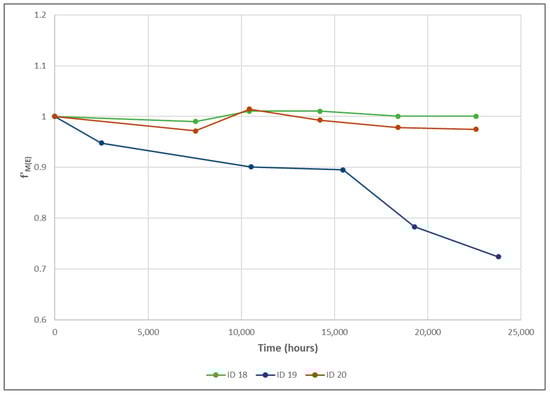
Figure 13.
Maintenance factor (f′M(E)) trends of pedestrian and cyclist areas (LED 01) (i.e., ID 18 to ID 20).
As already outlined in Section 4.2, the data obtained from the five measurement campaigns demonstrated the irregular trends of the measured parameters over time. In Table 6 and Table 7, the percentage variation between one measurement cycle and the previous, and between the last measurement cycle and the switch-on time (C0), are reported. When the luminance values were considered, an increase in lighting with respect to the previous measurement cycle was recorded in 27% of cases, while for illuminance data, this happened in 19% of cases. Furthermore, the average values of the percentage variation between one cycle and the following and the corresponding standard deviation are also lower for illuminance than for luminance values. These results are mainly attributable to the nature of the quantities (illuminance directly related to the luminous flux emitted by the luminaires and luminance related to both the luminous flux of the luminaires and the pavement reflectance) and to the different complexity of the measurement procedures.
Table 6.
Percentage variation between one measurement cycle and the previous, and between the last measurement cycle (C5) and the switch-on time (C0) in motorized traffic roads (luminance measurements).
Table 7.
Percentage variation between one measurement cycle and the previous, and between the last measurement cycle (C5) and the switch-on time (C0) in pedestrian and cyclist areas (illuminance measurements).
Considering the significant variability of the calculated trends, a linear regression analysis was carried out for each of the three sub-samples (motorized and pedestrian areas, with different types of LED). The results of the linear regressions were assumed as representative of the depreciation of the photometric performance (maintenance factor trends) measured in the period C0-C5 for the considered subsets of data. Considering the high dispersion among the measured data, the results of the regression models showed low R2 values, respectively, equal to (i) 0.24, (ii) 0.65 and (iii) 0.18. Figure 14, Figure 15 and Figure 16 show the results of the regression analysis for the considered subsets.
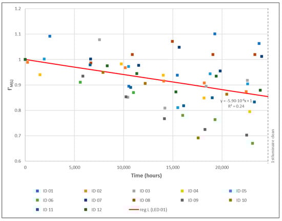
Figure 14.
Regression analysis conducted on measured luminance data in motorized traffic roads (LED01).
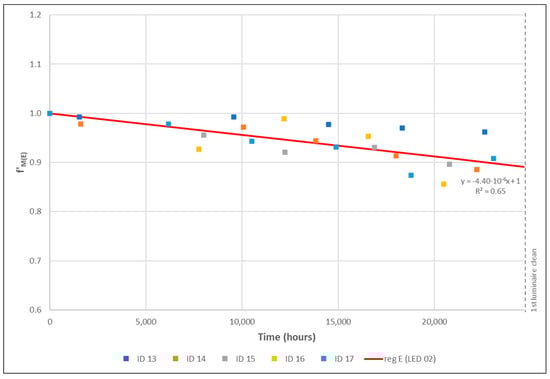
Figure 15.
Regression analysis conducted on measured illuminance data in pedestrian park areas (LED 02).
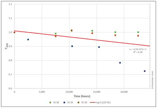
Figure 16.
Regression analysis conducted on measured illuminance data in footpaths and cyclist area (LED 01).
4.3.2. Evaluation of the Predicted Depreciation of the Photometric Performances
The predicted depreciation of the same lighting systems was calculated assuming the maintenance factor calculation method (Equation (3)) in accordance with the standards references, as described in Section 3.3. In particular, considering the terms in the formula, to determine the predicted maintenance factor (fM), the following data were assumed:
- fLF = luminous flux factor—the data of the test conducted in accordance with the LM-80 and the projection generated in accordance with the TM-21, which express the depreciation of the luminous flux over time, were assumed as reported in the datasheet of the LEDs installed in the considered case study.
- fS = survival factor—considering that the replacement of the failed components of the lighting installations was performed immediately with components with similar characteristics, the survival factor (fS) was set to 1.00.
- fLM = luminaire maintenance factor—as specified in Section 3.3., two approaches were used to determine fLM values: the one specified in PD ISO/CIE TS 22012:2019 Annex C.2 [37] and the one reported in BS 5489-1:2020 Annex C1 [38]. For the determination of fLM with the two methods, the following input values were considered:
- (i)
- PD ISO/CIE TS 22012:2019: IP Rating = “IP6X”, as declared in the luminaires datasheet; pollution category = “medium”, based on the environmental characteristics of the case study and the data provided by the ARPA (Regional Agency for Environmental Protection of Piedmont Region) [51].
- (ii)
- BS 5489-1:2020: Environmental zone = “E3/E4”, considering that the analyzed zones were urban areas; mounting heights = “more than 6 metres” in accordance with the geometry of the lighting installations.
- fSM = surface maintenance factor—for outdoor lighting, it only refers to tunnels and underpasses. Since this study includes only outdoor lighting installations, the fSM is set to 1.00.
Based on the data of LED01 and LED02 luminous flux factor (fLF) and on the data of fLM from ISO/CIE and BS standards, four maintenance factor trends were calculated through Equation (3). The calculation was performed assuming an average switch-on period of 4113 h per year and a cleaning interval of 6 years (i.e., 24,678 h). Since for the determination of fLM the [37] standard provides reference values limited to 3 years of exposure time, in this study, the values from 3 to 6 years were derived using linear regression.
The trends of the predicted maintenance factor of the lighting installations with LED01 and LED02, up to the time of the first cleaning interval, are shown in Figure 17 and Figure 18, respectively.
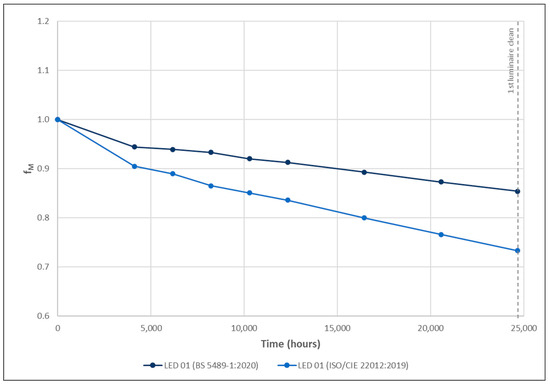
Figure 17.
Predicted maintenance factor (fM) trends considering luminaires equipped with LED01.
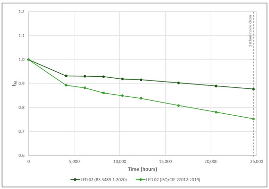
Figure 18.
Predicted maintenance factor (fM) considering luminaires equipped with LED02.
4.3.3. Comparison between Predicted and Measured Depreciation of the Photometric Performance
Finally, the predicted depreciation trends were compared with the measured depreciation. Figure 19, Figure 20 and Figure 21 show the comparison between predicted maintenance factor trends (fM) and the linear regressions assumed as representative of the maintenance factor trends obtained from data measured in the field (f′M) for the three subsets: (i) luminance data, luminaires with LED01 (f′M(L)); (ii) illuminance data with LED02 (f′M(E)); and (iii) illuminance data with LED01 (f′M(E)).
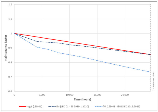
Figure 19.
Comparison between the measured maintenance factor trends of motorized traffic roads (red line) (f′M(L)) and the predicted maintenance factor trends (fM) (dotted lines)—LED01.
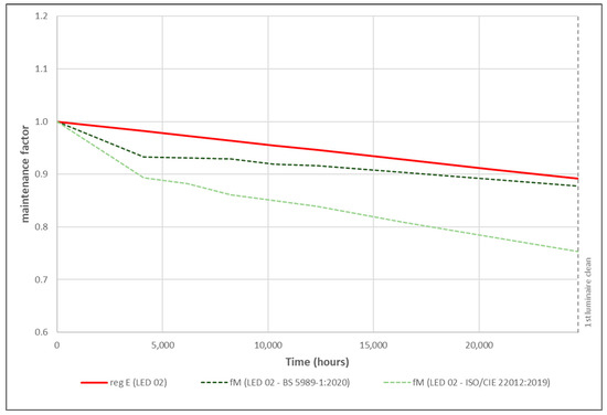
Figure 20.
Comparison between the measured maintenance factor trends of park areas (red line) (f′M(E)) and the predicted maintenance factor trends (fM) (dotted lines)—LED02.
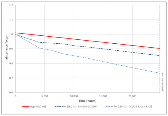
Figure 21.
Comparison between the measured maintenance factor trends of footpaths and cycle path (red line) (f′M(E)) and the predicted maintenance factor trends (fM) (dotted lines)—LED01.
The results demonstrated that the maintenance factor derived from measured data was lower than the predicted maintenance factor calculated according to the reference standards (f′M > fM). In particular, the f′M (which includes both f′M(L) and f′M(E)) trends were in all cases more similar to the fM trend calculated based on the BS 5489-1:2020 fLM data [38]. The percentage variations between the f′M trends and the fM one calculated according to the BS 5489-1:2020 at 24,678 h (first cleaning interval), considering the three subsets, were equal to: 0% (luminance data LED01), 2% (illuminance data LED02) and 4% (illuminance data LED01), respectively. Instead, higher percentage variations were observed by comparing the f′M trend with the fM one calculated according to the PD ISO/CIE TS 22012:2019 [37]: 17% (luminance data LED01), 18% (illuminance data LED02) and 23% (illuminance data LED01), respectively.
5. Discussion
This study reported results on the photometric and energy performances of new LED public lighting systems, installed based on a retrofit project of the previous traditional lighting systems. The study included some significant areas, selected from a larger measured sample. In particular, 20 areas (12 motorized traffic roads and 8 pedestrian and cyclist areas) were selected, based on the observation of the environmental conditions in which the measurements were carried out. In fact, the cases in which the surrounding conditions (e.g., unsuitable weather conditions during the measurement campaigns, changes to the road surface, etc.) highlighted elements of interference or discontinuity between the years of monitoring were excluded from the overall sample.
The energy data acquired by the municipal energy operator and the photometric data measured in field during the measurement campaigns were analyzed to assess the energy and photometric performance of the considered installations and to evaluate the depreciation of the photometric performance of the ex-post lighting systems over time.
Concerning the assessment of the energy performance, an average saving of 51% emerged from the comparison between the ex-ante and ex-post annual energy consumption of the switchboards, which included the lighting installations of the sample considered in this study. The data represented the savings due to the luminaire retrofit (from traditional light sources to LED sources) and the adoption of a night-time luminous flux-reduction program and were in line with results reported in similar studies (see Section 1 “Introduction”). The percentage of saving (51%) was calculated considering only the areas analyzed in this study. Overall, however, the “Torino a LED” project, considering all the luminaires involved in the retrofit (i.e., 54,000 luminaires), allowed for 60% savings for the city.
The assessment of photometric performance was carried out through several measurement campaigns based on the acquisition of illuminance and luminance data. For the motorized traffic roads, luminance data were collected, while illuminance values were acquired in the pedestrian areas. With respect to this aspect, while illuminance is a photometric quantity directly related to the luminous flux emitted by the luminaire, the luminance data also depend on the reflective characteristics of the road surface [52]. In this study, it was not possible to measure the photometric characteristics of the pavements during the measurement campaigns. Therefore, the photometric performances of the motorized traffic roads and their trend throughout the monitoring campaign may have been influenced, rather than by the luminaire depreciation, by the variation of the road surface reflectance due to the aging of the pavement [53,54]. Furthermore, other external conditions could affect the measured illuminance and luminance data [55] and contribute to explaining the non-linear trend of the performances measured over time. Indeed, the in-field monitoring of photometric performances involved a high level of complexity and limitations, which may have influenced the results. Measured data can be affected by obstructions (such as trees and other constructions), nearby ambient lighting (light trespass from advertising, floodlighting, etc.), and environmental conditions (temperature and humidity levels during the in-field measurements). The equipment used and the personnel may also introduce a further level of uncertainty. Moreover, the approach adopted for luminance measurements, i.e., the one provided by the technical international standards EN 13201 part 3 and part 4 [43,44], is quite complex and can lead to mismatches between the measurement points in the different measuring campaigns. As an example, one of the most critical points of the current approach regards the reference observation angle currently used in the standards and the consequent difficulties in making measurements at a 1° observation angle [56]. Therefore, in addition to the lack of information regarding road surface reflectance, the complexity of the measurement method and the difficulties related to the reproducibility of measurements can partially explain the highly variable data over time.
The comparison between the photometric data measured in the field and the standard requirements showed that both in the ex-ante and ex-post conditions the photometric performance satisfies the limits set by the standard. However, as underlined in Section 4.2, some cases of over-illumination emerged, in both motorized traffic roads and pedestrian and cyclist areas and with both ex-ante and ex-post lighting installations. The results showed that in the ex-ante condition, the levels of over-illumination were on average higher, both in the motorized roads and in the pedestrian areas. The over-illumination levels decreased with the LED systems (ex-post condition), but in many cases, they were still higher than the limits set by the standard. The over-illumination of the ex-post installation was calculated after 5 years, and at the end of the sixth year, the cleaning of the luminaires is scheduled; therefore, it can be assumed that the photometric performance of the LED system will return following the cleaning of the luminaires, to values close to the initial ones (net of the depreciation of the light sources). However, it should be considered that the measured performances of the ex-ante condition referred to lighting installations that were close to the end of their life, while the LED systems were in the fifth year of their operating life. Therefore, their performance will be destined to further decrease during their useful life.
Over-illumination can be determined, among other things, by the value of the maintenance factor that is set during the design phase of the lighting installation. Based on this consideration, one of the goals of this study was the assessment of the depreciation of the photometric performance of the LED lighting systems (ex-post installation), based on the photometric data acquired in the field. The determination of the maintenance factor (fM) is an important aspect in the design of a lighting system, in order to properly set up the equipment and the installation to maintain the required photometric performances, while avoiding unnecessary energy consumption. In fact, the maintenance factor reflects the depreciation of the light output of a given installation over time. Nowadays, the calculation models available for determining the fM have only been partially updated with respect to the technological evolution that has occurred in the field of lighting during recent decades. The topic is currently of interest, and numerous research studies are under development at an international level (e.g., within the CIE). In this study, maintenance factor trends were determined based on luminance and illuminance data acquired in the field during a monitoring campaign of approximately 5 years, and they were compared with the predicted maintenance factor trends of the same lighting systems, determined based on the calculation method reported in the main standards in force. The goal was to evaluate the accuracy of the fM calculation methods with respect to the maintenance factor trends measured in the field. The measured illuminance and luminance variation over time, as discussed previously, was quite variable and, therefore, the comparison was conducted with functions obtained from the linear regression of the measured maintenance factor (f′M) trends. As expected, considering the high variability of the measured data, the obtained R2 value was quite low, in particular in the case of luminance data (R2 = 0.18). Moreover, the predicted maintenance factor (fM) trends were determined based on the calculation method proposed by the PD ISO/CIE TS 22012:2019 [37], assumed as the latest practice guidance. Considering the factors of the calculation formula (Equation (3)), both the fS (survival factor) and the fSM (surface maintenance factor) were considered equal to 1 for the characteristics of this study. Consequently, the two factors that influenced the determination of the fM were the fLF (luminous flux factor), which was related to the depreciation of the luminous flux over time of the light source, and the fLM (luminaire maintenance factor), which expressed the relative light output of the luminaire due to dirt deposited. In this study, data on fLF were acquired from manufacturers’ datasheets. However, generally, many difficulties in obtaining these data emerged, increasing the level of difficulty in correctly estimating the fM. Difficulties also emerged in defining the fLM factor, which depends on the dirt deposited on the luminaires. Therefore, as regards the determination of the fLM factor, both the reference values proposed in PD ISO/CIE TS 22012:2019 [37] and in BS 5489-1:2020 [38] were assumed. The calculated fM trends were then compared to the linear regression of the f′M trends obtained from the measured data. The results demonstrated that, for all the considered subsets, the linear regression of the maintenance factor (f′M) at 24,678 h (approximately 5 years, therefore shortly before the first cleaning interval) was close to the predicted level (fM), considering the reference values provided by BS 5489-1:2020 [38]. Instead, greater variations emerged with respect to the maintenance factor (fM) trends defined based on the reference values reported in the PD ISO/CIE TS 22012:2019 [37]. In general, in all the analyzed subsets, the measured maintenance factor (f′M) trends were higher with respect to the predicted ones according to both the considered standards. In other words, the measured depreciation trends of the LED lighting systems were lower with respect to the predicted trends.
Moreover, the predicted maintenance factor (fM) showed a non-linear trend with respect to the first year of life (significant difference between fM values at t = 0 and t = 1 year of life). These trends were determined by the fLF reference values provided by the standards. Therefore, according to the predicted maintenance factor (fM) trends, the lighting installations would suffer a greater depreciation during the first year of life. In this study, it was not possible to verify this aspect through the measured maintenance factor (f′M) trends, as the measurement intervals between the measuring campaigns were not regular and therefore the data measured at 1 year of life were not available.
6. Conclusions
The study presented in this paper was aimed at assessing and monitoring the performances of LED public lighting systems, based on a retrofit project of the previous traditional lighting systems. A method was set up to assess and compare the performances of the ex-ante (traditional luminaires) and ex-post (LED) lighting systems, in order to evaluate both energy performances (data acquired from the remote-control system) and photometric performances (data from in-field measuring campaigns). Moreover, the study involved the assessment of the depreciation of the photometric performance of the ex-post installations over a period of about 5 years (based on measured data) and comparison with the predicted depreciation (estimated based on the calculation method proposed by the main standards currently in force).
In the study, the proposed method was applied to a significant sample of roads and pedestrian areas included in the lighting renovation program of the city of Turin (Italy). Results showed that:
- The retrofit project, and therefore the adoption of more efficient technologies as well as a control system to dim the light during night-time, allowed for significant energy savings, equal to a 51% reduction in annual energy consumption in the considered areas;
- The new LED system complied with the requirements imposed by the standard in force. Furthermore, the new lighting system allowed for improving critical issues related to the over-illumination of some areas, avoiding energy waste as well as reducing the environmental impact;
- By monitoring the performance of the new LED system over a period of 5 years, it was possible to determine the measured depreciation of the photometric performance, based on in-field measurements;
- The comparison of the measured depreciation with the predicted one (based on the maintenance factor calculation method) showed that the measured depreciation was lower than the predicted one. Furthermore, it was possible to observe that, among the standards considered, the predicted maintenance factor trends defined according to the reference data provided by BS 5489-1:2020 [38] were closer to the measured one. Instead, more variation emerged with respect to the predicted maintenance factor trends defined according to reference values provided by the PD ISO/CIE TS 22012:2019 [37].
The presented study suffers from some limitations, mainly related to external conditions that could influence the measured data. In particular, concerning luminance data, the reflective characteristics of the road surface were not considered, and future efforts may be directed toward implementing this aspect.
Despite some limitations, the study reported results of long-term monitoring based on measured data (while previous studies were mainly focused on forecast estimates) and allowed us to define useful considerations with respect to the depreciation of LED lighting systems that may be useful within the design phase, to properly assess the maintenance factor. Indeed, designing with appropriate reference values for calculating the fM is crucial to avoid oversizing the lighting systems. Over-lighting can have many negative impacts: excessive and useless energy consumption, negative impact on light pollution with potential consequences on the well-being of humans and ecosystems, and environmental impacts.
The results obtained in this study showed that the measured depreciation of the photometric performance during the first 5 years of life of the considered lighting installations was closer to the predicted depreciation trend defined according to BS 5489-1:2020 (variations between 0% and 4%). Instead, significant variations (between 17% and 23%) emerged considering the ISO/CIE TS 22012:2019. As shown in the Methods section, the two standards are based on the same calculation method for determining the maintenance factor but differ in the reference values provided in determining the fLM (luminaire maintenance factor), which expresses the relative output of the luminaire due to dirt deposited. According to the results of the study, considering the reference values of the BS 5489-1:2020 to determine the fLM (luminaire maintenance factor), and therefore the predicted maintenance factor trends, in the design phase would be more appropriate.
The results presented in this study are limited to the sample installations considered as a case study; therefore, additional efforts would be needed to extend the proposed methodology to a larger sample and to obtain generalizable results. However, the obtained results could be useful in order to define indications to properly size the lighting systems, avoiding unnecessary energy consumption and limiting the environmental impact.
Author Contributions
Conceptualization, A.P.; methodology, A.P., L.V., G.P. and R.T.; formal analysis, L.V., G.P. and R.T.; investigation, A.P., G.P. and R.T.; data curation, L.V, G.P. and R.T.; writing—original draft preparation, L.V., G.P. and R.T.; writing—review and editing, L.V. and A.P.; supervision, A.P.; project administration, A.P.; funding acquisition, A.P. All authors have read and agreed to the published version of the manuscript.
Funding
This research was funded by IREN Smart Solution S.p.A. (IT).
Institutional Review Board Statement
Not applicable.
Informed Consent Statement
Not applicable.
Data Availability Statement
Data are available upon request.
Acknowledgments
The study was carried out within a research project between the Department of Energy of the Politecnico di Torino and IREN Smart Solution S.p.A. The authors acknowledge IREN Smart Solution for the data provided for the study and booth IREN Smart Solution and the City of Turin for the support given during the in-field monitoring campaigns.
Conflicts of Interest
The authors declare no conflict of interest.
References
- Peña-García, A.; Hurtado, A.; Aguilar-Luzón, M.C. Impact of public lighting on pedestrians’ perception of safety and well-being. Saf. Sci. 2015, 78, 142–148. [Google Scholar] [CrossRef]
- Fotios, S.A.; Robbins, C.J.; Farrall, S. The Effect of Lighting on Crime Counts. Energies 2021, 14, 4099. [Google Scholar] [CrossRef]
- Seshadri, K. City beautification at night. J. Illum. Eng. Inst. Jpn. 1997, 81, 139–140. [Google Scholar] [CrossRef] [PubMed]
- Boyce, P.R. The benefits of light at night. Build. Environ. 2019, 151, 356–367. [Google Scholar] [CrossRef]
- CIE 234:2019; A Guide to Urban Lighting Masterplanning. CIE Technical Report: Wien, Austria, 2019. [CrossRef]
- Traverso, M.; Donatello, S.; Moons, H.; Rodriguez Quintero, R.; Gama Caldas, M.; Wolf, O.; Van Tichelen, P.; Van Hoof, V.; Geerken, T. Revision of the EU Green Public Procurement Criteria for Street Lighting and Traffic Signals; Publications Office of the European Union: Luxembourg, 2017. [Google Scholar] [CrossRef]
- Bachanek, K.H.; Tundys, B.; Wiśniewski, T.; Puzio, E.; Maroušková, A. Intelligent street lighting in a smart city concepts. A direction to energy saving in cities: An overview and case study. Energies 2021, 14, 3018. [Google Scholar] [CrossRef]
- Zissis, G.; Bertoldi, P.; Serrenho, T. Update on the Status of LED-Lighting World Market Since 2018; Publications Office of the European Union: Luxembourg, 2021. [Google Scholar] [CrossRef]
- Cellucci, L.; Burattini, C.; Drakou, D.; Gugliermetti, F.; Bisegna, F.; Vollaro, A.D.L.; Salata, F.; Golasi, I. Urban lighting project for a small town: Comparing citizens and authority benefits. Sustainability 2015, 7, 14230–14244. [Google Scholar] [CrossRef]
- Griffiths, H. The Future of Street Lighting: The Potential for New Service Development; IoT UK; Future Cities Catapult: London, UK, 2017; Available online: http://iotuk.org.uk/wp-content/uploads/2017/04/The-Future-of-Street-Lighting.pdf (accessed on 1 May 2023).
- Kostic, M.; Djokic, L. Recommendations for energy efficient and visually acceptable street lighting. Energy 2009, 34, 1565–1572. [Google Scholar] [CrossRef]
- Donatello, S.; Rodriguez Quintero, R.; Gama Caldas, M.; Wolf, O.; Van Tichelen, P.; Van Hoof, V.; Geerken, T. Revision of the EU Green Public Procurement Criteria for Road Lighting and Traffic Signals; Publications Office of the European Union: Luxembourg, 2019. [Google Scholar] [CrossRef]
- Available online: https://www.iea.org/about (accessed on 1 May 2023).
- Lighting Europe. Strategic Roadmap 2025 of the European Lighting Industry. Available online: https://www.lightingeurope.org/media/34-roadmap-of-human-centric-lighting (accessed on 1 May 2023).
- Tavares, P.; Ingi, D.; Araújo, L.; Pinho, P.; Bhusal, P. Reviewing the Role of Outdoor Lighting in Achieving Sustainable Development Goals. Sustainability 2021, 13, 12657. [Google Scholar] [CrossRef]
- Pardo-Bosch, F.; Blanco, A.; Sesé, E.; Ezcurra, F.; Pujadas, P. Sustainable strategy for the implementation of energy efficient smart public lighting in urban areas: Case study in San Sebastian. Sustain. Cities Soc. 2022, 76, 103454. [Google Scholar] [CrossRef]
- Pagden, M.; Ngahane, K.; Amin, M.S.R. Changing the colour of night on urban streets—LED vs. part-night lighting system. Socio-Econ. Plan. Sci. 2020, 69, 100692. [Google Scholar] [CrossRef]
- De Almeida, A.; Santos, B.; Paolo, B.; Quicheron, M. Solid state lighting review. Potential and challenges in Europe. Renew. Sustain. Energy Rev. 2014, 34, 30–48. [Google Scholar] [CrossRef]
- Weisbuch, C. Historical perspective on the physics of artificial lighting. Comptes Rendus Phys. 2018, 19, 89–112. [Google Scholar] [CrossRef]
- Tähkämö, L.; Ylinen, A.; Puolakka, M.; Halonen, L. Life cycle cost analysis of three renewed street lighting installations in Finland. Int. J. Life Cycle Assess. 2012, 17, 154–164. [Google Scholar] [CrossRef]
- Tähkämö, L.; Halonen, L. Life cycle assessment of road lighting luminaires—Comparison of light-emitting diode and high-pressure sodium technologies. J. Clean. Prod. 2015, 93, 234–242. [Google Scholar] [CrossRef]
- Beccali, M.; Bonomolo, M.; Ciulla, G.; Galatioto, A.; lo Brano, V. Improvement of energy efficiency and quality of street lighting in South Italy as an action of Sustainable Energy Action Plans. The case study of Comiso (RG). Energy 2015, 92, 394–408. [Google Scholar] [CrossRef]
- Campisi, D.; Gitto, S.; Morea, D. Economic feasibility of energy efficiency improvements in street lighting systems in Rome. J. Clean. Prod. 2018, 175, 190–198. [Google Scholar] [CrossRef]
- Picardo, A.; Galván, M.J.; Soltero, V.M.; Peralta, E. A Comparative Life Cycle Assessment and Costing of Lighting Systems for Environmental Design and Construction of Sustainable Roads. Buildings 2023, 13, 983. [Google Scholar] [CrossRef]
- Gil-De-Castro, A.; Moreno-Munoz, A.; Larsson, A.; de La Rosa, J.J.G.; Bollen, M.H.J. LED street lighting: A power quality comparison among street light technologies. Light. Res. Technol. 2013, 45, 710–728. [Google Scholar] [CrossRef]
- Djuretic, A.; Kostic, M. Actual energy savings when replacing high-pressure sodium with LED luminaires in street lighting. Energy 2018, 157, 367–378. [Google Scholar] [CrossRef]
- Gorgulu, S.; Kocabey, S. An energy saving potential analysis of lighting retrofit scenarios in outdoor lighting systems: A case study for a university campus. J. Clean. Prod. 2020, 260, 121060. [Google Scholar] [CrossRef]
- Life-DIADEME, Sustainable Smart Lighting System, Project Co-Financed by EU. Available online: https://www.diademe.it/ (accessed on 15 June 2023).
- Di Lecce, P.; Mazzocchi, A.; Rossi, G. Outdoor Adaptive Lighting in the New UNI 11248 Italian Standard and Result of Experience. In Proceedings of the Lux Europa, Ljubljana, Slovenia, 18–20 September 2017. [Google Scholar]
- Valetti, L.; Floris, F.; Pellegrino, A. Renovation of public lighting systems in cultural landscapes: Lighting and energy performance and their impact on nightscapes. Energies 2021, 14, 509. [Google Scholar] [CrossRef]
- Beccali, M.; Bonomolo, M.; Lo Brano, V.; Ciulla, G.; Di Dio, V.; Massaro, F.; Favuzza, S. Energy saving and user satisfaction for a new advanced public lighting system. Energy Convers. Manag. 2019, 195, 943–957. [Google Scholar] [CrossRef]
- Yoomak, S.; Jettanasen, C.; Ngaopitakkul, A.; Bunjongjit, S.; Leelajindakrairerk, M. Comparative study of lighting quality and power quality for LED and HPS luminaires in a roadway lighting system. Energy Build. 2018, 159, 542–557. [Google Scholar] [CrossRef]
- Beccali, M.; Bonomolo, M.; Galatioto, A.; Pulvirenti, E. Smart lighting in a historic context: A case study. Manag. Environ. Qual. Int. J. 2017, 28, 282–298. [Google Scholar] [CrossRef]
- Leccese, F.; Salvadori, G.; Rocca, M. Critical analysis of the energy performance indicators for road lighting systems in historical towns of central Italy. Energy 2017, 138, 616–628. [Google Scholar] [CrossRef]
- Ogando-Martínez, A.; López-Gómez, J.; Febrero-Garrido, L. Maintenance Factor Identification in Outdoor Lighting Installations Using Simulation and Optimization Techniques. Energies 2018, 11, 2169. [Google Scholar] [CrossRef]
- Mockey Coureaux, I.O.; Manzano, E. The energy impact of luminaire depreciation on urban lighting. Energy Sustain. Dev. 2013, 17, 357–362. [Google Scholar] [CrossRef]
- PD ISO/CIE TS 22012:2019; Light and lighting. Maintenance Factor Determination. Way of Working. International Organization for Standardization: Brussels, Belgium, 2019.
- BS 5489-1:2020; Code of Practice for the Design of Road Lighting Part 1: Lighting of Roads and Public Amenity Areas. British Standards Institution (BSI): London, UK, 2020.
- Città di Torino. Piano Urbano del Traffico [Urban Traffic Plan]. 2001. Available online: https://www.comune.torino.it/put2001/ (accessed on 15 June 2023).
- Città di Torino, IRIDE Servizi. Piano Regolatore dell’Illuminazione Comunale (PRIC) [Municipal Lighting Regulatory Plan]. 2011. Available online: http://www.comune.torino.it/canaleambiente/pric/ (accessed on 15 June 2023).
- UNI 11248:2012; Illuminazione Stradale. Selezione Delle Categorie Illuminotecniche. UNI: Rome, Italy, 2012.
- EN 13201:2015; Road Lighting. European Committee for Standardization (CEN): Belgium, Brussels, 2015.
- EN 13201-3:2015; Road Lighting. Part 3: Calculation of Performance. European Committee for Standardization (CEN): Belgium, Brussels, 2015.
- EN 13201-4:2015; Road Lighting. Part 4: Methods of Measuring Lighting Performance. European Committee for Standardization (CEN): Belgium, Brussels, 2015.
- EN 13201-2:2015; Road Lighting. Part 2: Performance Requirements. European Committee for Standardization (CEN): Belgium, Brussels, 2015.
- CIE 194:2011; On Site Measurement of the Photometric Properties of Road and Tunnel Lighting. CIE Technical Report: Wien, Austria, 2011.
- Tomczuk, P.; Chrzanowicz, M.; Jaskowski, P.; Budzynski, M. Evaluation of Street Lighting Efficiency Using a Mobile Measurement System. Energies 2021, 14, 3872. [Google Scholar] [CrossRef]
- IES LM-80-08; Approved Method for Measuring Lumen Maintenance of LED Light Source. IES: New York, NY, USA, 2008.
- IES TM-21-11; Projection Long Term Lumen Maintenance of LED Light Sources. IES: New York, NY, USA, 2011.
- EN 13201-5:2015; Road Lighting. Part 5: Energy Performance Indicators. European Committee for Standardization (CEN): Belgium, Brussels, 2015.
- ARPA Piemonte. Available online: https://www.arpa.piemonte.it/ (accessed on 15 June 2023).
- Gidlund, H.; Lindgren, M.; Muzet, V.; Rossi, G.; Iacomussi, P. Road Surface Photometric Characterisation and Its Impact on Energy Savings. Coatings 2019, 9, 286. [Google Scholar] [CrossRef]
- Florian, G.; Boucher, V.; Dronneau, R.; Muzet, V. Design of an adaptive road lighting installation taking into account the evolution of pavement reflection properties according to the weather conditions. In Proceedings of the Lux Europa, Prague, Czech Republic, 20–22 September 2022. [Google Scholar]
- Muzet, V.; Liandrat, S.; Bour, V.; Dehon, J.; Christory, J.P. Is it possible to achieve quality lighting without considering the photometry of the pavements? In Proceedings of the Conference CIE 2021, NC Malaysia online, 27–29 September 2021. [Google Scholar] [CrossRef]
- Bouroussis, C.A.; Gašparovský, D. A holistic method for the commissioning and optimisation of adaptive road lighting systems using field measurements. In Proceedings of the Conference CIE 2021, NC Malaysia online, 27–29 September 2021. [Google Scholar] [CrossRef]
- Muzet, V.; Bernasconi, J.; Iacomussi, P.; Liandrat, S.; Greffier, F.; Blattner, P.; Reber, J.; Lindgren, M. Review of road surface photometry methods and devices—Proposal for new measurement geometries. Light. Res. Technol. 2021, 53, 213–229. [Google Scholar] [CrossRef]


Disclaimer/Publisher’s Note: The statements, opinions and data contained in all publications are solely those of the individual author(s) and contributor(s) and not of MDPI and/or the editor(s). MDPI and/or the editor(s) disclaim responsibility for any injury to people or property resulting from any ideas, methods, instructions or products referred to in the content. |
© 2023 by the authors. Licensee MDPI, Basel, Switzerland. This article is an open access article distributed under the terms and conditions of the Creative Commons Attribution (CC BY) license (https://creativecommons.org/licenses/by/4.0/).