Scenario Analysis of Offshore Wind-Power Systems under Uncertainty

Abstract

Wind-energy systems are strongly affected by uncertainty and variability. Therefore, uncertainty sources should be considered during the economic evaluation of this type of system. In the literature, a framework for the economic performance assessment of wind-power systems has been proposed. Furthermore, in another contribution, the random discontinuities of political and regulatory scenarios have been included by using scenario analysis. However, the implemented models neglected the uncertainty related to disruptive events and the effect of climate change on the wind resource. To fill this gap, in this paper, climate change and disruptive events are included in a new model for evaluating the economic performance of wind turbine systems using scenario analysis. Analysis of a numerical example has been carried out to show the framework’s capabilities and to evaluate the effects of the added issues. The main results confirm previous findings on the necessity of including regulatory and political risks to achieve a proper economic evaluation. Additionally, they show that disruptive events increase the variability of the expected value of the Net Present Value (NPV). Therefore, even though climate change is expected to increase wind producibility in the numerical example location, the inclusion of disruptive events constrains the NPV growth.

1. Introduction

Renewable energy power systems (RESs) are crucial for the decarbonisation goal, and energy transition policies represent one of the main tools against climate change and for achieving energy independence. Engineering progresses in RESs have been reducing the levelised cost of energy (LCOE) extracted by green resources, and it has become comparable with the LCOE of fossil sources. However, RESs’ profitability is affected by many aleatory and epistemic uncertainty sources, increasing the investment and financial risks [1]. This work focuses on wind-power systems, which are representative green energy systems. Onshore wind-power systems are widespread, and the effect of wind-speed changes, electricity price variability, and random failures have been investigated in the literature [2,3,4]. The variability of the wind speed establishes several problems in the wind turbine control [5], and particular attention should be paid during the design phase of the supporting structure to reduce their uncertainties under emergency conditions [6]. The epistemic uncertainty of imprecise turbine design formulas and the effects on the onshore systems’ performance of disruptive external events due to natural and man-made hazards are also well-known. Tozzi and Jo (2017) [7] reviewed available software tools for evaluating the performance of onshore wind-power systems [8,9,10]. Despite that, most existing tools consider the uncertainty using sensitivity analysis while changing one element at a time. Moreover, often, only a few sources of uncertainty are considered. However, the case of offshore wind-power plants differs from that of onshore ones, and the uncertainty and variability effect in this type of system have not been fully investigated.

Recently, a model has been proposed to estimate the performance of offshore wind-power systems, including simultaneously epistemic and random uncertainty, to assess the probability density function of the NPV [11]. In another work, the uncertainty of changes in the political and regulatory scenario during the system’s life was included [12]. The authors considered several widely accepted scenarios related to energy price history, the learning rate of offshore wind-power systems, and subsidies policy and combined them to include these additional risks. However, the effect of disruptive events and climate change on the NPV has been neglected. To fill this gap, in this paper, the previously available model [11,12] is extended by including climate change’s impact on wind speed and ship collisions to consider disruptive events. Furthermore, the scenarios’ construction and the so-called scenario combination procedure are carefully described.

The paper is organised as follows. Firstly, the literature on the existing framework for evaluating the economic performance of wind-energy systems, ship collisions with offshore wind turbines, climate-change effects on wind-power systems, and scenario analysis is analysed. After that, the technical and economic model and the uncertainty propagation method are briefly described. Subsequently, the approaches for including disruptive events and climate change effects are exposed. Next, the adopted scenarios and their combination methodology are explained. Then, the relevance of considering scenarios, the impact of ship collisions, and future wind-speed forecasts in the economic performance evaluation of wind-power systems is shown by carrying out a numerical example. Finally, four scenarios are combined to include random discontinuities of the subsidy policy, using their associated probabilities and estimating a single NPV distribution. The combination results are compared to the case of random discontinuity absence to understand if the efforts to estimate the probability are justified by different economic performances.

2. Literature Review

The literature focused on the evaluation of offshore wind-power systems under uncertainty has been reviewed elsewhere [11,12]. However, some relevant contributions are summarised below.

The modelling of wind-energy systems focusing on technical and economic models but neglecting uncertainty has been studied in recent years [13,14]. Nevertheless, the uncertainty of wind speed strongly influences the economic performance of the wind turbines, and the inclusion of that significantly improves the evaluation accuracy [15,16]. Although the economic model suffers from the effects of wind speed, its technical performance is influenced too. Therefore, when only the technical model is built, its inclusion impacts the final evaluation [17,18]. The epistemic uncertainty of the technical model is another crucial aspect of the evaluation problem. Indeed, wind-power forecasting [19], the non-perfect knowledge of the power curve [20], manufacturing tolerances, and events like insect contamination [21] may impact the results of the viability analysis. Furthermore, other critical epistemic uncertainty sources have been considered in the literature, like the wake effect, the internal wind farm collector system, and the unavailability of wind turbines [22].

Additionally, another uncertainty source that may radically change the feasibility of the investment is represented by failures, which should be modelled [23,24,25,26,27,28].

When the economic model is involved, modelling the energy price variability is a relevant issue. Recently, a framework that models the energy price and wind-speed variability, while also accounting for power curve epistemic uncertainty, has been proposed [29].

Finally, a comprehensive framework has been developed by attempting to include several sources of aleatory and epistemic uncertainty [11].

From commercial computer tools for evaluating renewable energy systems’ perspectives, some interesting items are available [8,9,10,30]. However, these pieces of software have certain limitations in considering some sources of uncertainty or in adopting some techniques for their modelling.

Since this work aims to include ship collision events and climate-change effects on wind-power systems and to formalise the scenario analysis procedure, the literature on these topics is provided below.

Some papers in the literature have focused on the ship collision analysis on offshore wind turbines. The majority of works have considered fixed-bottom structures. Indeed, monopile foundations for offshore wind turbines’ response to ship collision have been tested both with a striking rigid-body ship and a deformable body [31]. The deformation of the jacket foundation under a ship collision has been considered by including different scenarios of the ship’s speed, collision direction, and angle [32]. The ship collision may cause plastic deformation, leading to wind-turbine collapse [31,32]. The effects of collision increase when the wind load is considered in the analysis, reducing the impact energy needed for the turbine’s collapse [33]. The risk of collision is higher when considering service vessels during maintenance operations. Even if the vessel speed is low, the wind-turbine structure can be affected by the impact, resulting in structural damage [34]. Considering the impact between vessels and wind turbines, 20% of the ship–turbine strikes occur on approach, while 80% occur on drift [34]. Therefore, this means that 80% of collisions happen at a speed of 0.3–2.8 m/s. Indeed, the most frequent speed is 1.2 m/s. The relevance of offshore maintenance in fixed-bottom wind turbines has been extensively reviewed [35]. Therefore, the risk of collision with a maintenance vessel increases due to the high number of interventions. In the literature, the collision of a barge and a bulk ship with different loads with a fixed-bottom offshore wind turbine has been investigated, and the combination of the results allows researchers to provide two fragility curves, one for each type of ship [36]. The driving factor of the fragility curves is the current speed of the ship at the strike. When considering floating offshore wind turbines, the literature is scarce. In recent years, intending to fill this gap, an initial step for analysing the effects of ship collision on a spar-floating offshore wind turbine has been proposed [37]. As per the findings, the mass and the initial velocity are lead factors in the deformation process. Furthermore, there is an elastic response of the overall structure, which reduces the total effect of the impact in comparison with a fixed-turbine type at the same speed. For the floating spar, a strike at a speed of about 5 m/s may seriously damage the system. Indeed, the failure analysis of a spar buoy structure shows that a crash with vessel is a relevant event, with a probability of about 10⁻⁶ events per hour. The consequences of these events have been considered severe. The dynamic and damage analyses carried out in a recent paper allow us to understand how severe the consequences of the collision of a ship with a spar buoy are [38]. Finally, the combination of collision load and wind wave-mooring loads has been investigated [39]. The analysis of the literature suggests that:

• The ship collision impacts floating structures less than bottom-fixed ones.
• The wind and wave loads decrease the critical speed, leading to the wind turbine’s collapse.
• Most collisions happen between small service vessels with a load ranging from 125 to 850 tons. Collision with a bulk ship with a mass of 30,000 tons is rarer but may happen.
• Approximately 20% of the collisions happen on approach at high speed, while most happen on drift at a low speed in the range of 0.3–2.8 m/s.
• Collision at speeds higher than 5–6 m/s may be critical and can damage the spar structure.
• Only fragility curves for ship collisions between barge and bulk ships and fixed-bottom structures are available in the literature.

Climate change affects weather conditions, and the fact that renewable energy systems suffer from this issue is well known. Wind-energy systems are one of the instruments used to mitigate climate change and produce green energy. However, wind-energy systems suffer from climate evolution, and climate change may negatively impact wind farm production. Indeed, in the future, some regions of the world may experience a reduced wind speed, whereas others may experience an increase. An in-depth review of climate change’s impact on wind energy has been proposed in the literature [40]. The authors focused on the variability of the wind resource in northern Europe, considering also the effects of climate change on the maintenance of wind farms. Indeed, they considered extreme wind speed, icing, sea ice and permafrost, and also air density. The wind speed will increase in some regions of north and central Europe, but undesirable weather-critical events will also increase [40]. Considering changes in wind speed and direction at 10 m worldwide due to the anthropogenic climate change, global warming impacts the future of the wind resource. In the future, there will be a possible increase in the probability of extreme wind speed due to tropical cyclones [41]. However, further studies are required. A recent work studied the evolution of wind speed in Chile to evaluate its impact on optimal power-system expansion plans [42]. They analysed scenarios of three different concentrations of greenhouse gasses and concluded that even though the mean wind speed will slightly increase in the next few years, its variability will increase too. Another work analysed in depth the future wind-speed probability distribution [43]. The authors resorted to several circulation models and simulated wind speed at 10 m under the representative concentration pathway (RCP) 8.5 condition. The RCP 8.5 scenario supposes that emissions will continue to increase during the 21st century. It is often taken as the worst-case climate-change scenario. It hypothesises that the global mean temperature will increase by 5 °C in 2100 compared with its value in the pre-industrial era. The sea level will also increase by about 0.63 m [44,45]. The simulation of the near-surface wind speed showed that the most significant wind-speed decrease will be in Eastern Russia and the USA. The authors’ analysis provided the fitting distribution, accuracy, mean value, and standard deviation of the current wind speed and the simulated wind speed in the near, midterm, and far future. Even though in some world regions wind-speed changes will be marginal, a slight change strongly affects the extracted power from the wind. Since the wind turbine of the numerical example is located in Italy, a study on the impacts of climate change on power generation in Italy is considered [46]. The paper studied wind-resource availability in Italy for the short (until 2050), medium (until 2080), and long (until 2100) term. Two scenarios were analysed: the RCP 8.5 and the RCP 4.5. The RCP 4.5 supposes that the emissions peak in 2040 and then decline. It is often considered the most probable baseline scenario in which the increases in temperature in 2100 will be about 2.5–3 °C, and the sea level increases by about 0.47 m compared with the data from the pre-industrial baseline. They assessed wind producibility as the ratio between the produced power per hour and the installed power. The results showed that in both scenarios, the wind producibility will increase in the short period in the plant region of the numerical study by about 3–4%. However, in other regions of Italy, the producibility will decrease.

In the literature, scenario planning is a widely adopted approach to explore the possible evolutions of macroscopic variables over medium and long time horizons. As a matter of fact, several reviews are available on this topic [47,48,49]. This approach focuses on the complexity and uncertainty of the environment. Indeed, its primary goal is not to forecast variables’ values but to depict several different futures. The uses of scenario planning rely on defining plausible and possible descriptions of the future. Even though various methods exist, most of them imply a high level of subjective judgement. Therefore, the scenario-making process often has low replicability. Indeed, all three of the most important techniques of scenarios, that is, Intuitive logic methodology, La prospective methodology, and Probabilistic modified trends methodology, are based on experts’ judgements [50]. Generally, scenarios are produced by analysing reality and identifying the most influential variables on future developments. Then, it is crucial to determine the driving forces that cause changes in the future influential variables. Basically, the scenario planning includes the following steps:

• Defining the objective of the study. The output of this step is the system selection, the study’s time horizon, the geographic boundaries, and the stakeholders.
• Collecting data. Resorting to the specifications obtained in step 1, the data collection about all the relevant issues necessary to describe the events affecting the factors and variables that lead to future developments are collected.
• Understanding trends and uncertain elements. The identified factors and variables are studied to understand their influence on the system under analysis, the range of their variability over time, and trends. Additionally, their number is streamlined by conducting uncertainty analysis or similar approaches.
• Understanding the interdependence between the events, factors, and variables value. This step is crucial to understand whether and how one variable affects another. This way, one can suppose a correlation matrix, which transparently defines the probability of another event or a value once one has happened.
• Building the scenarios. Combining different trends and uncertainty allows us to describe several scenarios, which are then reduced in number using expert judgements and available data, establishing a subjective procedure.

Analysts and decision makers often adopt strategies to cope with the consequences of realising different scenarios. For the sake of completeness, more quantitative approaches to scenario planning also exist. These are based mainly on the combination of analytical formulation, sampling methods, and the contribution of experts. For instance, the Interactive Cross Impact Simulation uses Monte Carlo simulation, combining data and experts’ opinions [51]. On the other hand, Trend impact analysis resorts to historical trend interpolation and opinions to set the probabilities and impacts of future events [52].

Steps 2 and 3 are often carried out using cause–effect analysis [53,54]. This approach often gives a cause–effect matrix, in which the rows are the variables, whereas the columns are the outputs. In the intersections, there is a qualitative or quantitative measure of the effect that a variable has on the output.

Step 4 often uses the cross-impact analysis, a widely adopted tool for understanding the interdependence between events [55,56]. It is used to analyse if and how much the occurrence of an event influences the probability of the occurrence of another event. Typically, the output of the procedure is a cross-impact matrix. The cross-impact matrix is a matrix in which each row and each column represent a variable. In the intersections is a qualitative or quantitative value describing the interdependence level. The qualitative value can be, for instance, a plus, neutral, or minus symbol. In contrast, the quantitative measure can be the value of the reduction in the probability of occurrence of the event in the column once the event in the row has occurred. This approach allows futurists to build consistent and plausible scenarios.

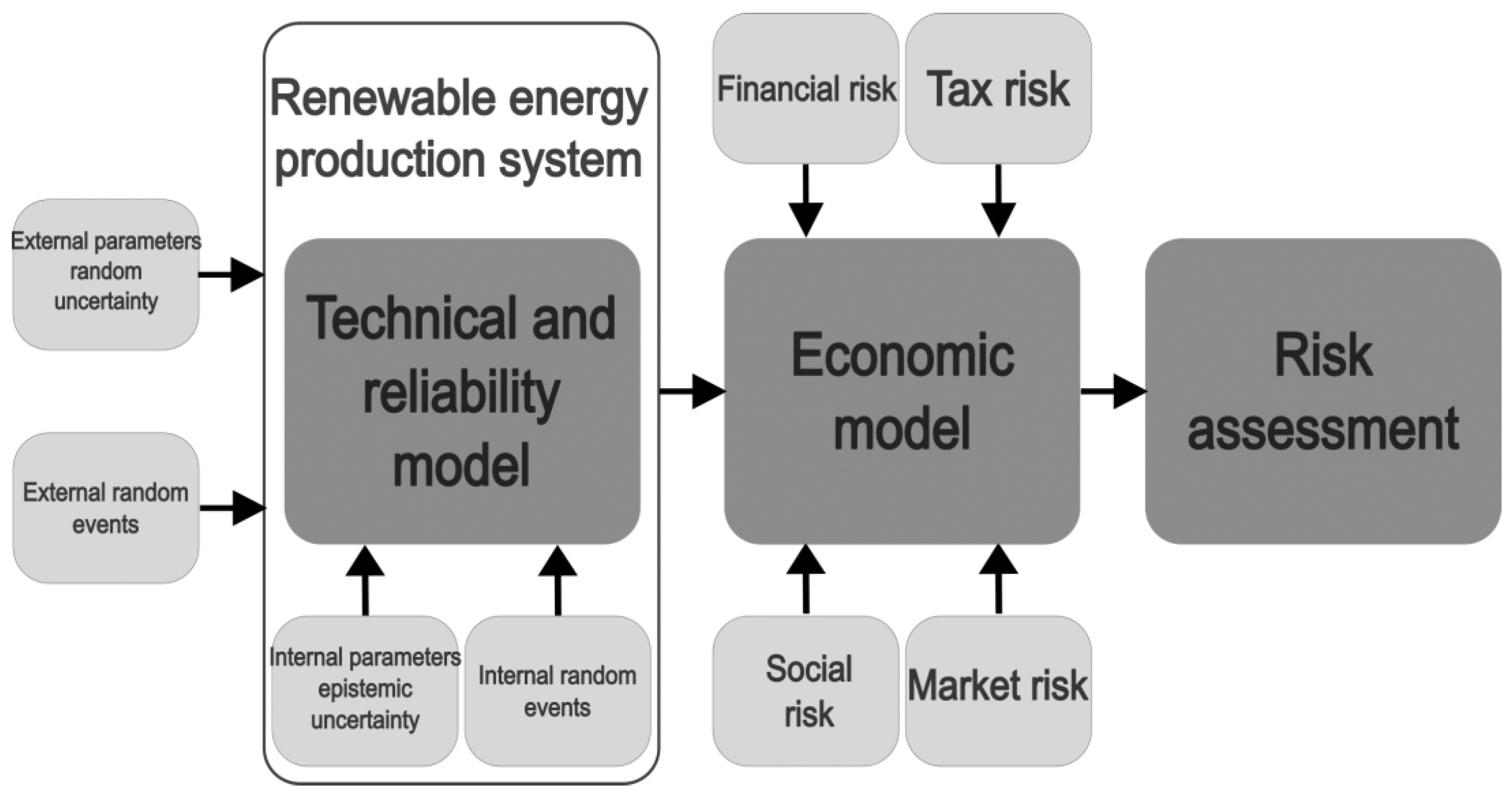
3. Framework for Uncertainty Propagation and Risk Assessment

The framework for uncertainty propagation and risk assessment (Figure 1) comprises modular blocks, which can be added and removed to represent several sources of uncertainty.

In this paper, the wind-power system suffers from the uncertainty sources summarised in

Table 1. Sources of uncertainties.

Variable	Uncertainty Nature/ Variability Type	Modelling Approach
Bank interest rate	E/II	1
Investment cost	E/II	1
Plant nominal life	E/II	1
Self-interest rate	E/II	1
Power coefficient	E/II	1
Gearbox efficiency	E/II	1
Generator efficiency curve	E/II	2
Power electronic efficiency curve	E/II	2
Number of required maintenance personnel	E/II	2
Repair costs	E/II	2
Disruptive external events	A/I	3
Component failures	A/III	4
Wind speed	A/I	5
Electricity price	A/I	6

E = Epistemic. A = Aleatory. 1 = Monte Carlo sampling from predefined pdf. 2 = Monte Carlo sampling from predefined pdf centred on the nominal performance curve. 3 = Monte Carlo sampling from the hazard curve and random generation of the failure severity level from the fragility curve. 4 = Monte Carlo sampling of time-to-failure pdf and Monte Carlo sampling of time-to-repair pdf. 5 = Markov chain. 6 = ARIMA time series. I, II, III, IV—see Figure 2.

. The variability types are classified as follows (see Figure 2): (I) the variables change their value randomly over time; (II) the variables show a constant but unknown value that can be described by a predefined probability density function; (III) variability is represented by random point events of either known or unknown intensity; (IV) a random discontinuity occurs where one or more variables experience a random step change in value at a random time.

The simulation model uses Monte Carlo sampling methods to propagate the uncertainty through the system model for the system life over a predefined number of iterations. First, the user selects the wind-turbine location and type. These two last pieces of information lead the program dataset’s filling process, using the turbine’s technical features and environmental data.

Before launching the simulation, the user must declare the constant input data, e.g., the run number and the expected system-life years. At the beginning of each run, Monte Carlo sampling is used to derive the value of variables subject to epistemic uncertainty by the relevant probability distributions. Then, the hourly time series of failures, wind speed, and electricity prices are produced by simulating the corresponding stochastic processes. This procedure allows us to compute the annual net produced energy by excluding downtime periods. Subsequently, the net present value (NPV) frequency distribution histogram is assessed by resorting to the economic model that permits the calculation of the investment cost, the annual cash flows, and the net present value. In the following, each framework’s block is briefly described, and Figure 3 summarises the main steps of the NPV distribution computational sequence.

The external parameters’ random uncertainty in the technical model mainly pertains to the wind speed and direction variability.

Despite the available papers in the literature often resorting to historical data to build a Weibull probability distribution and its sampling to represent the wind behaviour over time [57,58,59], this approach may lead to abrupt changes in the speed and direction values. In this work, to cope with this issue, the Markov Chain Monte Carlo method according to [60] is adopted to generate an hourly wind-speed time series over the system’s life.

External disruptive random events modelling is explained in depth in Section 3.1 and is based on the theoretical approach proposed in [61]. Some authors have proposed fragility curves for plausible events [62,63,64,65,66], and a plausible use of these curves has been presented in [11].

Given the instantaneous wind velocity value, the technical and reliability model allows us to compute the power extracted by a horizontal-axis wind turbine [67]. The efficiency of the components and model simplifications suffer from epistemic uncertainty and lie in the internal parameters’ epistemic uncertainty block. These uncertain parameters are sampled from a probability distribution centred on their central value and bounded by their maximum and minimum.

The wind turbine is decomposed into components and subassemblies, according to [68]. These elements are supposed to be in series, so when a single item fails, the production stops until it is returned to service. An event calendar of failures throughout the system’s life is constructed using Monte Carlo sampling of the probability density function of the mean time between failures, mean time to repair, the mean number of technicians, and the expected restoration cost of each component and subassemblies. The faults’ repair cost is obtained by multiplying the hourly cost of technicians by the sampled recovery time and the sampled required number of technicians. Then, the cost of materials taken from [2] is added.

Table 2. Model cost items.

CI	Sub-Items	References
Investment cost	Wind turbine and floating-platform purchase	[69,70,71]
	Wind turbine and floating-platform installation and rent of the shipyard	[69,71]
Operating cost	Grid access fees, insurance costs, and seabed rental	[71,72]
	Maintenance cost (preventive)	[70,71]
	Maintenance cost (corrective)	See text

shows the Cost Items (CI) included in the economic model.

Since the knowledge of relationships and parameters used to perform the investment cost assessment is imperfect, the estimation suffers from epistemic uncertainty. Therefore, in each run, its value is sampled with the same procedure used for internal parameter epistemic uncertainty, but the probability distribution is centred on the computed expected value.

Multiplying the net energy produced each hour and the hourly energy price generates the revenue. However, random uncertainty affects the hourly energy price, and historical time series are used to perform the regression and obtain the coefficients of an ARIMA model. The ARIMA model is integrated with Monte Carlo sampling and simulates 1000 paths for each run. These paths represent 1000 hypothetical hourly time series. Finally, the middle time series is taken from the set and used for revenue computation of the current run. This way, the market risk is included.

Financial risk is modelled using the abovementioned approach for epistemic uncertainty on the nominal plant life and bank investment cost. The original model did not include any tax, social, political, or regulatory risks [11]. To include these types of risks, scenario analysis was performed on an extension of the model proposed in [12], as described in the next section. Risk assessment consists of the NPV probability-density function computation and the assessment of its expected value, standard deviation, and coefficient of variation.

3.1. Disruptive Events Effects

A disruptive external event is an event that may impact the functioning of the plant. The selection of this type of event relies on the sensitivity and experience of the analyst. Although different approaches can be adopted, they can define a list of disruptive events by adopting thresholds of the maximum expected damage or the maximum expected economic loss. The list definition is not straightforward because it involves the support structure, the hub height, and, generally, the system’s characteristics. For instance, in this work, earthquakes and extreme weather events have been neglected because of the location of the system and the type of floating structure selected. On the contrary, ship collisions should not be overlooked because of the need for the vessels to conduct maintenance operations and the presence of sea routes. Generally, the list definitions in a comprehensive study should involve all the relevant and credible events.

As mentioned before, the inclusion of disruptive external events is made considering ship collisions. The ship collision-event simulation and the relative damage assessment are developed following a procedure based on the disruptive events simulation procedure proposed elsewhere [11]. Based on the literature review, the whole ship collision probability, that is, 10⁻⁶ events per hour, is divided into low-speed, medium-speed, and high-speed collisions. Low-speed collisions represent 50% of the events; medium-speed collisions, 30% of the events; and high-speed collisions, 20% of the events. The speeds are 1 m/s, 2.8 m/s, and 6 m/s, respectively.

The size of the ship that strikes the wind-turbine structure is divided into three classes. Approximately 10% of the events are caused by a heavy bulk ship and cause disruptive events that lead to the collapse of the structure. Around 40% of the events are caused by a medium-sized ship that causes medium damage to the turbine. Approximately 50% of the collisions are caused by a light service vessel that leads to little damage to the turbine. The three sizes are associated with three supposedly different estimated fragility curves with a mean of log(1.48) m/s, log(3.88) m/s, and log(4) m/s and a standard deviation of 0.23 m/s, 0.55 m/s, and 0.55 m/s, respectively. Figure 4 shows the fragility curves of the wind turbine.

The fragility curves have been supposed by comparing the data about the expected deformation of the fixed-bottom wind turbine under different wind-speed impacts, for which the fragility curves are available in the literature, and the data on the expected deformation of the spar buoy platform under the same wind-speed impact. The impact of a heavy bulk ship leads to the disruption of the structure and the end of the simulation, whereas with a medium-bulk ship, this leads to a restoring cost and a production loss of 30% of the investment cost. Finally, the impact of a light service vessel is associated with an economic loss of 10% of the investment cost. The procedure follows the subsequent steps:

• For each impact speed, the event date is sampled from an exponential distribution build with the events/year rate associated with each impact speed. Therefore, three event types are possible: low, medium, and high impact speed.
• The event date is summed with the current time, the event speed that identifies the event type and the date is added to the event list, and the simulation clock jumps to the event date.
• Step 2 is repeated until the simulation clock reaches the plant-life years. If the time now exceeds the plant’s life, the event is neglected, and the event list is concluded.
• Starting from the event with the nearest date and arriving at the farthest, a random number between 0 and 1 is sampled and compared with the lower probability value associated with the ship size. If the random number is lower than the probability, the event is associated with that type of ship; if not, the next lesser probability is considered, and the procedure is repeated. Finally, if the random number is higher than all the probabilities associated with the ship type, the smallest ship is selected.
• Starting from the event with the nearest date and arriving at the farthest, a random number between 0 and 1 is sampled and compared with the ship-size cumulative distribution function value associated with the impact speed. Suppose that the random number is lower than the probability value. In that case, damage occurs, and the economic loss associated with the event type is added to the list of economic losses due to ship collision. If the event is an impact with a heavy bulk ship, the wind turbine collapses, and the simulation is stopped. The event does not lead to a fault if the random number is greater than all the cumulative distribution function values.

At the end of the procedure, an event list with the event date, impact speed, ship size, and economic loss is obtained. This list enters the technical model to stop the simulation if an impact with a bulk ship occurs, and always the economic model to concur in the Net Present Value assessment.

3.2. Climate-Change Effects

In this work, climate change is considered an almost surely event that affects the environment and the weather year after year. According to the literature, the inclusion of climate change is performed considering the expected percentual changes in wind-speed producibility in the region of the location of the wind turbine. The wind producibility is expressed as the produced power per hour divided by the rated power of the wind turbine. For instance, in the numerical example, an increase of 4% in wind producibility at the end of the plant’s life is considered for the location of the wind turbine. The percentual increase has been assumed to be linear. Therefore, starting from 0% and arriving at 4% each year of the plant life presents a percentual increase of 0.2%. The expected percentual changes increase or decrease the hourly produced power of the plant. Therefore, the adjusted produced power enters the economic model and the simulation proceeds.

4. Scenario Description

Based on the studies mentioned in the literature review, scenario analysis seems to be a suitable tool to capture the effects of type IV uncertainty. Indeed, it is used to represent the long-term electricity prices, the investment cost reductions, and the subsidy policy changes on the economic performance of offshore wind-power systems.

The adopted method follows the subsequent steps:

• Selecting the scenario variables.
• Identifying the driving forces.
• Defining the possible events.
• Defining the variables’ values.
• Conducting a cause–effect analysis.
• Conducting a cross-impact analysis.
• Combining the variables’ values to obtain the scenarios.

This paper used and analysed scenarios to model the social, political, and regulatory risks and to understand their effect on the NPV distribution. It is assumed that the plant, including a single wind generator (as described in Section 5), will start its production in 2030 to evaluate the cost-reduction effects over the years.

The first step concerns the scenario’s variables selection. Three scenario variables were selected: the long-term energy price, the investment-cost reduction, and the subsidy policy. Then, in step 2, the driving forces must be identified. These variables have three different driving forces: geopolitical relationships, European energy policy, and Italian energy policy, respectively. Each driving factor affects the relative variable in function of the event that will happen in the future. Each variable can assume three different values according to the event which will happen.

Steps 3 and 4 were carried out to identify the possible events and the relative variables’ values, as described below.

Starting from the World Energy Outlook report [73], long-term energy price values were defined according to [74]. Three events could happen, namely “relief” (R), with a mean variable value of 60 EUR/MWh; “central” (C), with a mean variable value of 79 EUR/MWh; and “tension” (T), with a mean variable value of 100 EUR/MWh. “Relief” refers to the case in which relationships between Eastern and Western countries become as they were before the Ukrainian war; “central”, if they remain as they were after the start of the war; and “tension”, if an escalation occurs.

Investment-cost reduction is modelled by the offshore wind-power learning rate [75,76], which is considered fixed and equal to 9%. This data was combined with scenarios about the offshore wind-power installed capacity in Europe in 2030 [77], which may be 40.5, 70.2, and 98.93 GW. The higher the installed capacity in 2030, the higher the percentage of investment-cost reduction. This combination leads to three variable values, namely High Investment Cost Reduction (H), with a reduction of 23%; Medium Investment Cost Reduction (M), with a reduction of 17%; and Low Investment Cost Reduction (L), with a reduction of 12%.

Although there are no subsidies for offshore wind-power plants at the time of this study, the Italian government is considering introducing subsidies. Three events were thus considered, namely feed-in tariff (F), with a fixed sold price for produced energy of 187 EUR/MWh, set according to the historical levelised cost of energy of offshore wind-power systems [78]; feed-in premium tariff (P), with an increment in the hourly energy price of 31 EUR/MWh; and no subsidies (-).

Step 5 concerns performing the cross-impact analysis. In this work, since the driving forces are assumed to be independent, the events are considered independent. Thus, it was assumed that the variables did not impact each other.

Table 3. Values of scenario variables.

Scenario Variable	Driving Force	Events	Variable Value
Long-term energy price	Geopolitical relationships	Tension	100 EUR/MWh
		Central	79 EUR/MWh
		Relief	60 EUR/MWh
Investment-cost reduction	European energy policy	High	23%
		Medium	17%
		Low	12%
Subsidy policy	Italian energy policy	Feed-in	187 EUR/MWh
		Feed-in premium	31 EUR/MWh
		No subsidy	-

provides a summary of the considered scenario’s variables, the driving forces, the events, and the variables’ values.

It is important to note that if the feed-in tariff subsidy is selected, the NPV probability density function is not influenced by the energy price but is still influenced by the investment-cost reduction. Therefore, the consistent and possible scenarios obtained by combining all the scenario variables’ values are 21, as listed in the Results section. Each scenario is represented by two or three letters corresponding to the evolution story of the associated variables. More details about the selected scenarios can be found in reference [12].

Even if assessing the probability of scenarios is challenging, to help decision-makers select the more plausible scenario, the authors have tried to contribute critically by using the plausibility cone concept [79,80]. Scenarios were clustered into four groups: preferable, possible, plausible, and probable. Subsidy policies around the world are heading towards a feed-in premium tariff. Therefore, despite scenarios HF, MF, and LF being preferable from the wind-power investor perspective, they are not in the probable group. Daily news about the relationships between Western and Eastern countries yield only possible scenarios with relief assumptions (R). Other scenarios with no subsidies (-) are plausible, but Italian politicians want to pursue a subsidy policy, especially for wind and solar energy. Thus, scenarios with feed-in premium subsidies are in the probable group. Ultimately, the continuous investment in wind-power systems worldwide, especially in Europe, makes the high investment-cost reduction the most probable hypothesis. Therefore, the authors believe that HTP and HCP are the most probable futures.

Finally, a simplified procedure for scenario combination has been developed. This procedure was used to include the effect of possible changes in a scenario variable over time and follows the subsequent steps:

• Defining a set of probable scenarios.
• Associating a probability to each scenario by resorting to experts’ judgements.
• Assessing the performance of the system in each scenario.
• Combining the results, resorting to the supposed scenarios’ probabilities.

One possible approach to Step 4 is using a weighted sum, which weighs the scenarios’ probabilities. In Section 5, more details on the application of the procedure will be provided.

5. Numerical Example

A Matlab environment was used to implement the model. The wind-power system consists of a single wind generator. The wind turbine (WT) is a horizontal axis NREL 5-MW reference wind turbine [81] located 5 kilometres off the port of Brindisi, Italy, at latitude 40.68 and longitude 18.06 degrees. The water depth is about 400 m, so the WT, equipped with a geared drive train and pitch-regulated, is installed on a spar platform. The hub height is 90 m, and the rotor diameter is 126 m. All the technical model data to estimate the technical performance were taken from [81]. Reference [72] was used to retrieve the floating platform’s structural and construction data to assess costs. The cost values have been adjusted to the present value using the current EU producer price index. The resulting expected investment cost has been reduced according to the above-exposed scenarios. The hourly time series of wind speed at 10 m from 2015 to 2019 were taken from the ERA5 database. The time series were used to set the transition rate of the Markov chain that is used to generate the values of wind speed. The wind speed was adjusted to the hub height, resorting to a log law. The ARIMA parameters estimation process, used for generating the hourly electricity price time series, was performed using data from the Italian Power Exchange database, which refers to 2021. This way, the behaviour of the hourly energy price is captured, and then it is adjusted according to the abovementioned electricity price scenarios and reduced or increased by the yearly corrective trend coefficient of each scenario. The failure events list was built using the data available in [2]. The data about costs refer to 2–4 MW wind turbines, so their values have been increased by 10% to account for the bigger size of the WT and adjusted using the European producer price index. Epistemic uncertainty was modelled with Monte Carlo sampling from a triangular distribution centred on the nominal value of the considered variable and with the minimum and maximum values calculated by subtracting and adding a given percentage PD of the nominal value.

Table 4. Parameters for variables affected by epistemic uncertainty.

Variable	Nominal Value	PD
Power coefficient	[81]	±1%
Generator efficiency	[81]	±1%
Power electronic efficiency	[81]	±1%
Gearbox efficiency	98%	±1%
Restoration cost	[2]	±10%
Investment cost	EUR 10,500,500 (computed by the model)	±30%
Plant life (years)	20 (nominal)	±10%

shows the nominal values and percentage PD of the variables affected by epistemic uncertainty, according to [70,82]. Bank interest and self-interest rates are 6 ± 4% and 4 ± 2%, respectively. The number of years of financial loans is 10, the percentage of the financed investment cost is 50%, the tax rate is 35%, the technicians’ hourly cost is 50 EUR/h, and the yearly amortisation percentage is 7%.

Two studies were conducted: one (A) similar to the one made in [12] and another (B) that included climate change and disruptive events, i.e., ship collisions. This allows us to compare the results to assess the effect of these two sources of variability. Two different analyses were carried out. The scenario analysis case studies the scenarios one at a time, whereas the scenario combination considers a reference scenario and combines four evolutions of subsidies over time to estimate a single Net Present Value distribution.

For each scenario, 1000 runs were performed, and the expected value of the NPV and its minimum and maximum, its standard deviations (σ), and its coefficients of variation (CV) were assessed in each scenario.

As previously stated, the authors believe that HTP and HCP are the most probable futures. The decision-making problem under deep uncertainty arising from the lack of probability assigned to scenarios is a significant weakness in scenario analysis. Although assessing the probability of a scenario occurrence is difficult, there are some variables for which this probability could be defined. For instance, politicians’ and experts’ judgements on RESs provide helpful information to estimate the evolution of subsidy policies. Four stories on subsidy policy development were adopted based on the claims of European and Italian governments. Then, the simulation results were combined using their associated probability to obtain a single NPV probability density function (HTPS scenario). Firstly, each scenario’s NPV probability density function was assessed, multiplied by their associated probability, and, finally, summed together. The plant’s life was divided into six timespans, and for each, a percentage of the change in the feed-in premium tariff value was assigned, as listed in

Table 5. Percentage of feed-in premium tariff value change for each scenario and their associated probability.

Probability	Timespan
	1	2	3	4	5	6
35%	0%	0%	0%	0%	0%	0%
5%	5%	10%	15%	20%	25%	25%
20%	−5%	−30%	−50%	−60%	−70%	−70%
40%	0%	0%	−70%	−70%	−70%	−70%

.

As already stated, 1000 runs were performed for each scenario, and the results were compared with the case in which no change in subsidy policy was experienced during the system’s life. The consistent basis for comparison was the HTP scenario.

Finally, the results were compared to the analysis in which no disruptive events or climate change were included.

5.1. Results

5.1.1. Scenario Analysis

In this subsection, the simulation results when climate-change impact and disruptive events are not considered (case A) are compared with the results of the simulations when both are included (case B). Whereas the former has already been presented similarly in another work [12], the latter is shown for the first time. The minimum and maximum values of NPV are assessed using the two-sigma confidence interval since the data are well fitted by a normal distribution. Therefore, a confidence level of 95.45% was obtained. In order to show an example of the output of the simulations, Figure 5 presents the Net Present Value distribution obtained in cases A and B for scenario HF. Figure 6 compares the expected value of the NPV and its minimum and maximum in different scenarios between the values obtained without climate change and disruptive events (black lines) and those obtained considering them (red lines).

For clarity, the legend of the codes representing the values of the scenario variables is presented in

Table 6. Legend of codes of scenario variables’ values.

Scenario Variable	Events	Variable Code
Long-term energy price	Tension	T
	Central	C
	Relief	R
Investment-cost reduction	High	H
	Medium	M
	Low	L
Subsidy policy	Feed-in	F
	Feed-in premium	P
	No subsidy	-

.

Exception made for the scenarios with feed-in tariff subsidies, the expected values of the NPV are less than 0. The presence of disruptive events and climate change increases the NPV variability.

Additionally,

Table 7. Expected value, standard deviation, and coefficient of variation of the NPV across different scenarios.

Code	E [million EUR]		σ [million EUR]		CV
	A	B	A	B	A	B
HF	4.21	4.12	1.44	2.06	0.34	0.50
MF	3.31	3.14	1.55	1.82	0.47	0.55
LF	2.6	2.56	1.59	1.88	0.61	0.73
HR	−6.43	−6.42	1.39	1.88	0.22	0.29
MR	−7.68	−7.53	1.32	1.72	0.17	0.23
LR	−8.05	−7.87	1.52	1.65	0.19	0.21
HC	−5.06	−5.00	1.4	1.73	0.28	0.35
MC	−6.06	−5.94	1.56	1.70	0.26	0.29
LC	−6.58	−6.53	1.54	2.09	0.23	0.32
HT	−2.78	−2.83	1.35	1.60	0.48	0.56
MT	−3.67	−3.79	1.48	2.05	0.40	0.54
LT	−4.69	−4.62	1.62	1.71	0.34	0.37
HRP	−4.02	−3.96	1.31	1.37	0.32	0.35
MRP	−5.09	−5.02	1.49	1.63	0.29	0.33
LRP	−5.3	−5.17	1.56	1.63	0.29	0.31
HCP	−2.16	−2.19	1.43	1.69	0.66	0.77
MCP	−3.58	−3.59	1.42	1.79	0.40	0.49
LCP	−3.83	−3.86	1.64	1.88	0.43	0.49
HTP	−0.46	−0.64	1.41	1.96	3.09	3.04
MTP	−1.37	−1.86	1.53	1.82	1.11	0.99
LTP	−1.86	−2.14	1.52	2.23	0.82	1.04

shows the expected values of the NPV (E), its standard deviation (σ), and its coefficients of variation in different scenarios. The A columns represent the results in scenarios in which climate change and disruptive events were not included, whereas the B columns show the results in which they were both included.

The difference between the NPV’s expected values assessed in A and B conditions is minimal. However, the B cases results show more considerable variability.

5.1.2. Scenario Combination

The following presents the results obtained by including scenario variability in cases A and B and comparing them with the reference scenario, HTP. Figure 7 shows the comparison between the expected values of the NPV.

The same result of the scenario analysis occurs in scenario combinations. The differences between the A and B expected values of the NPV are slight, whereas the variability is higher in the B case than in the A case. In both cases, the scenario combination has a lower variability than the reference HTP scenario and a lower NPV expected value.

6. Discussion

Looking at case A’s scenario analysis results, only the feed-in tariff guarantees an expected NPV higher than 0, mainly for two reasons. Firstly, energy price scenarios determine a significant decrease in the mean energy price in future years compared with the mean value at the end of 2021 and 2022. Moreover, the feed-in premium tariff value is insufficient to obtain enough revenue to cover the investment and operating costs. Secondly, the considered wind-power system is assumed to have only one wind generator, thus losing the economies-of-scale effect associated with wind farms. However, the single generator avoids the wake effect and isolates the uncertainty propagation effects. In addition, even though the first attempt to install offshore wind-power systems was made in Italy, available commercial offshore wind turbines are designed to operate with a rated wind speed of about 11–15 m/s, whereas typical Mediterranean sea conditions present a mean wind speed of about 5–6 m/s. This significantly impairs the turbine generation capability when considering its actual power coefficient curve. In any case, this work aims not to determine the cost-effectiveness of this type of system in a specific application but to assess the relevance of considering social, political, and regulatory risks with scenario analysis. From the best-case, that is, HF, to the worst-case scenario, i.e., LR, there is a difference in the mean value of the NPV of about 291%, passing from EUR 4.21 million to –EUR 8.05 million.

Analysing case B’s scenario analysis results, the inclusion of climate change positively affects wind producibility because wind speed is expected to increase in the chosen site in the next few years. However, the inclusion of ship collisions constrains the increase of the expected NPV. Indeed, the additional cost that may arise from possible damage offsets or more than offsets the additional revenue. The main effect of this newly considered source of uncertainty, i.e., ship collisions, is related to the dispersion of the NPV probability density function. Indeed, the variability of the economic performance increases significantly compared with case A’s results. Observing the coefficients of variation of the NPVs, it can be seen that when passing from the A to the B case, they increase by up to 47%. However, in two scenarios, i.e., HTP and MTP, the coefficient of variation slightly decreases. Moreover, the NPV’s expected values decrease by about 35–40% in the same scenarios. This is possible due to the sampling nature of the event list generation approach.

Including ship collision events still results in symmetric distributions of the NPV and only barely widens the distributions because they cause disruption of the system with a very low probability, whereas, in the majority of cases, they have an impact by introducing a downtime period and an additional restoration cost. Additionally, when the vessel is of a small size and its speed is low, it may not cause damage at all. Therefore, the number of runs where the wind turbine collapses is small. Furthermore, the event date influences the effect on the NPV probability density function. Indeed, the closer the collapse is to the end of the plant’s life cycle, the lower its impact on the profitability of the investment. The aforementioned considerations justify why the normal distribution still fits the obtained results well. Therefore, the minimum and maximum values are estimated to obtain a confidence level of 95.45%. However, not considering the two-sigma confidence interval but only the raw data, the minimum value of the NPV is farther than the maximum from the expected value.

Considering the scenario combination case, additional deductions can be derived. Results show that considering a constant value of subsidies, instead of combining different plausible evolutions over time, leads to an overestimation of the expected value of the NPV of about 158%, changing from EUR −1.18 million to EUR −0.46 million. Furthermore, the variability of the expected value of the NPV is reduced, leading to a more accurate assessment of the economic performance. Finally, comparing the results of the scenario combination of cases A and B confirms the considerations made for the scenario analysis case.

Although the framework is modular and one can select the preferred uncertainty propagation method, this work considers Monte Carlo methods. A limitation of the analysis is based on this. Indeed, it is well known that Monte Carlo sampling may underestimate tail risk, and it is strongly related to the assumptions on the distribution and range of uncertain parameters [83,84]. In order to avoid underestimating the maximum expected loss, the analyst may use a worst-case scenario analysis. However, in this type of problem, the definition of the worst-case scenario is not straightforward, and the same error might be made. Additionally, an overestimation of the maximum expected loss may cause the rejection of a profitable investment. Moreover, the assumption-making problem is an actual problem because the assumptions drive the analysis. However, the necessity of including heterogeneous sources of uncertainty seems to suggest that Monte Carlo is the preferred method for this specific application. In future works, Monte Carlo methods for simulating rare events will be explored [85].

Since the method relies heavily on data and assumptions, another limitation of the conducted analysis relies on the availability and reliability of the data. Although this study has been carried out using and comparing the available literature sources, the literature about the effects of ship collision on offshore wind farms is relatively scarce. Therefore, further studies on the probability of collisions and the expected damage should be carried out. Moreover, when talking about climate change, researchers are rapidly changing their predictions; therefore, the simulations should be repeated over time by changing the data used when new pieces of information become available.

However, the numerical example is used to show the capabilities of the proposed framework. The framework aims to provide a practical tool for supporting decision-makers in assessing wind-energy projects’ economic feasibility and risks. Due to the modularity of the proposed approach, the decision-makers may use the pieces of data they should have to set the uncertainty modelling blocks and to obtain accurate results. As mentioned before, the framework’s output is the probability density function of the Net Present Value. Given the risk adversity of the investor, the maximum expected loss and gain, the expected value of the Net Present Value and other risk indicators, like Value at Risk, can be used to achieve a more informed decision.

Since disruptive events may seriously impact the economic viability of the investment, active or passive countermeasures should be considered to mitigate their effects. Firstly, new studies are required to determine the fragility curves of offshore wind-power plants and different types of disruptive events. To the best of our knowledge, in the literature, there is poor available data about the effects of weather or collision events on the floating structures of wind turbines. This gap needs to be investigated in the future. Once these pieces of data become available, some strategies for improving structures’ resilience and robustness may be selected.

Additionally, since scenarios about future weather conditions change rapidly, new types of subsidies should be developed. For instance, weather derivatives for mitigating the risk of low wind speed exist, but they are financial products that may represent a serious and risky cost for the investor. Subsidies that work similarly but without representing a cost from the plant’s perspective may represent an interesting and viable solution.

Although the proposed framework includes previously neglected uncertainty sources and, for that reason, represents an advance in the field of economic assessment of offshore wind-power plants, there are certain limitations that may represent interesting aspects for future studies. The growing interest in new sustainable materials may lead to changes in the regulatory field of allowed materials for building this type of plant. Scenarios about new technologies and involved materials should be investigated.

Additionally, emerging new forecasts for climate change suggest the importance of including different possible climate evolutions and the weather-related disruptive events that may occur. The modular structure of the framework could allow researchers to include these new scenarios in a straightforward manner.

Even though the framework models the energy price variability, which is strictly related to the electricity demand, the overproduction scenarios can represent an interesting future work. Indeed, it is well known that renewable energy systems produce energy when the renewable source is available. However, there will be certain periods of time in which the plant produces energy, but the market does not require them. This fact is already included in time periods in which the electricity price is equal to zero, but investigating the associated economic loss or the possibility of including energy storage systems, e.g., compressed air energy storage, may deserve attention.

7. Conclusions

The case of offshore wind-power plants differs from that of onshore ones, and, in the literature, the uncertainty and variability effects on offshore systems have not been fully investigated. To fill this gap, this work extends a previously existing modular framework for the economic evaluation of wind-power systems under uncertainty by including the social, political, and regulatory risks. In addition, to the best of our knowledge, disruptive events, i.e., ship collisions, and the effects of climate change on wind speed and direction have been considered for the first time.

Results show that:

• Commercial wind turbines’ power curves are not suited for Mediterranean sea conditions of wind speed.
• From the best- to the worst-case scenario, a difference of about 290% in the expected NPV was observed.
• Considering scenario combinations allows us to determine a more accurate risk estimation.
• Including disruptive events and climate change increases the NPV variability by up to 50%.

The approach proposed in this work may allow practitioners, decision-makers, and other researchers to evaluate the economic performance of RESs more accurately and with a more proper risk assessment. Finally, the relevance of scenario analysis in evaluating offshore wind-power plants under uncertainty to avoid underestimation of the economic risk has been demonstrated.

The present study does not allow us to determine the profitability of the wind-power system investment because only a single wind turbine is considered. In future works, the crucial extension of the analysis to a wind farm will be performed. Furthermore, including extreme weather events may allow future research to investigate the trade-off between the economy of scale and the expected loss related to a plant disruption.