Analyzing Water and Sediment Flow Patterns in Circular Forebays of Sediment-Laden Rivers

Abstract
:1. Introduction
2. Research Area, Data, and Methods
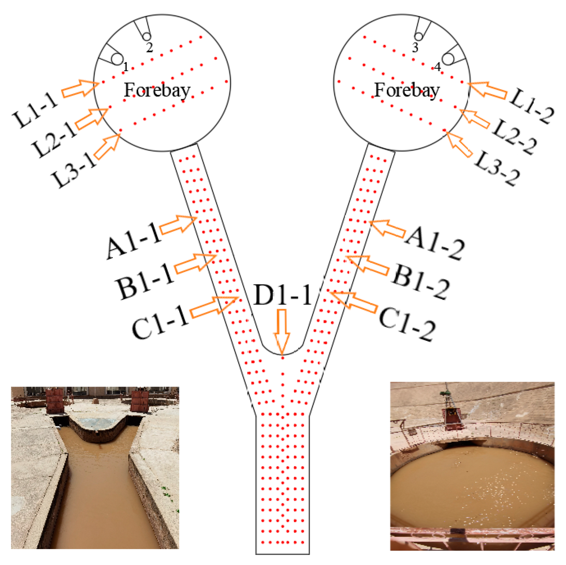
2.1. Research Area
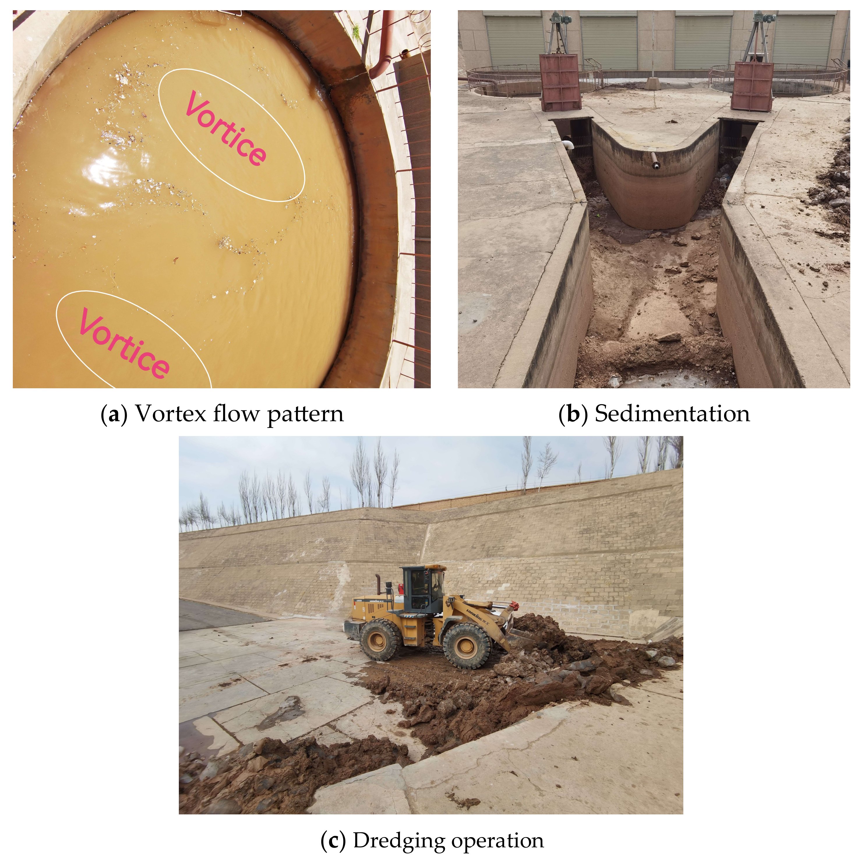
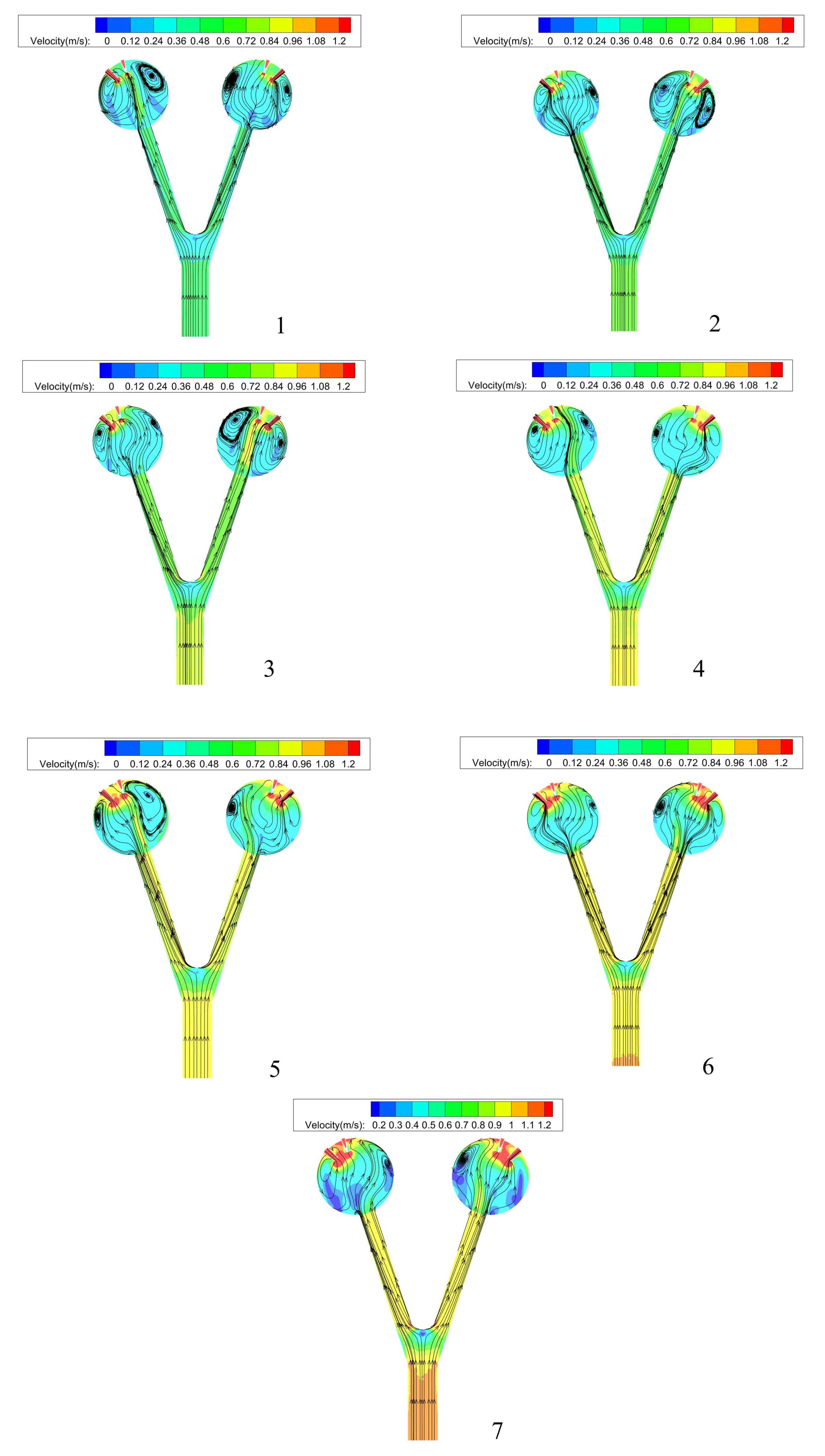
- Vortex formation and nonuniform flow: Within the circular forebays, fluid dynamics give rise to vortices and eddies. These intricate hydrodynamic phenomena can induce nonuniform flow profiles, notably affecting the inlet dynamics of the pump station and the operational efficacy of associated machinery.
- Sediment accumulation: Gansu Province’s geographical positioning within the middle and upper reaches of the Yellow River exposes it to a risk of heightened sediment content. This can lead to the ingress of considerable sediment loads from canal waters into circular forebays. In regions characterized by diminished flow velocities within circular forebays, sediment particulates tend to deposit along the substrate and sidewalls, leading to sedimentary deposition.
- Uneven horizontal distribution and flow velocity distribution: The prevailing heterogeneities in horizontal and flow velocity distributions indigenous to circular forebays have the potential to induce perturbations in inlet stability, leading to measurable reductions in pump station operational efficiency. These nonuniformities can be attributed to an intricate interplay of factors encompassing inlet flow rates, basin geomorphology, and sidewall configurations.
- Temporal fluctuations in water elevation and pressure gradients: The temporal oscillations in water elevation and concomitant pressure gradients within circular forebays have a pronounced influence on the operational modalities and inlet conditions of pumping stations. Misaligned water level dynamics and pressure gradients can present challenges ranging from flow instabilities to hydraulic perturbations.
2.2. Research Data and Calculation Methods
2.2.1. Research Data
2.2.2. Control Equation
- The mixture model [23] can proficiently capture the intricacies of solid-fluid coupling in water and sand two-phase flow within circular forebays. Accounting for interactions and mutual influences between the water and sand phases significantly enhances the precision of simulation outcomes.
- The mixture model [24] can seamlessly accommodate scenarios involving mixed water–sand flow within diversion channels, characterized by incompressible fluid dynamics. This adaptability ensures the fidelity and accuracy of simulations.
- The mixture model [25] demonstrates a credible alignment with the complexities of sediment distribution, vortex formation, and the behavior of low-load particles within circular forebays. It can adeptly consider factors such as momentum continuity, relative velocities, and volume fractions of distinct particles, thereby providing a more accurate portrayal of mixture motion characteristics.
- The algebraic expressions intrinsic to the mixture model can be effectively solved and simulated through numerical methodologies. This feature streamlines the computational process and facilitates the comprehensive analysis of dynamic attributes in water and sediment two-phase flow within circular forebays.
2.3. Reynolds Equation, Grid Division, and Boundary Conditions
2.3.1. Reynolds Equation
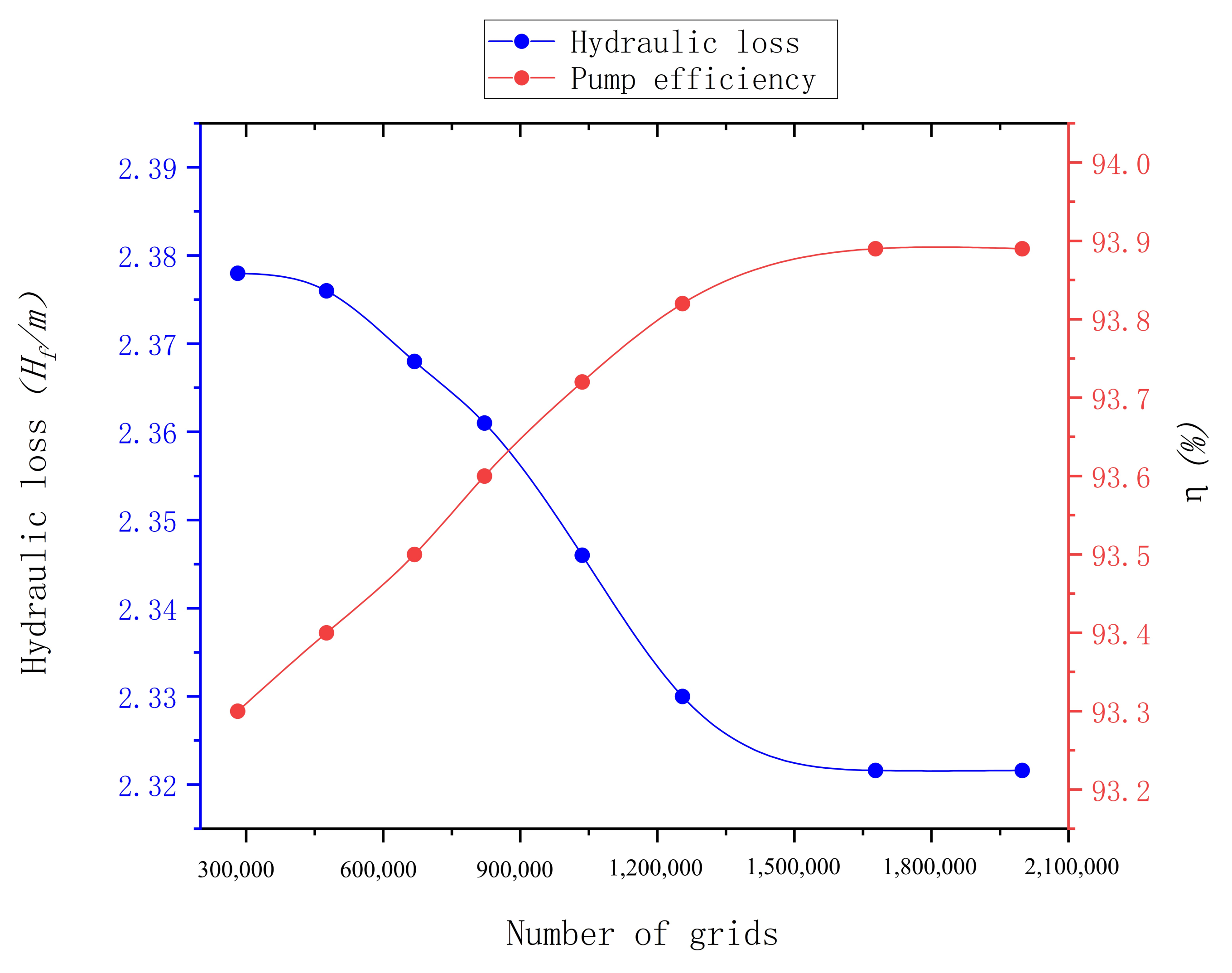
2.3.2. Mesh Generation
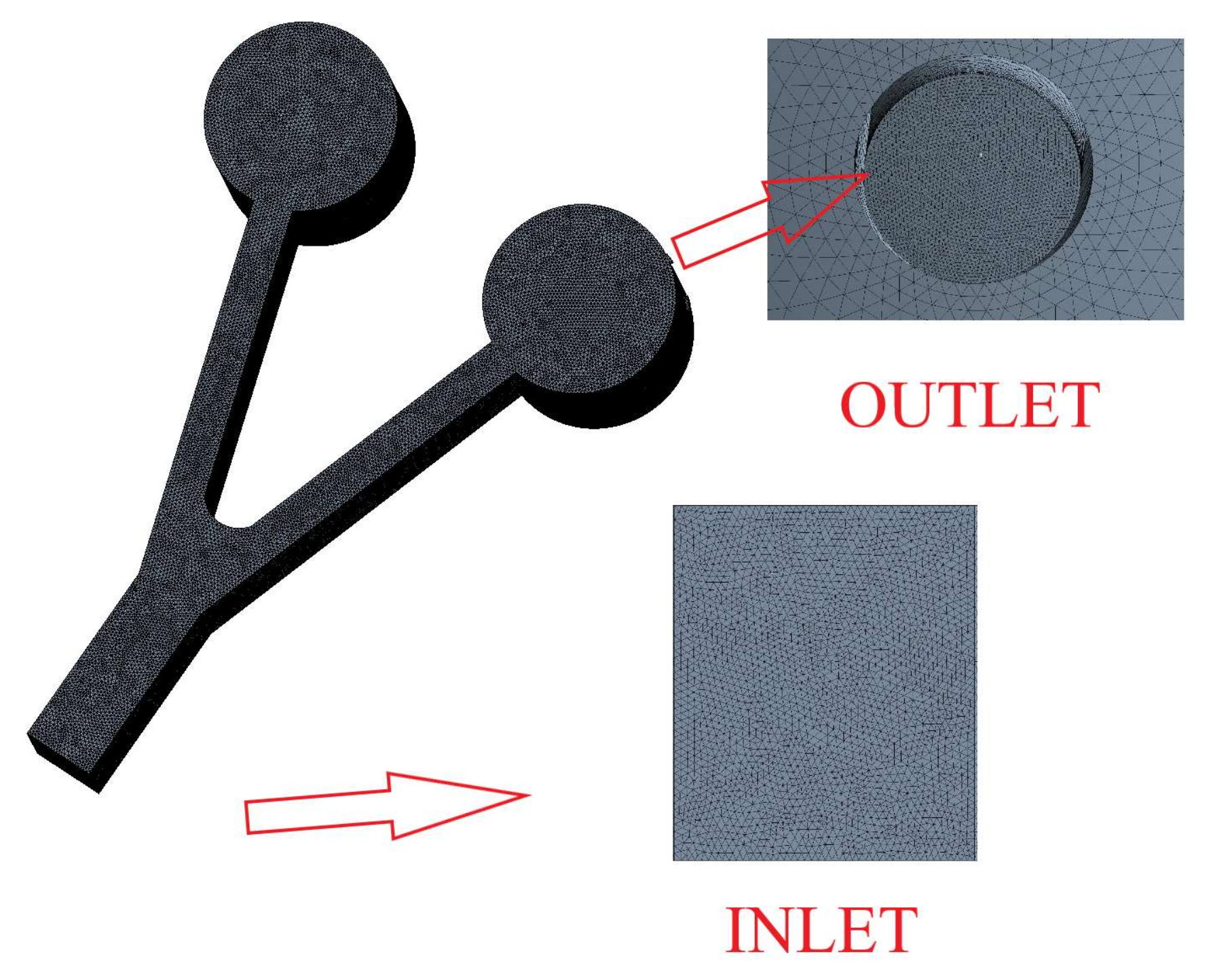
2.3.3. Boundary Conditions
3. Results
3.1. Working Condition Arrangement
3.1.1. Alterations in Flow Patterns among Various Schemes
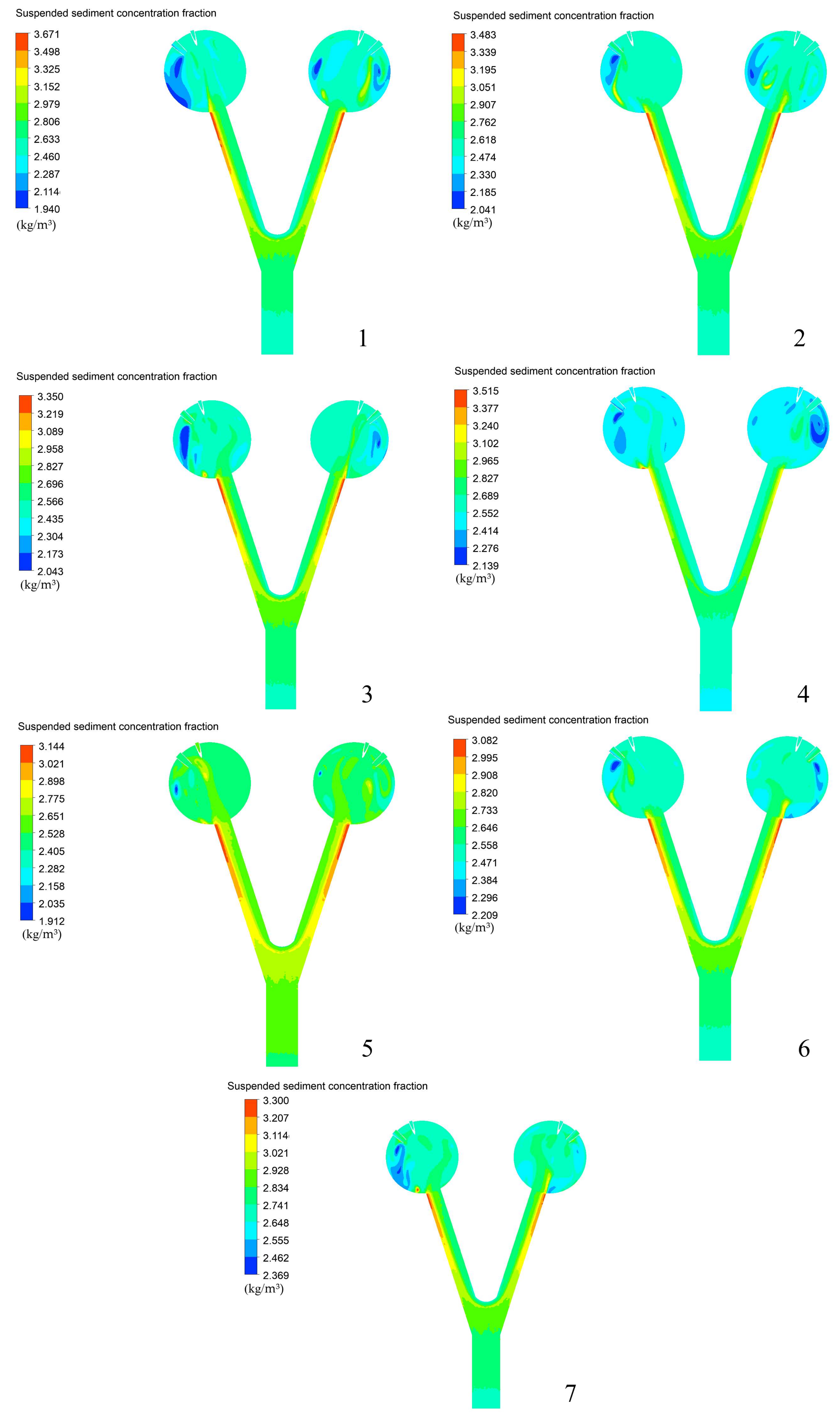
3.1.2. Alterations in Sediment Content among Various Schemes
3.2. Parameter Verification for Each Scheme
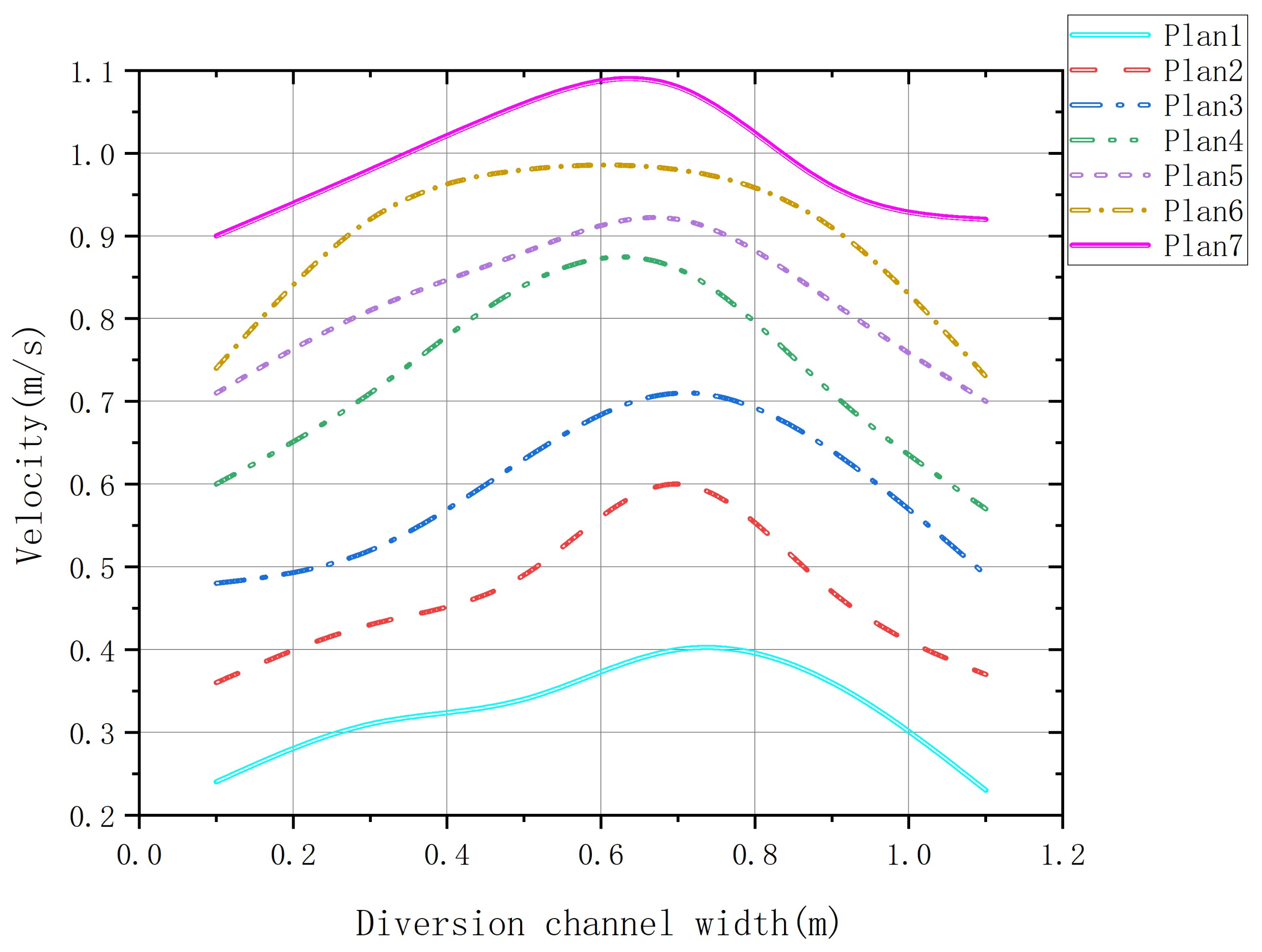
3.2.1. Flow Velocity, Uniformity, and Deviation Angle
3.2.2. Vortex Reduction Estimation
4. Discussion
4.1. Analysis of Flow Patterns in Different Schemes
4.2. Analysis of Sediment Content in Different Schemes
- Suspended Sediment: When encountering larger or unstable vortex flows, sediment in the water becomes suspended as a result of turbulence. These suspended particles tend to fluctuate with the movement of vortices. Higher vortex velocities hinder sediment settling in the bottom areas, decreasing the likelihood of sediment accumulation. In such cases, sediment is usually carried away with pumping action, although high sediment loads may lead to pump inlet blockage.
- Localized Sediment Deposition: Smaller and more stable vortex flows can lead to sediment deposition in specific areas, creating concentrated sediment accumulation zones. This situation is significantly influenced by flow velocity and patterns. For instance, even though there might not be vortex zones along the sidewalls, the flow speed of the mixed flow is lower than the sediment-carrying velocity. Consequently, sediment tends to accumulate extensively along the sidewalls of the Y-shaped diversion piers. This has a substantial impact on the main flow trajectory.
4.3. Integrated Analysis of the Optimal Scheme Based on Flow Velocity Uniformity, Deviation Angle, and Vortex Reduction Estimation
4.3.1. Analysis of Flow Velocity, Uniformity, and Deviation Angle
4.3.2. Analysis of the Vortex Reduction Area Parameter Ratio and Vortex Area Reduction Rate
4.4. Experimental Verification
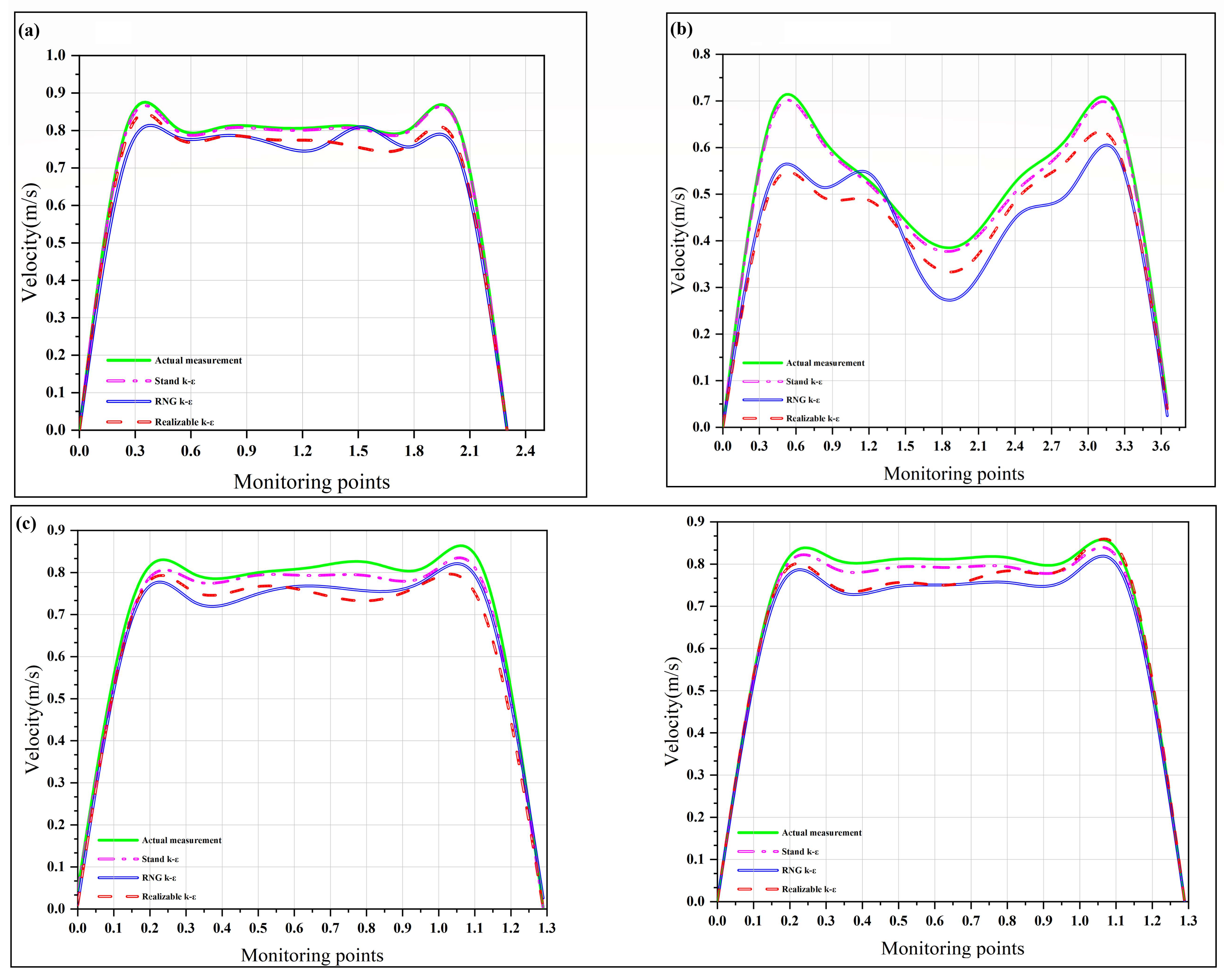
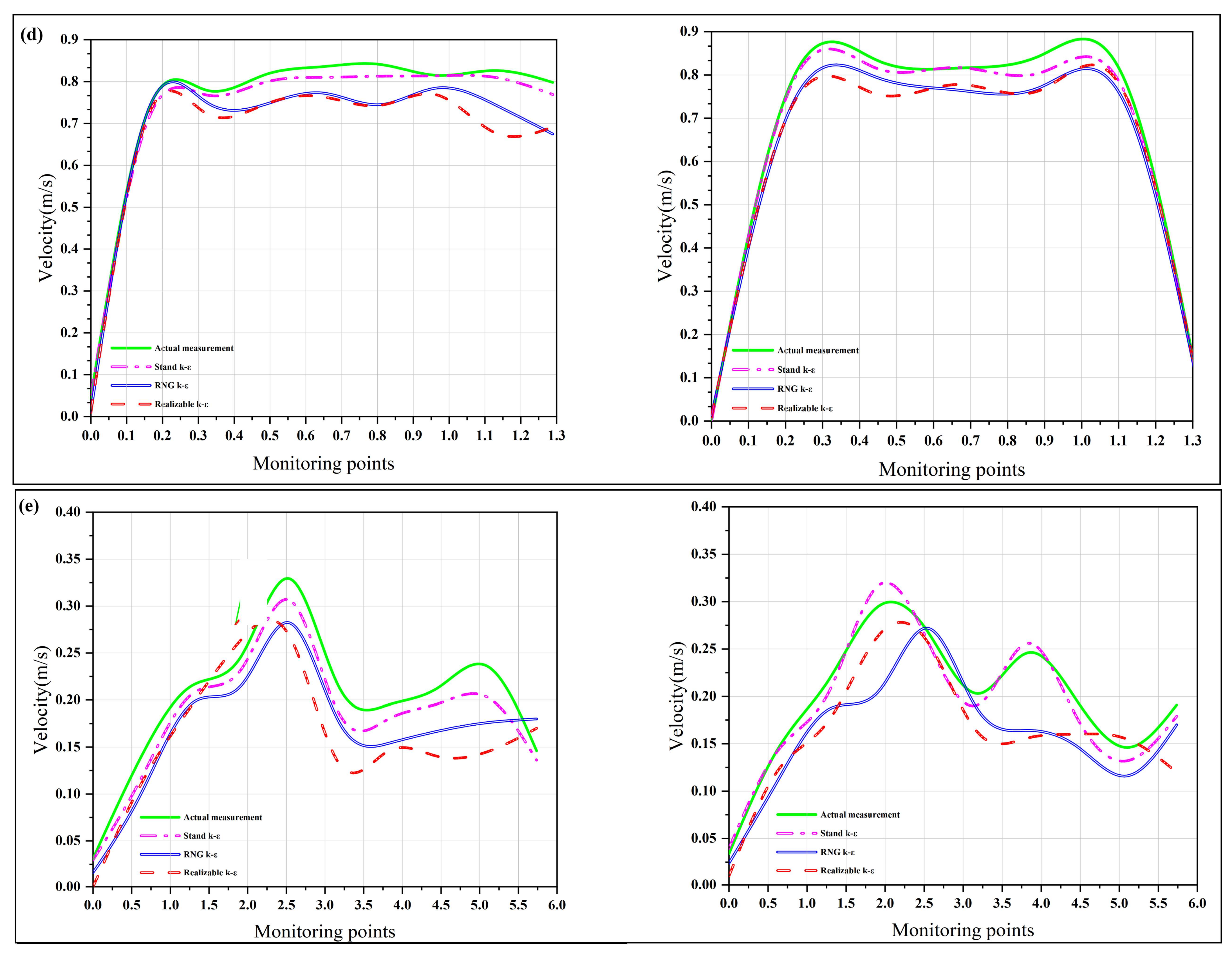
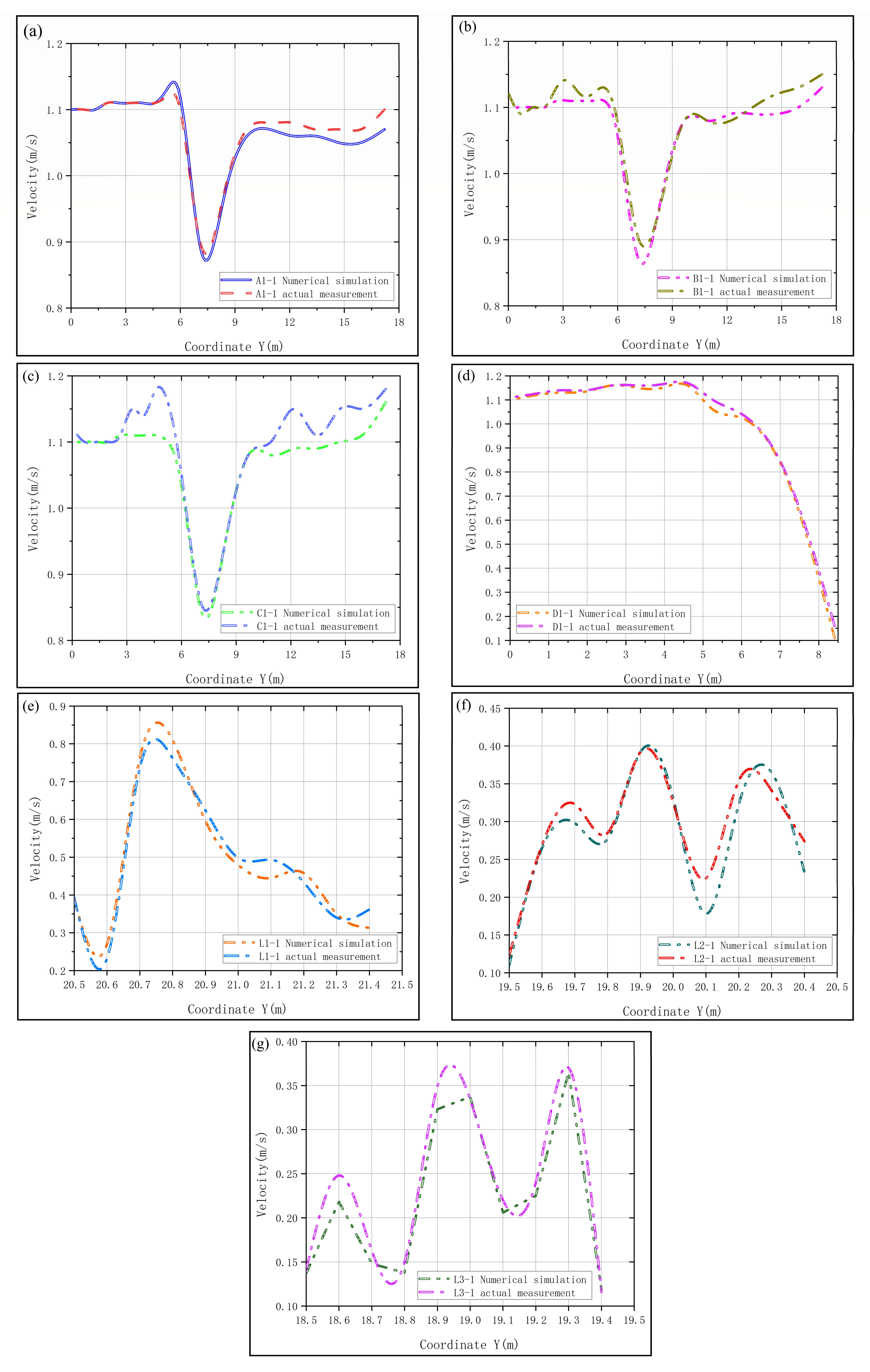
4.4.1. Flow Velocity Verification
4.4.2. Sediment Accumulation Verification
5. Conclusions
- (1)
- Using numerical simulation to calculate the flow patterns in different turbulence models and comparing the calculation results with multiple engineering measurements to confirm that the standard model conforms to actual operating conditions.
- (2)
- Through theoretical analysis of simulation results of different flow velocities of water and sediment two-phase flow, it can be concluded that the flow state of the diversion channel is relatively stable, but there will be obvious vortices generated in the forebay, and there will be varying degrees of sediment accumulation in the diversion channel and forebay.
- (3)
- The flow pattern in the forebay will change to varying degrees with the flow velocity. From Scheme 1 to Scheme 6, as the flow velocity increases, the optimization performance of the flow pattern gradually improves, and the sediment content also shows a decreasing state. However, when the flow velocity is increased again in Scheme 7, the flow pattern further deteriorates, and the sediment content also increases.
- (4)
- At the initial flow rate of Scheme 6, the uniformity of the flow rate is improved by 4.82% compared to Scheme 1, and the deviation angle is reduced by 4.69°. The parameter ratio of the vortex reduction area and the reduction rate of the vortex area have been significantly optimized. Therefore, condition 6 is the optimal initial flow rate.
- (5)
- After adopting Scheme 6 for operation in the project, the actual flow velocity in the forebay was basically consistent with the numerical simulation results. The sediment deposition had a significant reduction effect compared to the previous year, and the sediment deposition thickness was reduced to its maximum extent by 0.67 m.
Author Contributions
Funding
Data Availability Statement
Conflicts of Interest
References
- Yonghai, Y.; Haodi, Y.; Changliang, Y. Parameter optimization of rectification sill in the forebay of pumping station using BPNN-GA algorithm. Trans. Chin. Soc. Agric. Eng. 2023, 39, 106–113. [Google Scholar]
- Zhang, Y. Study on Hydraulic Characteristics of Forebay and Sump of Large Pumping Station. Master’s Thesis, Xi’an University of Technology, Xi’an, China, 2022. (In Chinese). [Google Scholar]
- Xinjian, F.; Chunhai, D.; Zhijun, W.; Ya’Nan, L.; Wei, Y. Influence of diffusion angle on flow field structure in forward intake forebay of pumping station. Trans. Chin. Soc. Agric. Eng. 2023, 39, 92–99. [Google Scholar]
- Ming, L.; Yong, W.; Wei, X.; Xiaolin, W.; Houlin, L. Optimizing the geometric parameters for the lateral inflow forebay of the pump sump. Trans. Chin. Soc. Agric. Eng. 2022, 38, 69–77. [Google Scholar]
- Zhang, C.; Yan, H.; Jamil, M.T.; Yu, Y. Improvement of the Flow Pattern of a Forebay with a Side-Intake Pumping Station by Diversion Piers Based on Orthogonal Test Method. Water 2022, 14, 2663. [Google Scholar] [CrossRef]
- Wang, H.; Li, C.; Lu, S.; Song, L. The flow patterns and sediment deposition in the forebay of a forward-intake pumping station. Phys. Fluids 2022, 34, 083316. [Google Scholar] [CrossRef]
- Fujun, W.; Xuelin, T.; Xin, C.; Ruofu, X.; Zhifeng, Y.; Wei, Y. A review on flow analysis method for pumping stations. J. Hydraul. Eng. 2018, 49, 47–61. [Google Scholar]
- Li, Y.; Gu, J.; Guo, C.; Zhou, C. Flow Patterns and Rectification Measures in the Forebay of Pumping Station. IOP Conf. Ser. Mater. Sci. Eng. 2020, 794, 12058. [Google Scholar] [CrossRef]
- Zhan, J.M.; Wang, B.C.; Yu, L.H.; Li, Y.S.; Ling, T. Numerical investigation of flow patterns in different pump intake systems. J. Hydrodyn. 2012, 24, 873–882. [Google Scholar] [CrossRef]
- Hui, F.; Huasi, N.; Yujia, M.; Ruobing, Y.; Xinlei, G.; Chunrong, S. Hydraulic performance optimization of the ultra narrow union pumping forebay: A case study. J. Hydraul. Eng. 2020, 51, 788–795. [Google Scholar]
- Can, L.; Shuaihao, L.; Yao, Y.; Li, C.; Du, K. Numerical simulation research on inlet flow pattern of small sluice station lateral pumping station. J. Drain. Irrig. Mach. Eng. 2021, 39, 797–803. [Google Scholar]
- Xu, C.; Wang, R.; Liu, H.; Zhang, R.; Wang, M.; Wang, Y. Flow pattern and anti-silt measures of straight-edge forebay in large pump stations. Int. J. Heat Technol. 2018, 36, 1130–1139. [Google Scholar] [CrossRef]
- Caishui, H. Three-dimensional Numerical Analysis of Flow Pattern in Pressure Forebay of Hydropower Station. Procedia Eng. 2012, 28, 128–135. [Google Scholar] [CrossRef]
- Nasr, A.; Yang, F.; Zhang, Y.; Wang, T.; Hassan, M. Analysis of the Flow Pattern and Flow Rectification Measures of the Side-Intake Forebay in a Multi-Unit Pumping Station. Water 2021, 13, 2025. [Google Scholar] [CrossRef]
- Xi, W.; Lu, W.G. Formation Mechanism of an Adherent Vortex in the Side Pump Sump of a Pumping Station. Int. J. Simul. Model. 2021, 20, 327–338. [Google Scholar] [CrossRef]
- Tang, X.; Wang, W.; Wang, F.; Yu, X.; Chen, Z.; Shi, X. Application of LBM-SGS Model to Flows in a Pumping-Station Forebay. J. Hydrodyn. 2010, 22, 196–206. [Google Scholar] [CrossRef]
- Xu, W.; Cheng, L.; Du, K.; Yu, L.; Ge, Y.; Zhang, J. Numerical and Experimental Research on Rectification Measures for a Contraction Diversion Pier in a Pumping Station. J. Mar. Sci. Eng. 2022, 10, 1437. [Google Scholar] [CrossRef]
- Lyons, M.; Simmons, S.; Fisher, M.; Williams, J.S.; Lubitz, W.D. Experimental Investigation of Archimedes Screw Pump. J. Hydraul. Eng. 2020, 146, 4020057. [Google Scholar] [CrossRef]
- Parsons, A.J.; Bracken, L.; Poeppl, R.E.; Wainwright, J.; Keesstra, S.D. Introduction to special issue on connectivity in water and sediment dynamics. Earth Surf. Proc. Land 2015, 40, 1275–1277. [Google Scholar] [CrossRef]
- Budinski, L.; Spasojević, M. 2D Modeling of Flow and Sediment Interaction: Sediment Mixtures. J. Waterw. Port Coast. Ocean Eng. 2014, 140, 199–209. [Google Scholar] [CrossRef]
- Serra, T.; Soler, M.; Barcelona, A.; Colomer, J. Suspended sediment transport and deposition in sediment-replenished artificial floods in Mediterranean rivers. J. Hydrol. 2022, 609, 127756. [Google Scholar] [CrossRef]
- Yuan, Q.; Zhang, M.; Zhou, J. To Implement A Clear-Water Supply System for Fine-Sediment Experiment in Laboratories. Water 2019, 11, 2476. [Google Scholar] [CrossRef]
- Mirmasoumi, S.; Behzadmehr, A. Numerical study of laminar mixed convection of a nanofluid in a horizontal tube using two-phase mixture model. Appl. Therm. Eng. 2008, 28, 717–727. [Google Scholar] [CrossRef]
- Li, J.N.; Chen, X.H. A multi-dimensional two-phase mixture model for intense sediment transport in sheet flow and around pipeline. Phys. Fluids 2022, 34, 103314. [Google Scholar] [CrossRef]
- Onishi, T.; Peng, Y.; Ji, H.; Peng, G. Numerical simulations of cavitating water jet by an improved cavitation model of compressible mixture flow with an emphasis on phase change effects. Phys. Fluids 2023, 35, 73333. [Google Scholar] [CrossRef]
- Almeland, S.K.; Olsen, N.R.B.; Bråveit, K.; Aryal, P.R. Multiple solutions of the Navier-Stokes equations computing water flow in sand traps. Eng. Appl. Comp. Fluid 2019, 13, 199–219. [Google Scholar] [CrossRef]
- Ozmen-Cagatay, H.; Kocaman, S. Dam-Break Flow in the Presence of Obstacle: Experiment and CFD Simulation. Eng. Appl. Comp. Fluid 2011, 5, 541–552. [Google Scholar] [CrossRef]
- Ghai, S.K.; Ahmed, U.; Klein, M.; Chakraborty, N. Turbulent kinetic energy evolution in turbulent boundary layers during head-on interaction of premixed flames with inert walls for different thermal boundary conditions. Proc. Combust. Inst. 2023, 39, 2169–2178. [Google Scholar] [CrossRef]
- Zhao, L.; Liu, D.; Lin, J.; Chen, L.; Chen, S.; Wang, G. Estimation of turbulent dissipation rates and its implications for the particle-bubble interactions in flotation. Miner. Eng. 2023, 201, 108230. [Google Scholar] [CrossRef]
- Cheng, Y.; Lien, F.S.; Yee, E.; Sinclair, R. A comparison of large Eddy simulations with a standard k–ε Reynolds-averaged Navier–Stokes model for the prediction of a fully developed turbulent flow over a matrix of cubes. J. Wind. Eng. Ind. Aerodyn. 2003, 91, 1301–1328. [Google Scholar] [CrossRef]
- Ahn, S.; Xiao, Y.; Wang, Z.; Luo, Y.; Fan, H. Unsteady prediction of cavitating flow around a three dimensional hydrofoil by using a modified RNG k-ε model. Ocean Eng. 2018, 158, 275–285. [Google Scholar] [CrossRef]
- Moen, A.; Mauri, L.; Narasimhamurthy, V.D. Comparison of k-ε models in gaseous release and dispersion simulations using the CFD code FLACS. Process. Saf. Environ. 2019, 130, 306–316. [Google Scholar] [CrossRef]
- Oosterkamp, A.; Ytrehus, T.; Galtung, S.T. Effect of the choice of boundary conditions on modelling ambient to soil heat transfer near a buried pipeline. Appl. Therm. Eng. 2016, 100, 367–377. [Google Scholar] [CrossRef]
- Folkner, D.; Katz, A.; Sankaran, V. Design and verification methodology of boundary conditions for finite volume schemes. Comput. Fluids 2014, 96, 264–275. [Google Scholar] [CrossRef]
- Sojoudi, A.; Nourbakhsh, A.; Shokouhmand, H. Establishing a Relationship between Hydraulic Efficiency and Temperature Rise in Centrifugal Pumps: Experimental Study. J. Hydraul. Eng. 2018, 144, 4018011. [Google Scholar] [CrossRef]
- Hadžiabdić, M.; Ničeno, B. Reconstruction of Nusselt number in RANS computations with wall function approach. Nucl. Eng. Des. 2023, 412, 112461. [Google Scholar] [CrossRef]
- Wang, H.; Li, C.; Lu, S.; Yang, C.; Huang, L. Numerical and experimental study on vortex optimization in the forebay of a Sandy River. Phys. Fluids 2023, 35, 085128. [Google Scholar] [CrossRef]
- Zi, D.; Wang, F.; Yao, Z.; Hou, Y.; Xiao, R.; He, C.; Yang, E. Effects analysis on rectifying intake flow field for large scale pumping station with combined diversion piers. Trans. Chin. Soc. Agric. Eng. 2015, 31, 71–77. [Google Scholar]
- Yang, F.; Zhang, Y.; Liu, C.; Wang, T.; Jiang, D.; Jin, Y. Numerical and Experimental Investigations of Flow Pattern and Anti-Vortex Measures of Forebay in a Multi-Unit Pumping Station. Water 2021, 13, 935. [Google Scholar] [CrossRef]


| Project | Month | Annual | |||||||||||
|---|---|---|---|---|---|---|---|---|---|---|---|---|---|
| 1 | 2 | 3 | 4 | 5 | 6 | 7 | 8 | 9 | 10 | 11 | 12 | ||
| Water volume (B m3) | 1.62 | 1.651 | 1.726 | 1.899 | 1.912 | 2.098 | 2.152 | 2.998 | 3.102 | 2.935 | 1.536 | 1.498 | 25.127 |
| Sediment (M kg) | 48.15 | 37.42 | 158.63 | 392.41 | 1149.56 | 1432.12 | 4563.32 | 11,204.13 | 5736.45 | 8213.65 | 283.61 | 145.56 | 33,365.01 |
| Sediment concentration (kg/m3) | 0.029 | 0.023 | 0.092 | 0.207 | 0.601 | 0.683 | 2.121 | 3.737 | 1.849 | 2.799 | 0.185 | 0.097 | 1.328 |
| Schemes | Inlet Flow ) | Inlet Velocity ) |
|---|---|---|
| 1 | 3.39 | 0.6 |
| 2 | 3.955 | 0.7 |
| 3 | 4.52 | 0.8 |
| 4 | 5.085 | 0.9 |
| 5 | 5.65 | 1.0 |
| 6 | 6.215 | 1.1 |
| 7 | 6.78 | 1.2 |
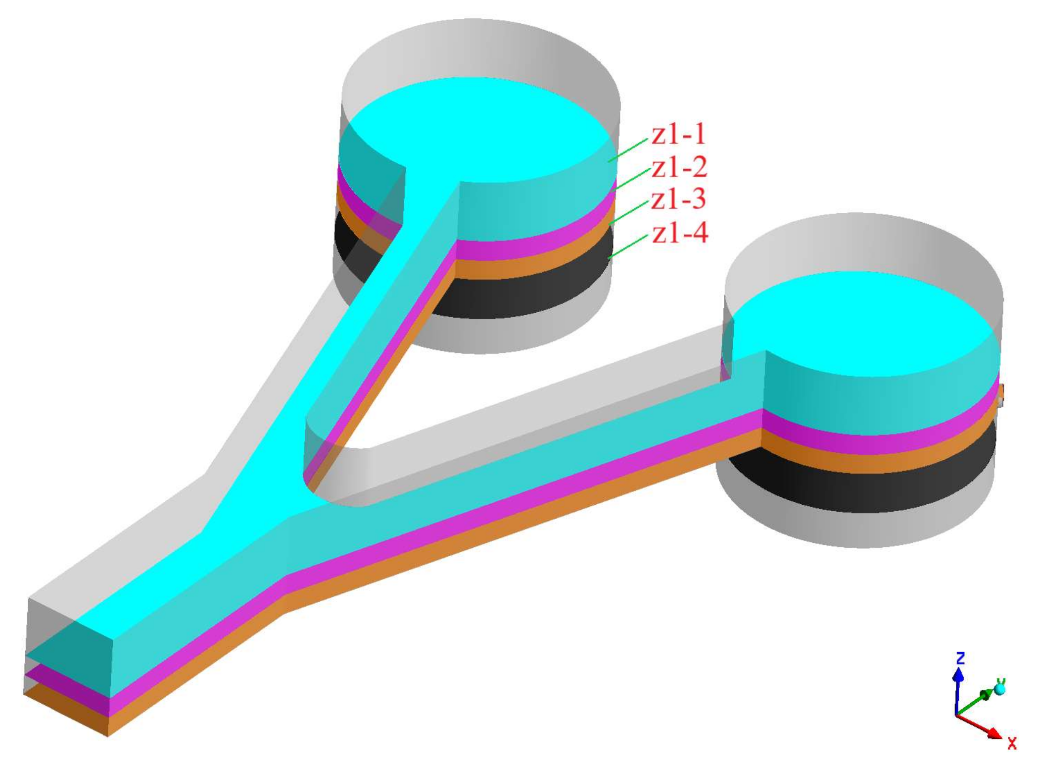
| Section | Section Position |
|---|---|
| z1−1 | |
| z1−2 | |
| z1−3 | |
| z1−4 |
| Different Phases | Viscosities () | Densities () | Volume Fraction Ratio () | Time |
|---|---|---|---|---|
| Water | 0.001 | 1000 | 99.8952 | 110 days |
| Sand | 0.000103 | 2500 | 0.1048 | 110 days |
| Schemes | Observation Sections | ||
|---|---|---|---|
| 1 | 84.63 | 20.12 | |
| 2 | 85.89 | 19.87 | |
| 3 | 86.15 | 18.94 | |
| 4 | 87.22 | 17.56 | |
| 5 | 87.68 | 16.81 | |
| 6 | 89.45 | 15.43 | |
| 7 | 87.31 | 16.95 |
| Schemes | Vortex Area | Circular Forebay Area | Vortex Area Parameter Ratio (%) | Reduction Rate (%) |
|---|---|---|---|---|
| 1 | 19.815 | 26.421 | 74.99 | - |
| 2 | 19.031 | 26.421 | 72.03 | 3.96 |
| 3 | 17.967 | 26.421 | 68.01 | 9.33 |
| 4 | 16.586 | 26.421 | 62.78 | 16.30 |
| 5 | 15.421 | 26.421 | 58.37 | 22.18 |
| 6 | 12.352 | 26.421 | 46.75 | 37.66 |
| 7 | 15.953 | 26.421 | 60.38 | 19.49 |
Disclaimer/Publisher’s Note: The statements, opinions and data contained in all publications are solely those of the individual author(s) and contributor(s) and not of MDPI and/or the editor(s). MDPI and/or the editor(s) disclaim responsibility for any injury to people or property resulting from any ideas, methods, instructions or products referred to in the content. |
© 2023 by the authors. Licensee MDPI, Basel, Switzerland. This article is an open access article distributed under the terms and conditions of the Creative Commons Attribution (CC BY) license (https://creativecommons.org/licenses/by/4.0/).
Share and Cite
Wang, H.; Tai, Y.; Huang, L.; Yang, C.; Jing, H. Analyzing Water and Sediment Flow Patterns in Circular Forebays of Sediment-Laden Rivers. Sustainability 2023, 15, 16941. https://doi.org/10.3390/su152416941
Wang H, Tai Y, Huang L, Yang C, Jing H. Analyzing Water and Sediment Flow Patterns in Circular Forebays of Sediment-Laden Rivers. Sustainability. 2023; 15(24):16941. https://doi.org/10.3390/su152416941
Chicago/Turabian StyleWang, Haidong, Yuji Tai, Lingxiao Huang, Cheng Yang, and Hefang Jing. 2023. "Analyzing Water and Sediment Flow Patterns in Circular Forebays of Sediment-Laden Rivers" Sustainability 15, no. 24: 16941. https://doi.org/10.3390/su152416941
APA StyleWang, H., Tai, Y., Huang, L., Yang, C., & Jing, H. (2023). Analyzing Water and Sediment Flow Patterns in Circular Forebays of Sediment-Laden Rivers. Sustainability, 15(24), 16941. https://doi.org/10.3390/su152416941