Performance Analysis and Multi-Objective Optimization of a Cooling-Power-Desalination Combined Cycle for Shipboard Diesel Exhaust Heat Recovery

Abstract

This study presents a novel cooling-power-desalination combined cycle for recovering shipboard diesel exhaust heat, integrating a freezing desalination sub-cycle to regulate the ship’s cooling-load fluctuations. The combined cycle employs ammonia–water as the working fluid and efficiently utilizes excess cooling capacity to pretreat reverse osmosis desalination. By adjusting the mass flow rate of the working fluid in both the air conditioning refrigeration cycle and the freezing desalination sub-cycle, the combined cycle can dynamically meet the cooling-load demand under different working conditions and navigation areas. To analyze the cycle’s performance, a mathematical model is established for energy and exergy analysis, and key parameters including net output work, comprehensive efficiency, and heat exchanger area are optimized using the MOPSO algorithm. The results indicate that the system achieves optimal performance when the generator temperature reaches 249.95 °C, the sea water temperature is 22.29 °C, and 42% ammonia–water is used as the working fluid. Additionally, an economic analysis of frozen seawater desalination as RO seawater desalination pretreatment reveals a substantial cost reduction of 22.69%, showcasing the advantageous features of this proposed cycle. The research in this paper is helpful for waste energy recovery and sustainable development.

1. Introduction

Shipping has consistently remained the most economical mode of transportation, fulfilling 90% of the world’s transportation requirements [1]. Due to stringent emission laws [2,3], energy shortages, and the pressing concerns of global warming, the significance of energy conservation and environmental protection has intensified. Consequently, the recycling of waste heat from ships emerges as a pivotal approach to energy preservation. Throughout a ship’s journey, the diesel engine, serving as the primary power unit, expels a substantial amount of heat through jacket water and exhaust gas. This waste heat, categorized as low-grade energy, can be efficiently reclaimed through the thermodynamic cycle.

Currently, in this stage of research, the thermodynamic cycle is predominantly employed to convert low- and medium-grade heat energy into electrical energy for recycling purposes. Song [4] et al. recovered waste heat from exhaust gas and jacket water through organic Rankine cycle (ORC), comprehensively considered thermal performance, system structure and economic feasibility, compared various different ORC systems, and carried out thermodynamic analysis and system performance optimization. Yang [5,6,7] studied the performance of the transcritical ORC in recycling diesel engine waste heat, and analyzed the performance and economic analysis of three different waste heat recovery models and six different organic working fluids. Mat Nawi [8] et al. studied the effects of mass flow and temperature difference on ORC results, and proposed to use bioethanol produced by synechococcus PCC 7002 as a clean energy source for circular working fluids. Feng [9] et al. proposed that the Brayton–Kalina combined cycle system using supercritical carbon dioxide as the circulating working fluid recovers the waste heat of the low-speed diesel engine, which makes full use of the waste heat of the ship’s diesel engine and reduces the energy efficiency design index of the system. Sakalis [10] studied the waste heat recovery potential of supercritical carbon dioxide as a working medium, studied the waste heat recovery at three different temperature levels: exhaust gas, compressed scavenge air, and jacket cooling water, and improved the energy efficiency of the cycle. Gürgen [11] et al. took a container ship with a capacity of 2200 TEU as an example, comprehensively considered the thermodynamic properties, economy, safety and environmental standards of 10 different working fluids, and adopted the Multi-Objective Gray Wolf algorithm to study the performance of organic Rankine cycles.

In the research discussed above, the ongoing challenges in ship waste heat cycles persist. The demand for electricity frequently coincides with the demand for refrigeration during voyages, and challenges persist within the current ship waste heat cycle. During ship voyages, the need for electricity is often coupled with the requirement for refrigeration. Under typical conditions, the waste heat from the exhaust gas is converted into electrical energy, which is then utilized for ice production to fulfill the cooling demand [12,13]. Nevertheless, the secondary energy conversion involved in this electricity-based refrigeration production method gives rise to energy losses that cannot be overlooked. Enhancing the energy utilization-rate of waste heat from ship exhaust and achieving the dual objectives of electricity and refrigeration have emerged as pressing concerns in this domain. It is noteworthy that, similar to thermoelectric systems, the waste heat-driven combined power and refrigeration cycle is considered highly efficient, capable of generating both power and refrigeration in a single thermodynamic cycle [14,15,16,17]. Nonetheless, the combined power and refrigeration cycle encounters a significant issue when applied to ships. The flue gas temperature of a ship’s main engine varies with operating conditions, leading to substantial fluctuations [18]. Simultaneously, the ship’s air conditioning experiences considerable cooling-load variations throughout the day [19,20]. The aforementioned issues can be summarized as fluctuations in the input energy-output load of the thermodynamic cycle and the instability of the operating environment of the thermodynamic cycle. Consequently, if the combined power and refrigeration cycle were directly employed for waste heat utilization on the ship, it would frequently operate outside the designated parameters, significantly impairing the comprehensive efficiency of heat energy circulation. This constitutes the main challenge addressed in the present investigation.

To address the aforementioned issues, this paper introduces seawater desalination technology [21,22,23] into the combined power and refrigeration cycle, proposing a novel marine diesel exhaust heat-driven ammonia–water absorption cooling-power-desalination combined cycle (CPDCC). Firstly, to address fluctuations in refrigeration demand, this paper introduces a novel approach: utilizing excess cooling capacity for seawater icing to fulfill the ship’s cooling-load requirements and enhancing system stability through seawater desalination. Secondly, in response to varying ship working conditions, this paper analyzes the thermal cycle’s performance under diverse operating scenarios. A single thermal cycle can concurrently generate power, provide refrigeration, support cold storage, facilitate desalination, and deliver other outputs, significantly enhancing the overall utilization efficiency of marine exhaust heat energy. Thirdly, among existing desalination methods, frozen-seawater desalination yields low efficiency but low cost, while RO desalination is efficient but expensive [24,25,26,27]. Consequently, this study integrates the strengths of both methods, utilizing seawater-freezing desalination to significantly lower the feedwater salinity for reverse osmosis desalination, thereby reducing overall seawater desalination costs.

However, there is limited research focused on thermal cycle systems designed to address the variability in diesel exhaust gas and the fluctuations in ship cooling-load demand. The research conducted in this paper aims to solve the existing problems in diesel exhaust waste heat recovery due to the fluctuation in working conditions and cooling-load demand. This paper presents a CPDCC system capable of adjusting cooling capacity-output direction. The primary aim of this study is to enhance the thermal design basis of the CPDCC by optimizing its performance under varying heat source temperatures, cooling loads, and diverse sea conditions. To achieve this, the distinction between cooling energy and electrical energy grades was considered, and a comprehensive evaluation of system efficiency was performed using exergy analysis. A thorough variable working condition analysis was conducted, taking into account the variations in sea temperatures across different regions and timeframes, as well as the impact of diverse concentrations of the working fluid on the overall performance of the CPDCC. As decision variables, appropriate ranges for generation and condensation temperatures, mass fraction of ammonia, and reflux ratio were carefully selected. To find the best possible solutions, the Multi-Objective Particle Swarm Optimization (MOPSO) algorithm was applied. The optimization objectives were aimed at improving the net output work, cycle comprehensive efficiency, and heat exchanger area. By utilizing the MOPSO algorithm, a set of Pareto optimal solutions was sought. From the set of Pareto optimal solutions, the Technique for Order of Preference by Similarity to Ideal Solution (TOPSIS) decision method was employed to identify the most suitable and efficient solution. Valuable insights into the optimal design and operation of the CPDCC under various conditions are provided by this final Pareto optimal solution, enabling better performance and resource management. Moreover, to address onboard seawater desalination challenges, the cycle cooling capacity produced by the CPDCC serves for secondary freezing desalination of seawater and acts as pretreatment for RO desalination. During the freezing desalination pretreatment, the cold volume resulting from sea ice melting can also be additionally reclaimed. Within this investigation, the economic aspects of this desalination process were scrutinized and a cost comparison was performed against RO desalination that lacks freezing pretreatment.

2. Materials and Methods

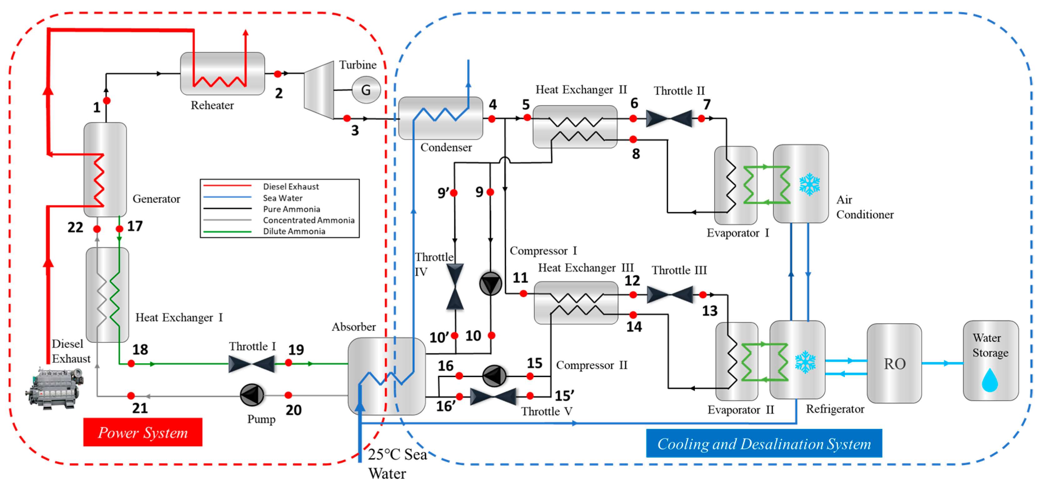
2.1. Cycle Operating Principle

Figure 1 shows a schematic of the cooling-power-desalination combined cycle (CPDCC). In the CPDCC, dilute ammonia–water (22) is fed into the generator and undergoes rectification to produce pure ammonia (1) and concentrated ammonia–water (17). The high-temperature and high-pressure vapor generated as pure ammonia passes through the reheater (2) and drives the rotation of the turbine to perform external work. The exhaust gas from the turbine (3) is directed into the seawater-cooled condenser, where it undergoes condensation to form saturated liquid ammonia (4). The exhaust gas from the turbine (3) is directed into the seawater-cooled condenser, where it undergoes condensation to form saturated liquid ammonia (4). After flow control, the saturated ammonia (4) enters both the air conditioning refrigeration cycle (5) and the cold storage desalination cycle (11). The low-temperature working fluid discharged from the heat exchanger and the evaporator undergoes heat exchange (6, 12) with the condensed ammonia. Subsequently, it is throttled through the throttle valve to the evaporator pressure (7, 13). Upon entering the evaporator, it undergoes the evaporation phase (8, 14) and transforms into saturated ammonia vapor. The heat absorbed during this process can meet the cooling capacity requirements of both the air conditioner and the cold storage. Subsequently, the saturated ammonia vapor is transferred by the heat exchanger (9, 15). The absorber pressure varies due to the different concentrations of ammonia–water. It is either throttled through the throttle valve or boosted to the absorber pressure (10, 16) by the compressor before entering the absorber. The high-temperature concentrated ammonia–water (17), flowing out of the generator, undergoes heat exchange with the low-temperature dilute ammonia–water (21) in heat exchanger I. Following throttling through the throttle valve I to the absorber pressure (19), it enters the absorber, where it combines with pure ammonia to form saturated dilute ammonia–water (20). Subsequently, the saturated dilute ammonia–water (20) is compressed by the working fluid pump (21), and after increasing the temperature (22) through heat exchange it is sent back to the generator for next cycle.

2.2. Mathematical Model

2.2.1. Mathematical Model Analysis

The cycle model was developed using the MATLAB R2021a framework, which facilitates the computation of mass and energy conversion processes within the cycle. The physical parameters of the recycled working fluid are obtained from the National Institute of Standards and Technology (NIST) database, and the REFPROP 9.0 physical property software, developed by NIST, is utilized for the calculation of state points.

During the cycle, the working fluid obeys the continuity equation. Specifically, the ammonia–water mixture must adhere to the mass conservation equation at every state point.

$${\Delta }_{out}^{in}\sum m_i=0$$

(1)

$${\Delta }_{out}^{in}\sum X_i{m}_i=0$$

(2)

where $m_i$ means the mass flow of the working fluids at each state points, and $X_i$ means the mass fraction of each component in the working fluids.

The thermodynamic performance analysis of the cycle’s state points is based on the equations. Within the generator, rectification of the concentrated ammonia–water yields dilute ammonia–water and pure ammonia. The heat absorbed during this process can be calculated as:

$$Q_{gen}=m_{17}{h}_{17}+m_1{h}_1-m_{22}{h}_{22}$$

(3)

The heat absorbed in the reheater can be calculated as:

$$Q_{re}=m_2{h}_2-m_1{h}_1$$

(4)

In the turbine, the high-temperature and -pressure vapors enter the expander to drive the rotation of the turbine and do external work, and the power output of turbine is calculated as:

$$W_{tur}=m_2{h}_2-m_3{h}_3=\left(m_2{h}_2-m_3{h}_{3s}\right){\eta }_t$$

(5)

where ${\eta }_t$ is the isentropic efficiency of turbine and $h_{3s}$ is specific enthalpy of working fluid at turbine inlet.

In the condenser, the exhaust gas discharged from the turbine enters and undergoes condensation, transforming into a saturated liquid state due to the cooling effect of circulating water. The released heat from the working fluids can be calculated as follows:

$$Q_{con}=m_3{h}_3-m_4{h}_4$$

(6)

In evaporator I and II, the liquid working fluid undergoes a phase transition and evaporates into a gaseous state, absorbing external heat. The absorbed heat is calculated as follows:

$$Q_{eva,I}=m_8{h}_8-m_7{h}_7$$

(7)

$$Q_{eva,II}=m_{14}{h}_{14}-m_{13}{h}_{13}$$

(8)

In the absorber, dilute ammonia–water is mixed with pure ammonia, releasing heat. The released heat is calculated as follows:

$$Q_{abs}=m_{10}{h}_{10}+m_{16}{h}_{16}+m_{19}{h}_{19}-m_{20}{h}_{20}$$

(9)

In the pump, the work performed by the pump on the fluid is calculated as:

$$W_{pump}=m_{21}{h}_{21}-m_{20}{h}_{20}=\left(m_{21}{h}_{21}-m_{20s}{h}_{20s}\right)/{\eta }_p$$

(10)

where ${\eta }_p$ is the isentropic efficiency of pump and $h_{20s}$ is specific enthalpy of working fluid at pump inlet.

If the pressure after evaporation is lower than the absorber pressure, the vapor pressure needs to be increased by the compressor, and the compressor power consumption is calculated as follows:

$$W_{com,I}=m_{10}{h}_{10}-m_9{h}_9$$

(11)

$$W_{com,II}=m_{16}{h}_{16}-m_{15}{h}_{15}$$

(12)

$$W_{com}=W_{com,I}+W_{com,II}$$

(13)

The net output work of the system is calculated as follows:

$$W_{net}=W_{tur}-W_{pump}-W_{com}$$

(14)

In the heat exchangers, high-temperature fluids exchange heat with low-temperature fluids, following the law of conservation of energy in the process:

$$m_5\left(h_5-h_6\right)=m_8\left(h_9-h_8\right)$$

(15)

$$m_{11}\left(h_{11}-h_{12}\right)=m_{14}\left(h_{15}-h_{14}\right)$$

(16)

$$m_{17}\left(h_{17}-h_{18}\right)=m_{21}\left(h_{22}-h_{21}\right)$$

(17)

Throttle valves undergo an isenthalpic depressurization process:

$$h_6=h_7$$

(18)

$$h_9=h_{10}$$

(19)

$$h_{12}=h_{13}$$

(20)

$$h_{{15}^{\prime }}=h_{{16}^{\prime }}$$

(21)

$$h_{{18}^{\prime }}=h_{{19}^{\prime }}$$

(22)

The compressors undergo an isentropic process:

$$s_{15}=s_{16}$$

(23)

$$s_{18}=s_{19}$$

(24)

The exergy balance equation should also be followed:

$$E+\left(E_{in}-E_{out}\right)=W+I$$

(25)

The exergy of each state is calculated as follows:

$$E_i=\frac{m_i}{m_{22}}\left(h_i-T_0{s}_i\right)$$

(26)

where $T_0$ means a datum temperature, and seawater temperature is chosen in this paper.

In the generator, the exergy loss is calculated as follows:

$$I_{gen}=E_{22}-E_1-E_{17}-\left(1-\frac{T_0}{T_{hot}}\right)Q_{gen}$$

(27)

where $T_{hot}$ means the outlet temperature at the hotter end of the component.

In the reheater, the exergy loss is calculated as follows:

$$I_{re}=E_1-E_2-\left(1-\frac{T_0}{T_{hot}}\right)Q_{re}$$

(28)

In the condenser, the exergy loss is calculated as follows:

$$I_{con}=E_3-E_4+\left(1-\frac{T_0}{T_4}\right)Q_{con}$$

(29)

In the evaporators, the exergy loss is calculated as follows:

$$I_{eva,I}=E_7-E_8-\left(1-\frac{T_0}{T_7}\right)Q_{eva,I}$$

(30)

$$I_{eva,II}=E_{13}-E_{14}-\left(1-\frac{T_0}{T_{13}}\right)Q_{eva,II}$$

(31)

In the absorber, the exergy loss is calculated as follows:

$$I_{abs}=E_{10}+E_{16}+E_{19}-E_{20}+\left(1-\frac{T_0}{T_{20}}\right)Q_{abs}$$

(32)

In the heat exchangers, the exergy loss is calculated as follows:

$$I_{ex,I}=E_{17}+E_{21}-E_{18}-E_{22}$$

(33)

$$I_{ex,II}=E_5+E_8-E_6-E_9$$

(34)

$$I_{ex,III}=E_{11}+E_{14}-E_{12}-E_{15}$$

(35)

In the pump, the exergy loss is calculated as follows:

$$I_{pump}=E_{20}-E_{21}+W_{pump}$$

(36)

In the compressors, the exergy loss is calculated as follows:

$$I_{com,I}=E_9-E_{10}+W_{com,I}$$

(37)

$$I_{com,II}=E_{20}-E_{21}+W_{com,II}$$

(38)

In the turbine, the exergy loss is calculated as follows:

$$I_{tur}=E_2-E_3-W_{tur}$$

(39)

2.2.2. Cycle Performance Evaluation

As this cycle is a combined cold-power cycle, it is capable of simultaneously producing power and cooling. The power outputs and cooling outputs have different energy grades. This study evaluates the performance of the combined cycle based on exergy using the comprehensive efficiency proposed by Zhang [28].

The power efficiency of the CPDCC is calculated as follows:

$${\eta }_{power}=\frac{W_{net}}{Q_{gen}+Q_{re}}$$

(40)

The coefficient of performance of the CPDCC is calculated as follows:

$$COP=\frac{Q_{eva,I}+Q_{eva,II}}{Q_{gen}+Q_{re}}$$

(41)

The comprehensive efficiency ${\eta }_{ce}$ is determined by evaluating the power and refrigeration outputs of the CPDCC in terms of exergy. These efficiencies are calculated as follows:

$${\eta }_{ce,power}=\frac{W_{net}}{Q_{gen}+Q_{re}\left(1-\frac{T_{cold}}{T_{hot}}\right)}$$

(42)

$${\eta }_{ce,ref}=\frac{Q_{eva,I}\left(1-\frac{T_7}{T_{cold}}\right)+Q_{eva,II}\left(1-\frac{T_{13}}{T_{cold}}\right)}{Q_{gen}+Q_{re}\left(1-\frac{T_{cold}}{T_{hot}}\right)}$$

(43)

$${\eta }_{ce}={\eta }_{ce,power}+{\eta }_{ce,ref}=\frac{W_{net}+Q_{eva,I}\left(1-\frac{T_7}{T_{cold}}\right)+Q_{eva,II}\left(1-\frac{T_{13}}{T_{cold}}\right)}{Q_{gen}+Q_{re}\left(1-\frac{T_{cold}}{T_{hot}}\right)}$$

(44)

2.2.3. Heat Exchanger Model

Tubular heat exchangers arranged in a counter-flow configuration are selected for this system. The heat exchanger area of each section in the heat exchangers can be calculated as follows:

$$A_i=\frac{Q_i}{k_i\Delta T_i}$$

(45)

where $k_i$ is the heat transfer coefficient for each heat exchanger, $A_i$ is the area of heat exchanger, and $\Delta T_i$ represents the logarithmic mean temperature difference (LMTD). The LMTD of each heat exchanger can be calculated as follows:

$$\mathsf{\Delta }{T}_i=\frac{\mathsf{\Delta }{T}_{max}-\mathsf{\Delta }{T}_{min}}{\ln \frac{\mathsf{\Delta }{T}_{max}}{\mathsf{\Delta }{T}_{min}}}$$

(46)

The total heat transfer coefficient for various heat exchangers with different operating fluids and phase change processes can be calculated as follows:

$$\frac{1}{k}=\frac{1}{{\alpha }_{out}}+\frac{1}{{\alpha }_{in}}\left(\frac{A_{out}}{A_{in}}\right)+r_{out}+r_{in}\left(\frac{A_{out}}{A_{in}}\right)+\frac{\delta A_{out}}{{\lambda }_w{A}_m}$$

(47)

where α is the convective heat transfer coefficient, A is the area of heat exchanger, r is the fouling resistance of heat exchanger, δ is the thickness, ${\lambda }_w$ is the coefficient of thermal conductivity of pipe wall, and $A_m$ is the average heat exchanger area inside and outside the tube of the heat exchanger. The values of r and λ are derived from Qian [29].

In the condenser, the convective heat transfer coefficient can be calculated using a formula proposed by Shah [30] for calculating the heat transfer coefficient of condensation heat transfer in tubes commonly used in horizontal, vertical, and inclined orientations. According to the revised formula of Bivens and Yokozeki [31], the convective heat transfer coefficient can be calculated as follows:

$$\begin{gathered} \alpha =F{\alpha }_{Shah} \\ F=0.78738+6187.89G^{-2} \\ {\alpha }_{Shah}=\frac{0.023{\left(Gd/{\mu }_l\right)}^{0.8}P{r}_l^{0.4}{\lambda }_l}{d}\left[{\left(1-y\right)}^{0.8}+\frac{3.8y^{0.76}{\left(1-y\right)}^{0.04}}{P_R^{0.38}}\right] \end{gathered}$$

(48)

where G is the mass flow of working fluids, $P_R$ is the ratio of saturation pressure to critical pressure, and ${\mu }_l$, $P{r}_l$, and ${\lambda }_l$, respectively, are the dynamic viscosity, Prandtl Number, and the convective heat transfer coefficient when the fluid is all liquid.

The condenser tube exteriorly uses the experimental correlation formula of Churchill and Bernstein [32] on a single tube of fluid traverse, and the Nusselt number can be calculated as follows:

$$Nu=0.3+\frac{0.62R{e}^{1/2}P{r}^{1/3}}{{\left[1+{\left(0.4/Pr\right)}^{2/3}\right]}^{1/4}}{\left[1+{\left(\frac{Re}{\mathrm{282,000}}\right)}^{5/8}\right]}^{4/5}$$

(49)

The generator and evaporator involve an intra-tube boiling phase-shift heat process. As proposed by Du [33], the convective heat transfer coefficient for boiling heat transfer inside the tube with two-phases and a single phase can be calculated as follows:

$${\alpha }_{tp}=0.57\left(1-y\right)R{e}_{eq}^{0.76}P{r}_{lo}^{0.38}\frac{{\lambda }_{lo}}{d}$$

(50)

$${\alpha }_{sp}=0.13R{e}_{sp}^{0.63}P{r}_v^{1.4}\frac{{\lambda }_v}{d}$$

(51)

where subscript $lo$ means assuming all fluids as liquid phase, $v$ means all fluids as vapor phase, and, and $R{e}_{eq}$ means equivalent Reynolds number, which can be calculated as follows:

$$R{e}_{eq}=\frac{G{d}_i}{{\mu }_{lo}}\left[\left(1-y\right)+y\sqrt{\frac{{\rho }_{lo}}{{\rho }_{vo}}}\right]$$

(52)

where subscript $vo$ means assuming all fluids as vapor phase.

In heat exchangers without phase change processes, the single-relative flow heat transfer in the tube adopts the Gnielinski heat transfer equation, and the Nusselt number can be calculated as follows [34]:

$$Nu=\frac{\left(f/8\right)\left(Re-1000\right)Pr}{1+12.7\sqrt{f/8}\left(P{r}^{2/3}-1\right)}\left[1+{\left(\frac{d}{l}\right)}^{2/3}\right]c_t$$

(53)

for liquid,

$$c_t={\left(\frac{P{r}_f}{P{r}_w}\right)}^{0.01},\frac{P{r}_f}{P{r}_w}=0.05~20$$

for vapor,

$$c_t={\left(\frac{T_f}{T_w}\right)}^{0.45},\frac{T_f}{T_w}=0.5~1.5$$

where $f$ is the Darcy drag coefficient of turbulent flow in the tube. According to the Filonenko equation, f can be calculated as follows:

$$f={\left(1.82\lg Re-1.64\right)}^{-2}$$

(54)

The total heat transfer coefficient of the absorber is determined by using the experimental value of E [35] and the recommended value of Qian [29] in the heat exchanger design manual, in which $k_{abs}$ = 2000.

The total area of heat exchangers is calculated as follows:

$$A_{total}=A_{gen}+A_{re}+A_{con}+A_{abs}+\sum A_{eva,i}+\sum A_{ex,i}$$

(55)

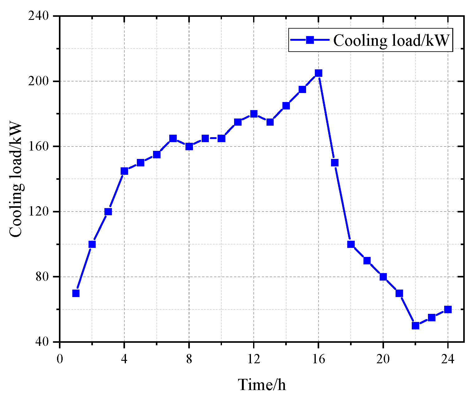
2.2.4. Cooling-Load Model

The cooling-load demand on a ship mainly originates from external infiltration heat and internal heat production. The external infiltration heat is mainly caused by the temperature difference between the external environment and the inside of the hull and is composed of two parts: high-temperature environment and solar radiation. On a clear and cloudless day, the intensity of direct solar radiation at a certain latitude perpendicular to the sun’s rays can be calculated as follows [36]:

$$i_z=I_0\frac{\sin {\alpha }_s}{\sin {\alpha }_s+\frac{1-P}{P}}$$

(56)

where $I_0$ is solar constant, ${\alpha }_s$ is solar elevation angle, and P is atmospheric transparency factor.

The direct solar intensity on the horizontal plane is:

$$i_{hor,z}=i_z\sin {\alpha }_s$$

(57)

The direct solar intensity on the vertical plane is:

$$i_{ver,z}=i_z\cos {\alpha }_s\cos \theta$$

(58)

where $\theta$ is the angle between the projection of solar radiation rays on the horizontal plane and the wall normal.

The heat transferred through the bulkhead is calculated using the reaction coefficient method [37]:

$$Q_1\left(t\right)={\displaystyle \sum }_{j=0}^{23}k\left(j\right)\Delta {\theta }_z\left(t-j\right)$$

(59)

$$\Delta {\theta }_z\left(t-j\right)={\theta }_z\left(t-j\right)-{\theta }_n$$

where ${\theta }_z\left(t-j\right)$ is the out bulkhead surface equivalent temperature at $t-j$ moment and ${\theta }_n$ is air-conditioned cabin temperature.

The heat entering the room through portholes can be calculated as follows:

$$Q_2=Q_C+Q_D+Q_f$$

(60)

where $Q_C$ is the heat transfer at any one time through the temperature difference of the porthole, $Q_D$ is the heat transfer at any one time through the convective heat transfer of the porthole, and $Q_f$ is the heat transfer at any one time through the radiant heat transfer of the porthole.

Internal heat primarily originates from artificial lighting, heat dissipation of mechanical equipment, and heat generated by the human body. The heat generated by artificial lighting is calculated as:

$$Q_3=N\phi \epsilon$$

(61)

where $N$ is the power used for lighting, $\phi$ is the usage of the lighting equipment, and $\epsilon$ is the coefficient of power consumption, which incandescent lamps are 1 and fluorescent lamps are 1.25.

The heat dissipation of mechanical equipment can be estimated as:

$$Q_4\approx 10\%Q_{total}$$

(62)

The heat generated by the human body can be estimated as:

$$Q_5\approx n_r{q}_r$$

(63)

where $n_r$ is the number of people and $q_r$ is the heat dissipation per capita.

The cooling load of the ship at any time can be calculated as:

$$Q_{total}=\sum Q_i$$

(64)

2.3. Multi-Objective Optimization

2.3.1. Methods of Optimization and Decision-Making

Figure 2 depicts the algorithm flow for loop multi-objective optimization, which involves initial parameter setting, decision variable setting, objective function setting, and the corresponding solution algorithm. Due to the complexity of the multi-objective problem, this paper adopts the Multiple Objective Particle Swarm Optimization (MOPSO) method proposed by Coello et al. [38,39,40] to find the optimal solution set of the Pareto-optimal set [41]. The main steps for searching optimal results using the MOPSO method are as follows:

Step 1: Set the initial parameters, including parameters for the cycle system and MOPSO. The circle system parameters consist of the efficiency of circulating components, ambient temperature, temperature difference at the heat exchanger grip point, and cycle calculation equation. The MOPSO parameters encompass population size, velocity upper and lower bounds, inertia factor, global learning coefficient, and individual learning coefficient, which determine the algorithm’s search performance. The iteration from the i-th particle in the t generation to the t + 1 generation is obtained as follows:

$$v_{ij}\left(t+1\right)=\omega v_{ij}\left(t\right)+c_1{v}_1\left[p_{ij}\left(t\right)-x_{ij}\left(t\right)\right]+c_2{v}_2\left[p_{gj}\left(t\right)-x_{ij}\left(t\right)\right]$$

(65)

$$x_{ij}\left(t+1\right)=x_{ij}\left(t\right)+v_{ij}\left(t\right)$$

(66)

where $\omega$ is the inertia factor, $c_1$ is the personal learning coefficient, $c_2$ is the global learning coefficient, $p_{ij}$ is the individual extreme position, $p_{gj}$ is the global optimal position, and $x_{ij}$ is the current position of the particle.

Step 2: Initialize population. Generate initial decision variables based on the input parameters from Step 1.

Step 3: Calculate the fitness of each particle in the population.

Step 4: Update the particle position. Calculate and update particle velocity and position based on their fitness.

Step 5: Calculate the fitness of the particles in the new position. If the fitness is higher, update the particle position; otherwise, it remains unchanged.

Step 6: Determine whether the termination conditions are met. Terminate the search operation if they are met; otherwise, return to Step 3.

In the context of multiple objective functions, conflicts and incomparability between objectives can lead to a situation where improving one objective function inevitably weakens at least one other objective function. To address this issue, this paper adopts the Pareto frontier solution set as the objective of the MOSPO. The primary aim is to enhance at least one objective function while ensuring that the improvement does not come at the expense of worsening other objective functions. The Pareto frontier is analyzed using the Technique for Order Preference by Similarity to an Ideal Solution (TOPSIS) method, which is a widely-used decision-making approach. The TOPSIS method, proposed by Hwang [42] et al. in 1981, ranks evaluation objects based on their proximity to an idealized target. It involves selecting a satisfactory solution that is as close as possible to the positive ideal solution while being as far away as possible from the negative ideal solution. The steps to obtain the optimal solution using the TOPSIS method are as follows:

Step 1: Standardize the evaluation objects and obtain the normalization matrix z.

$$z_{ij}=\frac{x_{ij}}{\sqrt{{{\displaystyle \sum }}_{i=1}^n{x}_{ij}^2}}\left(i=1,2,\dots ,m;j=1,2,\dots ,n\right)$$

(67)

Step 2: Identify the defined maximum and minimum values.

$$z_m^{+}=\max \left\{z_{1m},z_{2m},\dots ,z_{nm}\right\}$$

(68)

$$z_m^{-}=\min \left\{z_{1m},z_{2m},\dots ,z_{nm}\right\}$$

(69)

Step 3: Calculate the distance from the maximum and minimum values of the i-th evaluation object.

$$D_i^{+}=\sqrt{{\displaystyle \sum }_{j=1}^m{\left(z_j^{+}-z_{ij}\right)}^2}$$

(70)

$$D_i^{-}=\sqrt{{\displaystyle \sum }_{j=1}^m{\left(z_j^{-}-z_{ij}\right)}^2}$$

(71)

Step 4: Calculate the relative proximity value $R_i$ for each evaluation object. The higher the relative proximity value, the better the evaluation object.

$$R_i=\frac{D_i^{-}}{D_i^{+}+D_i^{-}}$$

(72)

2.3.2. Objective Functions and Decision Variables

In the CPDCC, once the circulating cooling capacity is determined, the analysis of this thermodynamic cycle involves three mutually constraining values: cycle comprehensive efficiency, output work, and required heat-exchanger area. The corresponding optimization goal is defined as:

$$F\left(X\right)={\left[\max \left({\eta }_{ce}\right),\max \left(W_{net}\right),\min \left(A_{total}\right)\right]}^T$$

Among them, the comprehensive efficiency is the energy-utilization rate obtained by comprehensively considering the refrigerator exergy and the heat exergy. The net output work is the external work produced by the turbine, and the heat exchanger area denotes the area required for the energy conversion process. The decision variables for the optimization include four key parameters: generation temperature, condensate temperature, mass fraction of ammonia at the generator inlet, and generator reflux. The basic parameters for multi-objective particle swarm optimization are presented in

Table 1. Initial parameters of MOPSO.

Parameters	Values
Maximum number of iterations	1000
Population size	500
Inertia factor $\omega$	0.5
Inertia factor-damping rate	0.99
Personal learning coefficient $c_1$	0.5
Global learning coefficient $c_2$	0.5

.

$$X={\left[T_h,T_c,w,R_{reflux}\right]}^T$$

The algorithm logic and flow of optimization model are illustrated in Figure 2. The green part on the left is the MOPSO process. First, the maximum number of iterations, population size, inertia factor, inertia coefficient-damping rate and learning factor need to be input. Next, the limit of the decision variable is given and the variable is initialized. Then, after obtaining the performance parameters of the thermal cycle through thermodynamic calculation, the fitness is calculated and compared. If the fitness is better, the solution set is updated. Finally, when the maximum number of iterations is reached, the Pareto front solution set is updated.

The right part is the calculation logic of the thermal cycle. Firstly, input the parameters of the fixed components in the cycle, such as isotropic efficiency, evaporation temperature, heat exchanger pinch-point temperature, and LMTD. Secondly, thermodynamic calculation is carried out by obtaining the decision variables in the MOPSO cycle. The calculation process of thermodynamics should follow the first and second laws of thermodynamics. Finally, according to the parameters of the state points, the thermodynamic performance of the cycle is calculated and input into the MOPSO cycle calculation process.

2.3.3. Model Based Assumptions

The cycle model established in this paper makes the following assumptions, based on reasonable simplification and convenience for performance analysis:

(1)

Pressure loss and energy loss in the pipes and all heat exchangers are negligible.

(2)

Chemical reactions that may occur during the cycle of working fluids are ignored.

(3)

The heat source (diesel engine exhaust), the cold source (surface seawater), and the cycle working fluid are assumed to be in a stable and uniform flow state.

(4)

The heat exchanger is assumed to have a certain heat exchange temperature difference.

(5)

The outlets of the evaporator, condenser, and absorber are all assumed to be saturated.

2.3.4. Model Validation

To verify the accuracy of the model, this paper was divided into the Kalina cycle model and the absorption refrigeration model, and the results were compared with those of other studies [43,44]. Due to different mathematical model assumptions, different heat exchanger calculation models, and different working medium physical properties database, there must be some errors for the calculation of the same cycle, and the existence of these errors is acceptable. Therefore, the error of cycle performance calculation is acceptable within 3%, and the mathematical model in this paper is reliable.

The Kalina cycle parameters and results are presented in

Table 2. Kalina cycle parameters.

Parameters	Values	Unit
Heat source temperature	28	°C
Evaporation temperature	25	°C
Cold source temperature	4	°C
Condensation temperature	8.3	°C
Pinch Point	1.5	°C
Mass fraction of ammonia	94	%
Pump isentropic efficiency	80	%
Turbine isentropic efficiency	80	%
Evaporation pressure	900	kPa

and

Table 3. Kalina cycle validation results.

Results	Units	Results in This Paper	Ref. [43]	Relative Error
Net output work	kW	9646.7	9637.12	0.10%
Thermal efficiency	%	2.09	2.05	1.95%

. The net output work and thermal efficiency of the cycle were selected as the comparison values, and the maximum relative error reached 1.95%, which is considered credible in this model.

The cycle parameters and results are presented in

Table 4. Absorption refrigeration cycle parameters.

Parameters	Values	Unit
Heat source temperature	160	°C
Cold source temperature	32	°C
Evaporator temperature	−15	°C
Mass fraction of ammonia	30.2	%
Mass flow	66.6	kg/h

and

Table 5. Absorption refrigeration cycle validation results.

Results	Units	Results in This Paper	Ref. [44]	Relative Error
Cooling capacity	kW	3.21	3.23	0.62%
COP	%	42.16	42.5	0.8%

. The cooling capacity and COP of the cycle were selected as the comparison values, and the maximum error reached 0.8%, which is considered credible in this model.

2.4. Economic Analysis of Desalination

The −18 °C cold capacity generated by the CPDCC can be utilized as a pretreatment module for RO desalination, serving in the two-stage freezing-assisted for desalination. In previous experimental studies [24,26], 35 ppt of seawater could be pre-desalinated to approximately 11 ppt through secondary freezing desalination. In this pre-desalination process, seawater is frozen in the first stage, and part of the frozen sea ice is melted in an ice melting tank, while the unfrozen seawater is passed into a mixing pipeline. Subsequently, the melted medium-concentration seawater undergoes secondary freezing. The partially frozen sea ice is then placed in another melting tank, and the resulting low-salinity seawater enters the RO desalination unit, whereas the unfrozen seawater is conveyed into the mixing pipeline. The cold in the low-temperature seawater within the mixing pipeline, the cold released during the melting process of the ice melting tank, and the low-temperature and low-concentration seawater obtained after secondary desalination can be utilized to exchange heat with the air conditioning end for cold energy recovery. The economic analysis of the seawater desalination module mainly comprises the cooling capacity consumed by frozen seawater, the cooling capacity released during the ice-melting process, electricity-consumption cost, and membrane-replacement cost.

During the first stage of the seawater-freezing process, approximately 41.8% of the seawater is frozen, and the amount of cold consumed during this process can be calculated as follows:

$$Q_{f,I}=m_{total}{c}_{seawater}\left(t_0-t_{fp1}\right)+0.418m_{total}{q}_{lat}$$

(73)

where $m_{total}$ is the total mass flow of seawater entering the desalination system, $c_{seawater}$ is the specific heat capacity of seawater, $c_{seawater}=3.89\mathrm{kJ}/\left(\mathrm{kg}·℃\right)$, $t_0$ is surface sea water temperature, $t_{fp}$ is the freezing temperature of seawater at the corresponding salinity, $q_{lat}$ is latent heat of phase change in seawater, and $q_{lat}=334 \mathrm{kJ}/\mathrm{kg}$.

After the first stage of seawater freezing, it enters the ice melting tank where it exchanges heat with the air conditioner to reach 10 °C. Subsequently, it undergoes the second stage of seawater freezing, during which approximately 24.4% of the seawater is frozen, and the amount of cold consumed during this process can be calculated as follows:

$$Q_{f,II}=0.418m_{total}{c}_{seawater}\left(t_{ac}-t_{fp2}\right)+0.244m_{total}{q}_{lat}$$

(74)

where $t_{ac}$ is the temperature of air conditioner and $t_{ac}=10 ℃$.

The total amount of cold consumption can be calculated as follows:

$$Q_f=Q_{f,I}+Q_{f,II}$$

(75)

The amount of cold recovered from the first stage of frozen-seawater-melting ice can be calculated as follows:

$$Q_{melt,I}=0.418m_{total}{q}_{lat}$$

(76)

The amount of cold recovered from the second stage of frozen-seawater-melting ice can be calculated as follows:

$$Q_{melt,II}=0.244m_{total}{q}_{lat}$$

(77)

The amount of cold recovered from low-temperature seawater recovery can be calculated as follows:

$$Q_{low}=c_{seawater}\left(m_{total}-m_{fresh}\right)\left(t_{ac}-t_{fp1}\right)$$

(78)

The total recovered cold capacity can be calculated as follows:

$$Q_{rec}=Q_{melt,I}+Q_{melt,II}+Q_{low}$$

(79)

The cost of electricity consumed by reverse osmosis devices can be calculated as follows:

$$F_E=F_1{M}_{\mathrm{p}}{M}_h$$

(80)

where $F_1$ is the cost per unit of electricity consumption, $M_{\mathrm{p}}$ is the operating power of RO equipment, and $M_h$ is the duration of RO equipment running.

Membrane-replacement costs [45] can be calculated as follows:

$$F_{RO}=0.723M_{RO}{M}_c^{-1}{M}_{ls}^{-1}$$

(81)

where $M_{RO}$ is the cost of the RO membrane, $M_C$ is the output of fresh water ($\mathrm{gal}/\mathrm{d},1 \mathrm{gal}=3.785 \mathrm{L}$), and $M_{ls}$ is the service life of the RO membrane.

The total cost of reverse osmosis desalination can be calculated as follows:

$$F_{\mathrm{T}}=F_E+F_{\mathrm{RO}}+F_{\mathrm{o}}$$

(82)

where $F_{\mathrm{o}}$ is other costs, including the cost of materials and reagents, etc., general RO takes 2 ¥/d, and pre-desalination RO takes 1 ¥/d.

3. Results and Discussions

3.1. Cycle Performance under Initial Working Conditions

For instance, considering a ship sailing near the 15° north latitude, its diesel engine power is 7500 kW, and approximately 25.7% of the energy is in the form of diesel exhaust, with the estimated total cooling capacity of the diesel engine being 600 kW [46]. Figure 3 shows the estimation of the cooling load required for a ship in a 24 h period, based on the temperature of a given day.

Figure 3 shows that the ship’s air conditioner experiences high cooling load at noon, reaching a maximum of 205 kW. At night, the cooling load decreases due to lower ambient temperature, personnel resting, and the switch-off of some lighting, resulting in reduced cooling demand for the ship. Therefore, optimizing the ship’s cycle at different times is essential. Controlling the flow of working fluid to 5 points and 11 points can be achieved through the valve after 4 points. During high cooling-load demand, the working fluid mass flow rate for air conditioning desalination is increased. Conversely, during low cooling-load demand, the working fluid mass flow rate for refrigeration desalination is increased to enhance the refrigeration coefficient and system comprehensive efficiency. Additionally, to ensure a safety margin for the ship’s cooling load, the cooling load of the ship’s air conditioner is produced using 110% of the calculated cooling-load demand.

Table 6. Initial Parameters of the CPDCC.

Parameters		Values	Unit
Generation temperature		200	°C
Seawater temperature		25	°C
Ammonia mass fraction		40	%
Reflux ratio		3.5	—
Pump isentropic efficiency		0.85	—
Turbine isentropic efficiency		0.85	—
Desalination temperature		−18	°C
Air conditioning temperature		10	°C
Temperature drops of distillation		5	°C
Pinch point	Generator	5	°C
	Absorber	5	°C
	Superheat	5	°C
	Evaporator	2	°C
	Condenser	2	°C
LMTD	Heat exchange I	5	°C
	Heat exchange II	15	°C
	Heat exchange III	15	°C

shows the initial parameters for the CPDCC.

The performance of the CPDCC at various times is depicted in Figure 4. Among them, Figure 4a presents the COP value and comprehensive efficiency of the CPDCC within 24 h. It is evident that as the ship’s cooling load demand increases, i.e., with an increase in the mass flow of working fluid entering the air conditioning cycle, COP decreases, leading to a decline in the system’s comprehensive efficiency. Conversely, a higher mass flow rate of the working fluid entering seawater-freezing desalination results in an increased circulating COP value and comprehensive efficiency of the system. Figure 4b illustrates the air conditioning cooling capacity and the cooling capacity used for desalination in CPDCC. At 4 p.m., the cooling-load demand for the ship is at its maximum, resulting in the highest air conditioning cooling capacity of 225.5 kW. As the demand for the cooling load of the ship’s air conditioning rises, the total cooling capacity of the ship decreases, peaking at 613.53 kW at 22 o’clock.

Table 7. Calculation results of the CPDCC under the initial working conditions.

State Points	Temperature	Pressure	Specific Enthalpy	Specific Entropy	Mass Flow	Mass Fraction
	°C	MPa	kJ/kg	kJ/(kg·K)	kg/s	%
1	190	3.28	2007.68	6.28	0.5199	100
2	195	3.28	2021.33	6.31	0.5199	100
3	105.91	1.07	1839.14	6.40	0.5199	100
4	27	1.07	470.43	1.91	0.5199	100
5	27	1.07	470.43	1.91	0.1954	100
6	24.69	1.07	459.34	1.88	0.1954	100
7	8	0.57	459.34	1.89	0.1954	100
8	8	0.57	1613.43	5.99	0.1954	100
9	12	0.57	1624.52	6.03	0.1954	100
10	−0.30	0.22	1624.52	6.47	0.1954	100
11	27	1.07	470.43	1.91	0.3245	100
12	11.31	1.07	396.11	1.66	0.3245	100
13	−20	0.19	396.11	1.70	0.3245	100
14	−20	0.19	1580.83	6.38	0.3245	100
15	12	0.19	1655.15	6.65	0.3245	100
16	21.75	0.22	1675.11	6.65	0.3245	100
17	195	3.28	803.52	2.57	1.2997	16
18	35.38	3.28	77.29	0.69	1.2997	16
19	36.00	0.22	77.29	0.70	1.2997	16
20	30	0.22	28.11	0.839	1.8196	40
21	30.38	3.28	32.32	0.841	1.8196	40
22	138.21	3.28	551.05	2.30	1.8196	40

and

Table 8. Cycle performance under the initial working conditions.

Components	Values	Unit	Components	Values	Unit
$Q_{gen}$	1085.42	kW	$W_{com,II}$	6.48	kW
$Q_{re}$	7.10	kW	$W_{tur}$	94.72	kW
$Q_{con}$	711.57	kW	$W_{net}$	80.58	kW
$Q_{eva,I}$	225.50	kW	COP	55.83	%
$Q_{eva,II}$	383.79	kW	${\eta }_{power}$	7.38	%
$Q_{abs}$	903.30	kW	${\eta }_{ce,power}$	19.94	%
$W_{pump}$	7.66	kW	${\eta }_{ce,ref}$	17.54	%
$W_{com,I}$	—	—	${\eta }_{ce}$	37.48	%

present the cycle state point parameters and various performance parameters of the CPDCC when the vessel’s cooling load reaches its maximum, respectively. Under this working condition, the net output work is 80.58 kW, with a thermal efficiency of 7.38%, a COP of 55.83%, and a comprehensive efficiency of 37.48%.

The parameter diagram of each point of the CPDCC when the cooling load of the ship reaches its maximum is shown in Figure 5. In the diagram, 22-1-2 represents the heating section, where the working fluid is absorbed by the generator and reheater. The turbine in the 2–4 section experiences the external output work, and then the working fluid is condensed to the saturated liquid state through the condenser. Subsequently, two sub-loops, 5–10 and 11–16, are entered. The 5–10 sub-cycle is responsible for air conditioning refrigeration, while the 11–16 sub-cycle focuses on desalination. Finally, the working fluid is mixed with concentrated ammonia–water in the absorber to obtain saturated dilute ammonia.

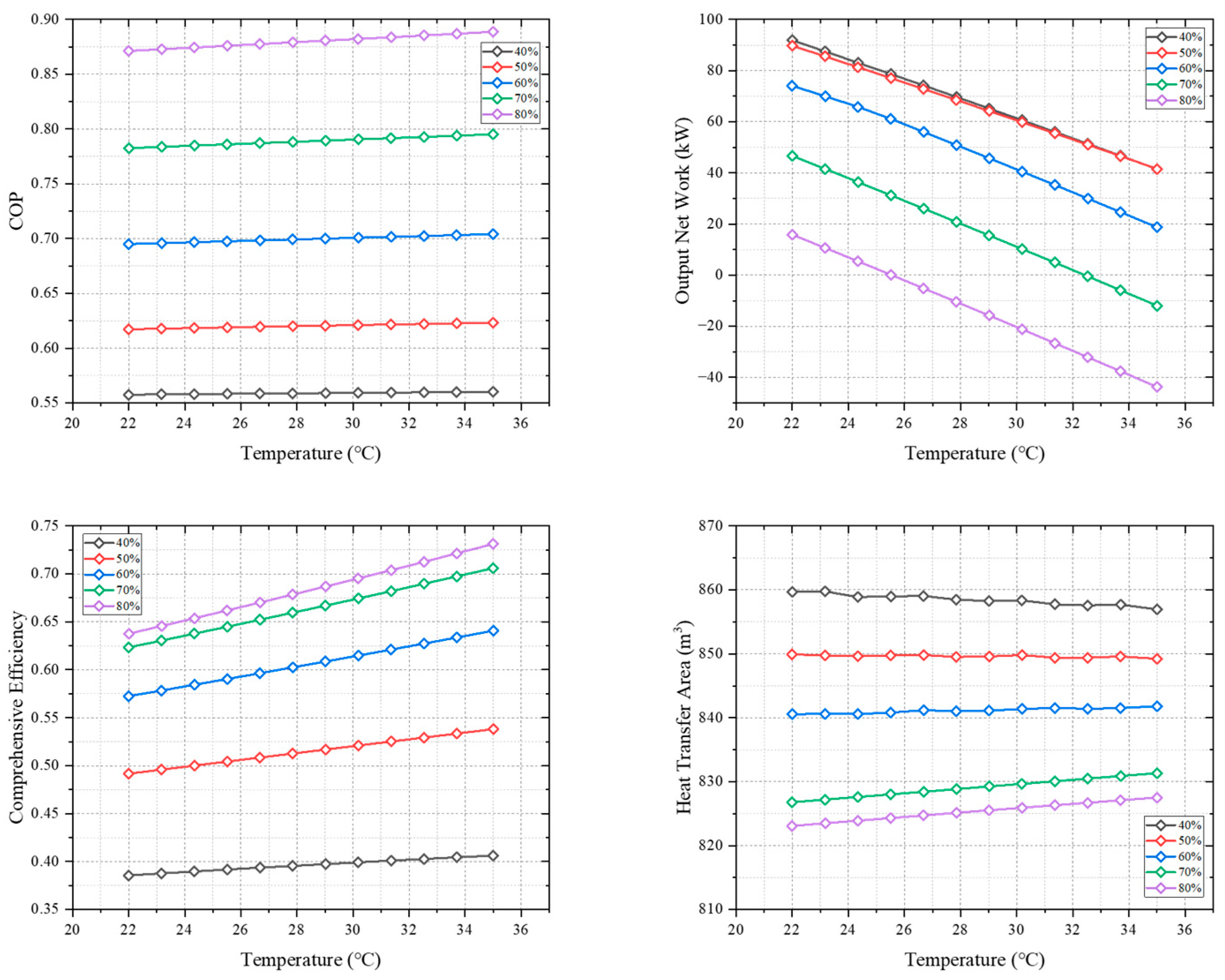
3.2. Cycle Performance under Variable Working Conditions

During the ship’s voyage, the temperature of the ship’s diesel exhaust gas fluctuates, and the temperature of different sea areas changes over time. The system’s performance is significantly affected by the mass concentration of ammonia and the reflux ratio of the generator [18].

The temperature of marine diesel exhaust generally stays below 550 °C. It usually undergoes a thermal cycle for heat recovery, where the temperature typically ranges between 150~250 °C. The variation in generation temperature significantly impacts the cycle’s performance [47]. Due to the varying mass fractions of ammonia and their different performances at different temperatures during the CPDCC, Figure 6 illustrates the cycle’s performance under different generation temperatures. It is evident that with an increase in generation temperature, the output work increases, while the COP value decreases, leading to a larger heat exchanger area. Changes in the mass fraction of ammonia in the working fluid also influence the working performance of the CPDCC. Increasing the mass fraction of ammonia leads to a rise in absorption pressure and compressor power consumption. However, when the heat source temperature is below 200 °C, the functional power of 80% concentration of ammonia–water cannot meet the system’s power consumption requirements. Usually, the larger the mass fraction of ammonia, the better the system’s performance parameters. However, as the generation temperature increases, high concentrations of ammonia are no longer suitable as a cycling working medium, leading to reduced working performance. Specifically, the performance of the working fluid with an 80% mass fraction of ammonia is significantly diminished. When the generation temperature reaches 230 °C, the COP value of the cycle significantly drops, resulting in a net output work lower than that of the low concentration of ammonia–water solution. Additionally, a larger heat exchanger area is required.

In different sea areas and at different times, the temperature of the seawater surface varies significantly. For example, in the sea near the equator in Southeast Asia, the sea temperature can reach approximately 30 °C. Figure 7 presents data from the National Oceanic and Atmospheric Administration (NOAA) and the Climate Change Institute at the University of Maine, released on 1 July 2023 and 10 December 2023 [48]. During the summer and winter seasons, the sea water temperature near the equator in Southeast Asia remains at approximately 30 °C, while the surface sea water temperature along the southeast coast of China is above 25 °C in the summer and above 22 °C in the winter. Figure 8 illustrates the performance parameters of the CPDCC when different mass fractions of ammonia are used as working fluids, with a cold source temperature range of 22~35 °C. As the seawater temperature and ammonia mass fraction increase, the COP value and comprehensive efficiency of the CPDCC improve, leading to a reduction in the required heat exchanger area. However, the net output work decreases due to the decreased temperature difference between the heat source and the reduced Carnot efficiency as the seawater temperature rises. Increasing the mass concentration of ammonia can alleviate this issue. However, when the mass concentration of ammonia reaches 80%, the net output work of the system decreases as the seawater temperature rises. At a seawater temperature of 26 °C, the output work of the system cannot meet the self-sufficiency demand.

The reflux ratio represents the ratio between the mass flow rate of the working fluid entering the generator and the mass flow rate of pure distilled ammonia in the distillation column:

$$R_{reflux}=\frac{m_{22}}{m_1}$$

(83)

The magnitude of the reflux ratio significantly influences the mass fraction of dilute ammonia and the mass flow rate of the distillate product in the distillation column. A variable working condition analysis is conducted for reflux ratio values ranging from 2.5 to 4. As the reflux ratio increases, the mass flow rate of pure distilled ammonia in the distillation column increases, leading to a decrease in the concentration of distilled dilute ammonia. Consequently, the system’s net output work increases, and the required heat exchanger area also increases. Figure 9 shows the performance parameters of ammonia with various mass fractions at different reflux ratios. It is evident that as the reflux ratio increases, the net output work of the low-concentration ammonia–water system increases, whereas the net output work of the high-concentration ammonia–water system decreases. The 60% concentration of ammonia–water remains almost unaffected, and its influence on the system’s overall efficiency gradually approaches an intermediate value. With a given reflux ratio, increasing the mass fraction of ammonia to 60–80% results in improved COP, comprehensive efficiency, and reduced heat exchanger-area requirements for the system. The variation in reflux ratio has minimal impact on the COP value of the CPDCC; instead, it primarily influences the cycle’s thermodynamic performance and heat transfer area.

The variation in reflux ratio has minimal impact on the COP value of the CPDCC; instead, it primarily influences the cycle’s thermodynamic performance and heat transfer area. However, as the absorption pressure varies with different concentrations of ammonia–water, when the absorption pressure exceeds the evaporation pressure, a gas compressor is necessary to raise the vapor pressure to the absorption pressure level. Thus, the net output work of the system must be taken into account. While high-concentration ammonia exhibits good energy-conversion efficiency, the high absorption pressure results in high power consumption for the compressor, which often fails to meet the power consumption requirements of the system itself. The cooling capacity generated by the cycle is nearly constant. Therefore, an increase in the temperature difference between the generation temperature and the cold source temperature leads to a rise in the total heat absorption of the system and a decrease in the COP value of the system. Cooling and output work represent two distinct energy grades; hence, the cycle’s performance should be analyzed from the exergy analysis perspective, considering the system’s comprehensive efficiency. Additionally, employing ammonia with a higher mass fraction as the working fluid can substantially enhance the cycle’s performance while reducing the required heat exchanger area. However, caution should be exercised not to use an excessively high mass fraction of ammonia, as it would result in a decrease in the system’s output functional force. Appropriate concentrations of ammonia should be selected based on different temperatures.

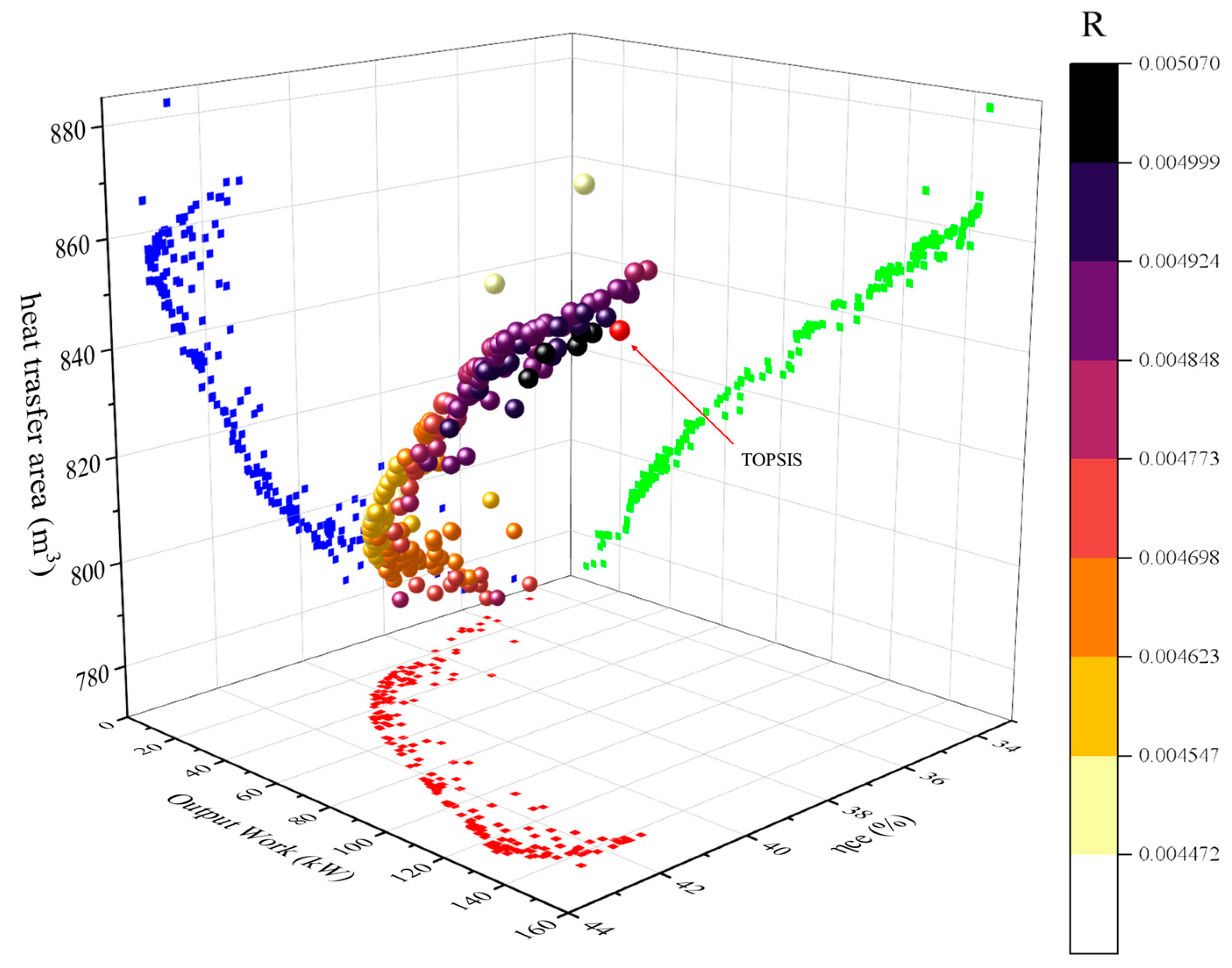
3.3. Multi-Objective Optimization Results and Analysis

The previous part of the study indicated that various performance parameters of the cycle are affected differently by generation temperature, cold source temperature, mass fraction of ammonia, and reflux ratio, and this effect is complex. Therefore, the MOPSO algorithm is selected to optimize and analyze these four independent decision variables. The optimization objectives are to select the net output work, the comprehensive efficiency of cycle, and the total heat exchanger area. The higher the net output work, the stronger the cycle’s work capacity. The higher the comprehensive efficiency of the cycle, the better the cycle’s exergy-utilization rate. The lower the total heat exchanger area, the better the cycle’s economy, and the lower the investment cost. Among them, in the case of higher generation temperature, the working boundary of part of the ammonia working fluid is exceeded, so the generation temperature range is selected from 150 °C to 250 °C. In non-extreme weather, the sea-surface temperature near Southeast Asia generally does not exceed 30 °C. Therefore, the cold source temperature range is set from 22 °C to 30 °C. Since the mass fraction of ammonia–water has a significant influence at different temperatures, 30–80% ammonia concentration is selected for multi-objective analysis. The range of values of independent decision variables is shown in

Table 9. The value range of the decision variable.

Parameter	Values	Unit
Generation temperature	150~250	°C
Seawater temperature	22~30	°C
Ammonia mass fraction	0.3~0.8	-
Reflux ratio	2.5~4	-

. As shown in Figure 10, the MOPSO algorithm yields a large number of non-dominated solutions, forming a Pareto frontier solution set. To further search for the Pareto optimal solution, we introduced the Technique for Order Preference by Similarity to an Ideal Solution (TOPSIS) method to rank the advantages and disadvantages of the solutions. The output at the maximum or minimum value of the optimization target is shown in

Table 10. The optimization results of MOPSO.

Optimal Values		Design Variables				Optimize Goals
		Th/°C	Tc/°C	w	Rreflux	Wnet/kW	ηce/%	Atotal/m3
Wnet	max	249.46	22.27	0.407	3.60	144.70	42.67	882.54
	min	156.29	23.35	0.794	3.12	6.46	34.58	773.23
ηce	max	248.54	22.01	0.498	3.42	125.96	43.25	865.77
	min	156.29	23.35	0.794	3.12	6.46	34.58	773.23
Atotal	min	156.29	23.35	0.794	3.12	6.46	34.58	773.23
	max	249.46	22.27	0.407	3.60	144.70	42.67	882.54
TOPSIS results		249.95	22.29	0.420	3.24	142.08	42.34	863.32

. The visual output of the Pareto frontier is shown in Figure 10, where the color from light to dark indicates the inferior to the best of the set of understandings, and the optimal value is represented by a red ball. When the temperature reaches 249.95 °C, the cold source temperature reaches 22.29 °C, the mass fraction of ammonia reaches 42.0%, the reflux ratio is 3.24, the comprehensive performance of the system is better, the net output work reaches 142.08 kW, the comprehensive efficiency reaches 42.34%, and the area demand of the heat exchanger is low, which is 862.32 m³.

3.4. Exergy Analysis

The exergy flow diagram of the system is shown in Figure 11. The exergy loss of each component of the system is provided, including both the utilized exergy and the irreversible exergy loss. Under the highest cooling-load operation of the system, the comprehensive efficiency reached 42.34%, with 13.50% attributed to cooling exergy and 28.84% to power exergy. The system experienced an irreversible loss of 57.66%, primarily concentrated in components such as evaporators and generators that underwent endothermic phase transitions. In the evaporator, the output process of cold energy is primarily associated with an increase in entropy, resulting in a total exergy loss of 14.15% for the two evaporators. Before entering the generator, the ammonia–water is heated to a certain extent, which alleviates the irreversible loss in the generator, reaching 24.01%. Typically, irreversible losses in the generator are caused by the phase transition of the fluid inside the generator. The working fluid at the generator inlet has a temperature of approximately 140 °C, which creates a significant temperature difference with the external heat source and results in a significant irreversible loss. The heat exchange between the ammonia–water before entering the generator and the high-temperature dilute ammonia–water distilled by the generator results in an irreversible loss of 5.99%. Additionally, in the absorber, the absorption process of ammonia releases a significant amount of heat. To ensure the absorption capacity of ammonia–water, the absorber is cooled by cooling water, which results in a significant irreversible loss of 7.11%. The turbine, pump, condenser, compressors, and reheater exhibit irreversible losses of 0.35%, 0.92%, 1.36%, 3.46%, and 0.17%, respectively.

3.5. Performance Comparison between the CPDCC and other Cycles

Table 11. Comparison between CPDCC and other cycles.

Years	Fluids	Thot	Tcold	Teva	ηpower	COP	ηce	Ref.
		°C	°C	°C	%	%	%
2008	NH3-H2O	300	20	−5	14.96	5.49	36.60	[49]
2013	NH3-H2O	28	4		2.94		36.89	[50]
2015	NH3-H2O	75	4	−18	2.27	18.00	22.29	[51]
2019	NH3-H2O (Power) R600a (Refrigeration)	122	4.85	8	8.00	24.00	50.34	[52]
2021	Cyclopentane–Toluene	200	5		23.00		49.21	[53]
2023	NH3-H2O	30	5	−18	0.85	29	66.14	[28]
2023	NH3-H2O	249.95	22.29	10, −18	12.55	54.36	42.34	CPDCC

presents the performance comparison between the proposed CPDCC and other types of waste heat utilization cycles. Compared to the traditional organic Rankine cycle, the CPDCC exhibits a lower thermal efficiency of 12.55%. This is attributed to the use of a slightly higher mass fraction of ammonia as the working fluid and the utilization of part of the output work in the air compressor to increase the vapor pressure after the evaporator. Simultaneously, although employing a high mass fraction of ammonia results in an increase in absorption pressure, it significantly enhances the cycle’s COP value. The CPDCC is capable of achieving two different cooling temperatures of 10 °C and −18 °C simultaneously, serving for air conditioning and desalination purposes, respectively. The CPDCC exhibits a comprehensive efficiency of 42.34%, primarily due to the significant irreversible loss generated by the entropy production unit (evaporator), and the insufficient heating of ammonia entering the generator leads to a high irreversible loss in the generator.

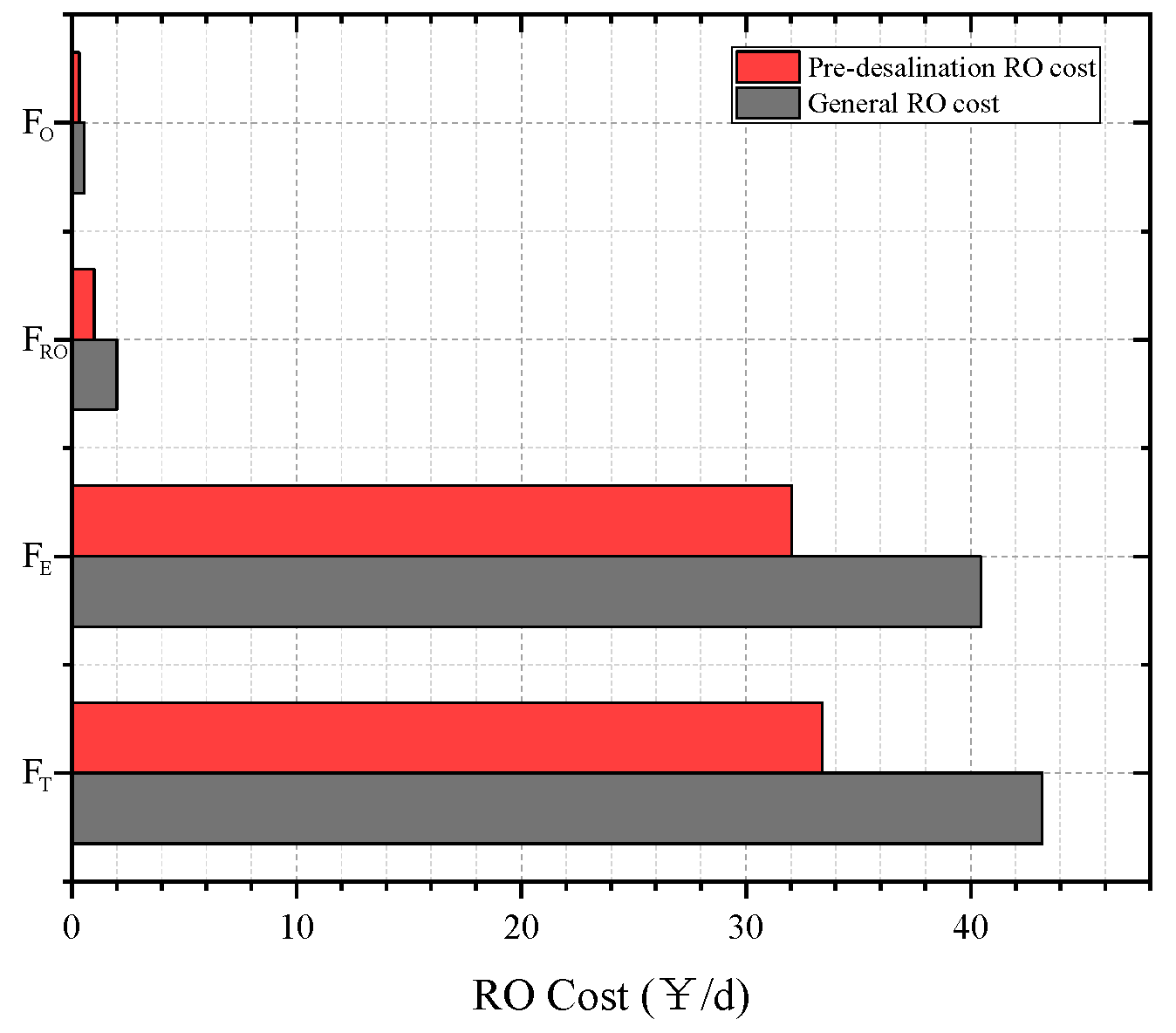
3.6. Economic Analysis of Desalination

According to Formulas (73)–(79), the seawater flow treated by the seawater pre-desalination system and the cold amount recovered in a single day can be calculated. It is estimated that approximately 70% of the cold capacity can be effectively utilized in the seawater-freezing press. Figure 12 shows the expected production of low-salinity seawater and the recovery of cold water in one day. It is expected that the desalination system will produce 7089 L of fresh water per day, with a cold recovery rate of 55.39%, and that the recovered cold energy can be used for air conditioning cooling or storage.

Previous experimental studies have shown that reducing the salinity of seawater at the desalination equipment inlet results in lower operating power for the RO equipment [26]. The RO system operating with ordinary seawater of 35 ppt salinity reaches 94.74% of the rated power, while the RO system with 11 ppt salinity operates at 74.74% of the rated power. The YB-SWRO-100TPD desalination equipment is rated at 33 kW, and with 35 ppt and 11 ppt brine, its operating power is 31.26 kW and 24.66 kW, respectively. The unit electricity consumption cost is 1.3 ¥/kWh due to the high cost of diesel engine power generation. The electricity consumption cost for ordinary RO and pre-desalination RO is calculated to be 40.64 ¥/d and 32.06 ¥/d, respectively. Additionally, the RO equipment can supply the power required for its operation through the CPDCC without the need for additional circuitry. According to study [45], under high-concentration and high-pressure working conditions, the service life of a general RO membrane is 3 years. However, after pre-desalination treatment, the service life of the RO membrane can be extended to 5 years under low-salinity and low-pressure working conditions. The YB-SWRO-100TPD desalination equipment has a cost of 603 $/unit for the RO membrane, a recovery rate of 35% for the RO equipment, and an expected freshwater output of 7089 L/d (1872.7 gal/d). The replacement costs of general RO and pre-desalination RO membranes are 0.55 ¥/d and 0.33 ¥/d, respectively. Figure 13 shows the different costs between pre-desalination RO and general RO. According to Equations (81)–(83), when using YB-SWRO-100TPD desalination equipment, the total cost of general RO is 43.19 ¥/d, and the total cost of pre-desalination RO is 33.39 ¥/d, which can save about 22.69%.

4. Conclusions

This paper proposes a novel cooling-power-desalination combined cycle (CPDCC) for recovering shipboard diesel exhaust heat, integrating a freezing desalination sub-cycle to regulate the ship’s cooling-load fluctuations. Moreover, the refrigeration produced by this cycle is ingeniously utilized for the pretreatment of RO desalination. To assess the cycle’s performance under variable working conditions, we established a comprehensive mathematical model and conducted both energy and exergy analyses. Subsequently, we performed multi-objective optimization using the MOPSO technique and compared the results with those of other cycles. Furthermore, an economic analysis was carried out to evaluate the cycle’s economic viability. The main conclusions can be summarized as follows:

(1)

The performance of CPDCC is significantly influenced by the mass fractions of ammonia–water solution. Opting for a higher concentration ammonia–water solution enhances the heat conversion performance and efficiency of the cycle. However, it also leads to an increase in the cycle absorption pressure, which necessitates the use of an additional air compressor to raise the vapor pressure, resulting in a reduction in the cycle’s net output work.

(2)

After conducting MOPSO multi-objective optimization, considerable improvement is achieved in CPDCC performance, with a thermal efficiency of 12.55%, a COP of 54.36%, and a comprehensive efficiency of 42.34%. Notably, there is still potential for further enhancing the output work by considering the heat exchanger area.

(3)

The main exergy losses in the CPDCC occur in the evaporators, generator, and absorber, accounting for 78.51% of the total exergy losses in the system.

(4)

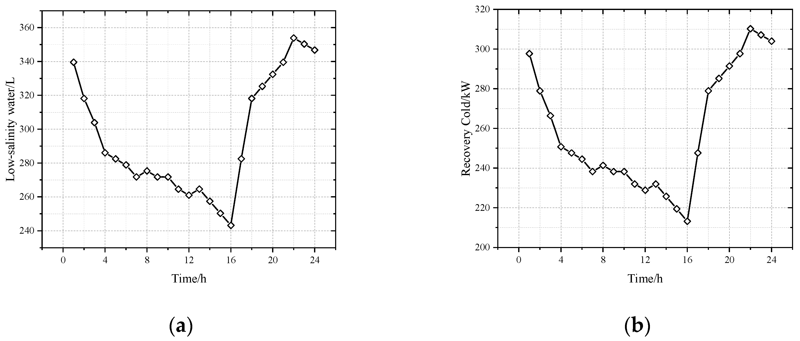
After multi-objective optimization, the net output power of the CPDCC is 142.08 kW, the total heat exchange area of each heat exchange component is 863.32 m2, and it is expected that the maximum output of fresh water is about 7000 per day. The implementation of freezing desalination significantly reduces the cost of RO desalination by 22.69%, the cold recovery rate reaches 55.39%, and the power generated by CPDCC can meet the needs of RO desalination equipment.

References

1. Mondejar, M.E.; Andreasen, J.G.; Pierobon, L.; Larsen, U.; Thern, M.; Haglind, F. A review of the use of organic Rankine cycle power systems for maritime applications. Renew. Sustain. Energy Rev. 2018, 91, 126–151. [Google Scholar] [CrossRef]
2. MARPOL: Annex VI and NTC 2008 with Guidelines for Implementation; IMO: London, UK, 2013; Volume 258.
3. International Convention for the Prevention of Pollution from Ships (MARPOL). 2005. Available online: https://www.imo.org/en/about/Conventions/Pages/International-Convention-for-the-Prevention-of-Pollution-from-Ships-(MARPOL).aspx (accessed on 30 October 2023).
4. Song, J.; Song, Y.; Gu, C.-w. Thermodynamic analysis and performance optimization of an Organic Rankine Cycle (ORC) waste heat recovery system for marine diesel engines. Energy 2015, 82, 976–985. [Google Scholar] [CrossRef]
5. Yang, M.-H.; Yeh, R.-H. Thermodynamic and economic performances optimization of an organic Rankine cycle system utilizing exhaust gas of a large marine diesel engine. Appl. Energy 2015, 149, 1–12. [Google Scholar] [CrossRef]
6. Yang, M.-H. Thermal and economic analyses of a compact waste heat recovering system for the marine diesel engine using transcritical Rankine cycle. Energy Convers. Manag. 2015, 106, 1082–1096. [Google Scholar] [CrossRef]
7. Yang, M.-H. Optimizations of the waste heat recovery system for a large marine diesel engine based on transcritical Rankine cycle. Energy 2016, 113, 1109–1124. [Google Scholar] [CrossRef]
8. Mat Nawi, Z.; Kamarudin, S.K.; Sheikh Abdullah, S.R.; Lam, S.S. The potential of exhaust waste heat recovery (WHR) from marine diesel engines via organic rankine cycle. Energy 2019, 166, 17–31. [Google Scholar] [CrossRef]
9. Feng, Y.; Du, Z.; Shreka, M.; Zhu, Y.; Zhou, S.; Zhang, W. Thermodynamic analysis and performance optimization of the supercritical carbon dioxide Brayton cycle combined with the Kalina cycle for waste heat recovery from a marine low-speed diesel engine. Energy Convers. Manag. 2020, 206, 112483. [Google Scholar] [CrossRef]
10. Sakalis, G. Investigation of supercritical CO2 cycles potential for marine Diesel engine waste heat recovery applications. Appl. Therm. Eng. 2021, 195, 117201. [Google Scholar] [CrossRef]
11. Gürgen, S.; Altın, İ. Novel decision-making strategy for working fluid selection in Organic Rankine Cycle: A case study for waste heat recovery of a marine diesel engine. Energy 2022, 252, 124023. [Google Scholar] [CrossRef]
12. Ouadha, A.; El-Gotni, Y. Integration of an Ammonia-water Absorption Refrigeration System with a Marine Diesel Engine: A Thermodynamic Study. Procedia Comput. Sci. 2013, 19, 754–761. [Google Scholar] [CrossRef]
13. Alklaibi, A.M.; Lior, N. Waste heat utilization from internal combustion engines for power augmentation and refrigeration. Renew. Sustain. Energy Rev. 2021, 152, 111629. [Google Scholar] [CrossRef]
14. Demir, M.E.; Çıtakoğlu, F. Design and modeling of a multigeneration system driven by waste heat of a marine diesel engine. Int. J. Hydrogen Energy 2022, 47, 40513–40530. [Google Scholar] [CrossRef]
15. Shafieian, A.; Khiadani, M. A multipurpose desalination, cooling, and air-conditioning system powered by waste heat recovery from diesel exhaust fumes and cooling water. Case Stud. Therm. Eng. 2020, 21, 100702. [Google Scholar] [CrossRef]
16. Cao, Y.; Mihardjo, L.W.W.; Dahari, M.; Mustafa Mohamed, A.; Ghaebi, H.; Parikhani, T. Assessment of a novel system utilizing gases exhausted from a ship’s engine for power, cooling, and desalinated water generation. Appl. Therm. Eng. 2021, 184, 116177. [Google Scholar] [CrossRef]
17. Tang, J.; Ni, H.; Peng, R.-L.; Wang, N.; Zuo, L. A review on energy conversion using hybrid photovoltaic and thermoelectric systems. J. Power Sources 2023, 562, 232785. [Google Scholar] [CrossRef]
18. Li, X.; Xu, B.; Tian, H.; Shu, G. Towards a novel holistic design of organic Rankine cycle (ORC) systems operating under heat source fluctuations and intermittency. Renew. Sustain. Energy Rev. 2021, 147, 111207. [Google Scholar] [CrossRef]
19. Wang, M.; Zhang, Y.; Xie, J. Simulation analysis of dynamic cooling loads of ship air conditioning in summer. Chin. J. Ship Res. 2018, 13, 8. [Google Scholar]
20. Roemmich, D.; Gilson, J. The 2004–2008 mean and annual cycle of temperature, salinity, and steric height in the global ocean from the Argo Program. Prog. Oceanogr. 2009, 82, 81–100. [Google Scholar] [CrossRef]
21. Salajeghe, M.; Ameri, M. Thermodynamic analysis of single and multi-effect freeze desalination. Appl. Therm. Eng. 2023, 225, 120148. [Google Scholar] [CrossRef]
22. Janajreh, I.; Zhang, H.; El Kadi, K.; Ghaffour, N. Freeze desalination: Current research development and future prospects. Water Res. 2023, 229, 119389. [Google Scholar] [CrossRef]
23. Ali, U.; Zhang, H.; Abedrabbo, S.; Janajreh, I. Freeze desalination via thermoacoustic cooling: System analysis and cost overview. Energy Nexus 2023, 10, 100195. [Google Scholar] [CrossRef]
24. Yuan, H.; Sun, P.; Zhang, J.; Sun, K.; Mei, N.; Zhou, P. Theoretical and experimental investigation of an absorption refrigeration and pre-desalination system for marine engine exhaust gas heat recovery. Appl. Therm. Eng. 2019, 150, 224–236. [Google Scholar] [CrossRef]
25. Ni, N.; Yuan, H.; Zhang, Z.; Bai, Y.; Zhu, M. Theoretical research on ship desulfurization wastewater freezing desalination system driven by waste heat. Desalination 2023, 549, 116363. [Google Scholar] [CrossRef]
26. Sun, P.; Yuan, H.; Zhang, J.; Sun, K.; Pang, H. Experimental investigation of a seawater freezing pre-desalination system. Period. Ocean Univ. China 2021, 51, 8. [Google Scholar]
27. Song, R.; Wang, K.; Gong, M.; Yuan, H. Multi-physical field simulations of directional seawater freeze-crystallisation under a magnetic field. Desalination 2023, 560, 116687. [Google Scholar] [CrossRef]
28. Zhang, Z.X.; Yuan, H.; Mei, N. Theoretical analysis on extraction-ejection combined power and refrigeration cycle for ocean thermal energy conversion. Energy 2023, 273, 127216. [Google Scholar] [CrossRef]
29. Qian, S. Heat Exchanger Design Handbook; Chemical Industry Press: Beijing, China, 2002. [Google Scholar]
30. Shah, M.M. A general correlation for heat transfer during film condensation inside pipes. Int. J. Heat Mass Transf. 1979, 22, 547–556. [Google Scholar] [CrossRef]
31. Bivens, D.B.; Yokozeki, A. Heat Transfer Coefficients and Transport Properties for Alternative Refrigerants. In Proceedings of the International Refrigeration and Air Conditioning Conference, Hannover, Germany, 10–13 May 1994. [Google Scholar]
32. Churchill, S.W.; Bernstein, M. A Correlating Equation for Forced Convection From Gases and Liquids to a Circular Cylinder in Crossflow. J. Heat Transf. 1977, 99, 300–306. [Google Scholar] [CrossRef]
33. Du, S.; Li, Q.Y.; Cao, X.; Song, Q.L.; Wang, D.C.; Li, Y.H.; Li, L.S.; Liu, J. Investigation on heat transfer and pressure drop correlations of R600a air-cooled finned tube evaporator for fridge. Int. J. Refrig. 2022, 144, 118–127. [Google Scholar] [CrossRef]
34. Gnielinski, V. New Equations for Heat and Mass Transfer in Turbulent Pipe and Channel Flows. Int. Chem. Eng. 1976, 16, 359–367. [Google Scholar]
35. E, W. Study on Calculation Method of Ammonia-Water Absorber Area with Heat and Mass Transfer Process. Master’s Thesis, Southeast University, Nanjing, China, 2015. [Google Scholar]
36. Yang, L. Research on Frequency Conversion Energy-Saving Technology of Ship Refrigerator. Master’s Thesis, Shanghai Maritime University, Shanghai, China, 2000. (In Chinese). [Google Scholar]
37. Gao, S. Dynamic Cooling Loads of Ship Air-Condition. Master’s Thesis, Dalian University of Technology, Dalian, China, 2006. [Google Scholar]
38. Coello, C.A.C.; Lechuga, M.S. MOPSO: A proposal for multiple objective particle swarm optimization. In Proceedings of the WCCI 2002, Honolulu, HI, USA, 12–17 May 2002. [Google Scholar]
39. Eberhart, R.; Kennedy, J. A new optimizer using particle swarm theory. In Proceedings of the Mhs95 Sixth International Symposium on Micro Machine & Human Science, Nagoya, Japan, 4–6 October 2002. [Google Scholar]
40. Kennedy, J.; Eberhart, R. Particle Swarm Optimization. In Proceedings of the ICNN95—International Conference on Neural Networks, Perth, Australia, 27 November–1 December 1995. [Google Scholar]
41. Banzhaf, W.; Daida, J.; Eiben, A.E.; Garzon, M.H.; Honavar, V.; Jakiela, M.; E, R. A Comprehensive Survey of Evolutionary Based Multiobjective Optimization Techniques. Knowl. Inf. Syst. 1999, 1, 269–308. [Google Scholar]
42. Hwang, C.L.; Yoon, K. Multiple attribute decision making. Methods and applications. A state-of-the-art survey. In Lecture Notes in Economics and Mathematical Systems; Springer: Berlin, Germany, 1981; Volume 186. [Google Scholar]
43. Xue, B. Performance Analysis of Ocean Thermal Energy Convention System Using Kalina Cycle an Uehara Cycle. Master’s Thesis, China University of Petroleum, Beijing, China, 2020. [Google Scholar]
44. Zhang, X. Experimental and Simulation Study on Ammonia-Water Absorption Refrigeration. Master’s Thesis, Qingdao University of Science & Technology, Qingdao, China, 2020. [Google Scholar]
45. Gao, C.; Ruan, G. Chapter 4—Reverse osmosis and nanofiltration seawater desalination. In Seawater Desalination Technology and Engineering; American Water Works Association: Washington, DC, USA, 2016; pp. 294–301. [Google Scholar]
46. Shen, B.; Pan, X.; Wang, W. Feasibility of absorption refrigeration air conditioner powered by west heat. Navig. China 2012, 35, 33–36. [Google Scholar]
47. Luo, L.; Fan, Y.; Zhou, D.; Wang, L.; Chen, X.; Xi, G. Experimental study of waste heat recovery of diesel exhaust gas fromn small and medium-sized ships. Ship Eng. 2021, 12, 043. [Google Scholar]
48. Climate Reanalyzer. Daily Sea Surface Temperature. Climate Change Institute, University of Maine. n.d. Available online: https://climatereanalyzer.org/ (accessed on 12 December 2023).
49. Wang, J.; Dai, Y.; Gao, L. Parametric analysis and optimization for a combined power and refrigeration cycle. Appl. Energy 2008, 85, 1071–1085. [Google Scholar] [CrossRef]
50. Yuan, H.; Mei, N.; Li, Y.; Yang, S.; Hu, S.Y.; Han, Y.F. Theoretical and experimental investigation on a liquid-gas ejector power cycle using ammonia-water. Sci. China Technol. Sci. 2013, 56, 2289–2298. [Google Scholar] [CrossRef]
51. Yuan, H.; Zhou, P.; Mei, N. Performance analysis of a solar-assisted OTEC cycle for power generation and fishery cold storage refrigeration. Appl. Therm. Eng. 2015, 90, 809–819. [Google Scholar] [CrossRef]
52. Bian, Y.; Pan, J.; Liu, Y.; Zhang, F.; Yang, Y.; Arima, H. Performance analysis of a combined power and refrigeration cycle. Energy Convers. Manag. 2019, 185, 259–270. [Google Scholar] [CrossRef]
53. Gao, Q.; Yuan, H. Performance Analysis of Zeotropic Organic Rankine Cycle for Marine Diesel Exhaust Heat Recovery. In Proceedings of the ASME 2021 International Mechanical Engineering Congress and Exposition, IMECE 2021, Virtual, GA, USA, 1–5 November 2021; American Society of Mechanical Engineers (ASME): New York, NY, USA, 2021. [Google Scholar]
Figure 1. Schematic of the cooling-power-desalination combined cycle (CPDCC).
Sustainability 15 16942 g001
Figure 2. Multi-objective optimization flowchart.
Sustainability 15 16942 g002
Figure 3. Cooling load for one day.
Sustainability 15 16942 g003
Figure 4. Performance parameters of the system for one day. (a) COP and comprehensive efficiency of system. (b) The cooling capacity of the system.
Sustainability 15 16942 g004
Figure 5. CPDCC state parameter diagram. (a) T—s diagram; (b) P—T diagram; (c) P—V diagram; (d) P—h diagram.
Sustainability 15 16942 g005
Figure 6. Cycle performance parameters with different generation temperatures.
Sustainability 15 16942 g006
Figure 7. Sea-surface temperature of different sea areas. (a) Summer sea-surface temperature. (b) Winter sea-surface temperature [48]. Reprinted from Climate Reanalyzer.
Sustainability 15 16942 g007
Figure 8. Cycle performance parameters with different sea-surface water temperatures.
Sustainability 15 16942 g008
Figure 9. Cycle performance parameters with different reflux ratios.
Sustainability 15 16942 g009
Figure 10. Pareto Frontier for MOPSO solutions.
Sustainability 15 16942 g010
Figure 11. Exergy flow chart of the CPDCC.
Sustainability 15 16942 g011
Figure 12. (a) Low-salinity water produced in a single day. (b) Recovery of cold energy in a single day.
Sustainability 15 16942 g012
Figure 13. Cost comparison between pre-desalination RO and general RO.
Sustainability 15 16942 g013