An Improved Method and the Theoretical Equations for River Regulation Lines

Abstract

The regulation of wandering rivers is a universal problem that attracts significant attention. To effectively control the dynamic state of river course, it is necessary to adjust and construct river training works, which can be regarded as inseparable parts of the planning of river regulation lines. In this study, by comprehensively analyzing the water and sediment discharge in the wandering river of the Yellow River over the period 1952–2020, the large change in water and sediment conditions will inevitably affect the change in river regimes. By analyzing the river regime evolution process from 1990 to 2020 and calculating the river change index, it is found that the wandering channel of the Yellow River has gradually been stabilized, and there is no longer a large channel change, but a small amplitude swing still occurs frequently since 2010. Therefore, these phenomena highlight an urgent need for improving the planning of river regulation lines. According to the properties of parabola, circular arcs, elliptical arcs and curvature arcs, these curves are used to describe the flow path of the river. The theoretical equations of river regulation line with four curve forms are developed based on the latest river regimes and the location of the existing training works as the basis. Four groups of theoretical equations were verified by selecting typical river bends or reaches. The innovative practices from this study may assist in providing technical references, which control the frequent changes that occurred in river regime, as well as guaranteeing the healthy and sustainable development of rivers.

1. Introduction

In nature, most rivers are likely to be deposited at the outlets of mountains, as well as at their lower reaches and estuaries [1,2,3]. As a river passes through an alluvial plain formed by river deposition, its flow velocity decreases by eroding large amounts of sediment from upstream. Then, it will be deposited in the channel downstream [4,5,6,7], which does not have the ability to carry the sediment. The Yellow River (YR), as one of the longest rivers in the world, carries the largest amount of sediment in comparison to other rivers across the globe, which is also a typical alluvial river [8,9]. The alluvial rivers are usually classified as straight, meandering, braided, or wandering rivers, depending on their forms. In addition, braided and wandering rivers, which possess complex planar landscapes, are more unstable than linear and meandering ones [10,11,12,13]. In general, a natural river consists of several river forms. The alluvial river changes in water and sedimentation cause dramatic changes in river morphology. The changing river regime has left great potential for flooding hazards and posed a serious threat to the safety of life and property. Therefore, it is essential to implement channel training works for the riverside [14,15]. The alluvial river has changed significantly under the influence of natural and human activities, it is necessary to build training works to control the river regime [16,17,18,19,20]. The river regulation lines can provide effective guidance for the layout of these training works and predict future river regime changes [21,22].

According to previous studies, the river regime of the alluvial river wandering reaches has incurred drastic change with the change in nature and human activities over the past few decades [23,24]. The change in river regime in a wandering river is highly sensitive to the condition of water and sediment. At the same time, the changes in water and sediment greatly depend on meteorological, geological, land cover conditions, as well as the construction of upstream reservoirs [25,26,27]. An in-depth understanding of the mechanisms controlling the change in river regimes in wandering rivers has brought efforts in analyzing and predicting river regimes under the changes in water and sediment conditions [28,29]. These studies have explored the dramatic changes in water and sediment inflow to the alluvial river over the last few decades and discussed the relationship with river regime changes. For example, the duration of low runoff has become longer, the probability and number of days of medium and large floods have decreased, and the main downstream channel has continued to be eroded [9,30,31,32]. Although these studies are conducted in different time scales, as their analyses were mainly focused on flood seasons and inter-annual comparisons [33,34], they all indicate that the river regime is greatly affected by the variation of water and sediment conditions. To analyze the river regimes evolution, it is of great necessity to study the water and sediment variations over a long-term time series.

At present, the analyses of temporal variability in water and sediment have attracted significant attention at regional and global scales [35,36]. In these analyses, the Mann Kendall (MK) test is commonly used to detect the occurrences of abrupt variations in climatological series. Moreover, it has the ability to identify the period of the abrupt change, and test the single-variable trend variation affected by climate change [37]. Jalili et al. [38] evaluated the single-variable trends of the coastal runoff, water level, precipitation, etc. in Canada using MK to analyze the relevance between driving factors and compound flooding. Dariusz et al. [39] analyzed the variation trends and Z values of the annual precipitation and temperature values at nine meteorological stations obtained over the period from 1976 to 2010 using the MK test. Then, the impact of weather conditions on the water level variations of lakes was analyzed. Moreover, Asfaw et al. [40] used the MK test to determine the variation trends in temperature and precipitation series in the Woleka sub-basin, thereby discussing the results for each climatic parameter. Strohmenger et al. [41] demonstrated the probability of trends in the dataset and used MK to identify and quantify the trends. In addition, the correlation analysis, which is designed for measuring the correlativity between two variables, was adopted to analyze the extent of climate-driven parameters affected by variations in water and sediment. Xu et al. [42] analyzed the relationship between precipitation and runoff for five rivers in China. Since it is known that human activities have a significant impact on runoff; thus, the correlation analysis was often used to compare variations on a two-stage basis. Kisi et al. [43] used a neuro-fuzzy model to estimate the amount of suspended sediment, with the correlation analysis and coefficient being used as comparative criteria for the evaluation of model performance. As the MK test and correlation analysis can provide referable evaluations for studies on the temporal and spatial variability of water and sediment and their interactions, both methods were employed to analyze the long-term time series of water and sediment in this study.

The water edge line used to plan training works layout on both banks of a river channel to stabilize the flow path of the river regime is recognized as the river regulation lines [44]. With the decrease in water and sediment contents and the achieved regulation of river regime, the existing training works are no longer adaptable for the new river regime and their control has gradually diminished [45]. Zhang et al. [46] summarized the design options for the lower Weihe River over the past 40 years and have concluded that the river regulation lines would remain effective for about 10 years. Moreover, the frequent river regime variation of the wandering reaches in the lower Yellow River (LYR) made the effective training period of the river regulation lines significantly shorter [47]. The construction of the new training works inevitably depends on new river regimes and these existing training works. Using the mathematical method to describe the river regulation lines, the planning path of the regulation lines can be provided efficiently and conveniently.

Overall, by investigating the natural and human activity-based variations of the river regimes as well as the sustainable development of rivers, the theoretical equations of river regulation line are proposed and evaluated in this study. Specifically, the wandering reach of the Yellow River was taken as an example: (1) The variations of water and sediment over different periods were assessed using long-term time series of water and sediment data. (2) The diagrams of the main-channel migration of the wandering reach over the period from 1990 to 2020 were plotted and the river channel change index to analyze the river regimes changes was calculated. (3) The theoretical equations of river regulation lines with four curve forms were developed based on the latest river regimes and the location of the existing works. Finally, four groups of theoretical equations were verified by selecting typical river bends or reaches.

2. Study Area and Data Sources

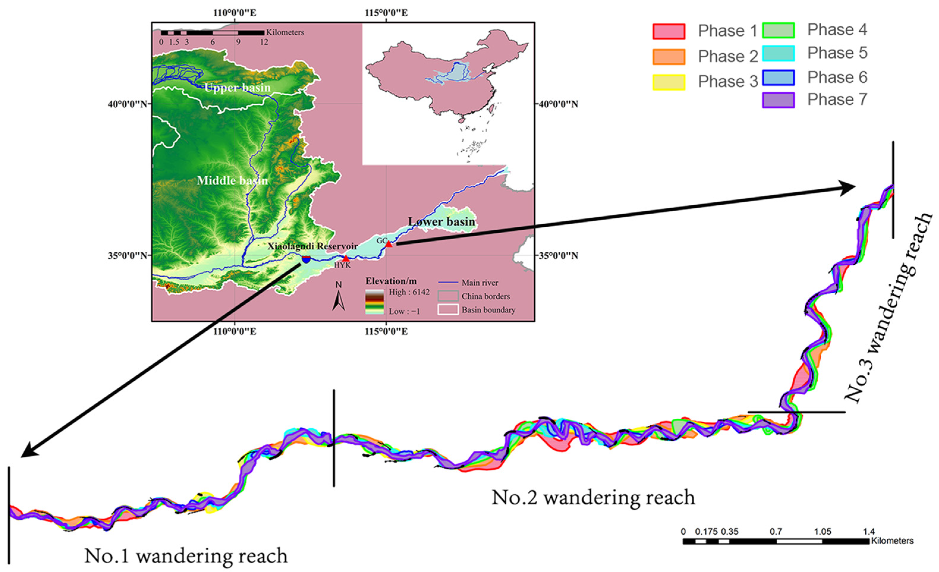
2.1. Study Area

The Yellow River is in the north of China, which has a full length of 5464 km and a basin area of about 795,000 km², as shown in Figure 1. Originating from the Bayankala Mountains on the Qinghai-Tibet Plateau in western China, the YR passes eastward through nine provinces in China and finally joins the Bohai Sea. Due to its vast size, each region of the YR varies markedly in terms of altitude, topography, and climate, with a wider range of temperature measurements. Annual precipitation in most parts of the YR basin ranges from 200 to 500 mm and is unevenly distributed throughout the year, most of which generally occur in the months of July and August. In addition, YR exhibits a unique phenomenon of different origins for water and sediment variations. The multi-year average natural runoff from 1956 to 2010 was 48.2 billion m³, of which about 62% and 28% were from upper and middle reaches, respectively. The average value of multi-year sediment transport over the same period was 1.6 billion tons, of which about 15% and 63% were from the upper and middle reaches, respectively.

According to the geomorphological characteristics of the Yellow River Basin (see Figure 1), the elevation of the upper, middle, and lower reaches gradually decreases. The lower Yellow River Basin completely presents a plain landform with flat land. The slope and velocity of the lower reach are clearly reduced, resulting in a large amount of sedimentation in the lower reaches. The wandering-pattern channel has a high degree of instability as the loose soil on both banks makes it susceptible to erosion and widening, leaving a wide but shallow transverse section. In addition, the scattered flow of water carries large amounts of sediment and raises the bed of the river due to deposition, creating the proverbial “hanging river”. Since the abrupt rise and fall of floods and large fluctuations of runoff, the main channel migration amplitude and rate are both high. The wandering-pattern reach has a wandering and varying river regime, probably causing the occurrence of transverse river and abnormal river bends, which are extremely difficult to regulate.

The enlarged section shown in Figure 1 represents the wandering reach, which is located at the downstream of the Xiaolangdi Reservoir to the Gaocun (GC) hydrometric station. The length of the wandering river reach is 299 km, the distance between embankments on both banks is 4.1–20.0 km, and its river slope is 0.172–0.256‰. To conduct the analysis, the wandering reach was divided into three parts according to the channel characteristics. The Taohuayu (THY) is located at the boundary between the middle and lower reaches of the YR; therefore, the river reach of the Xiaolangdi Reservoir to the THY is called the No.1 wandering reach. The Dongbatou (DBT) is located at the last big bend in the YR, the channel has a large change in the flow path, and the channel slope condition changes. With the DBT as the demarcation point, the THY to the DBT is called the No.2 wandering reach, and the No.3 wandering reach is from the DBT to the GC hydrometric station. The statistical information of channel characteristics of the wandering reaches of the YR is shown in

Table 1. Channel characteristics of the wandering reach of the Yellow River.

Wandering Reach	Length of Channel (km)	Width of Embankment (km)	Width of Channel (km)	Width of Beach Land (km)	Mean Grade of Slope (‰)
No.1	93	4.1–10.0	3.1–10.0	0.5–5.7	0.256
No.2	136	5.5–12.7	1.5–7.2	0.3–7.1	0.203
No.3	70	5.0–20.0	2.2–6.5	0.4–8.7	0.172

.

The Xiaolangdi Reservoir began to impound since October 1999, resulting in great changes in water and sediment conditions in the lower reaches. Due to the fact that river regime variations are very sensitive to water and sediment conditions, channel images in 1990 and 1995 were selected as the channel plane morphology of the first and second phases before the operation of the Xiaolangdi Reservoir. Since 2000, the channel images were taken as the channel plane morphology of the phase 3–7 every 5 years. By comparing the channel plane morphology of the seven periods, the dynamic changes in the channel in the wandering reach of the YR were analyzed.

2.2. Data Sources

There are two important hydrographic stations in the wandering reach of the YR, i.e., the Huayuankou (HYK) and GC stations, whose locations are marked as red triangles in Figure 1. To investigate the variations of water and sediment in the wandering reach of the YR, we collected the annual runoff and sediment transport data from the HYK and GC stations over the 64-year period 1952–2020. The HYK station is located at the downstream of the THY. The HYK station is generally recognized as the main station for observing runoff and sediment transport at the entrance of the LYR. The long-term observation recorded at the HYK station is sufficient to represent the features of the basin. The other station, i.e., the GC station, is located at the end of the wandering reach. The data of runoff and sediment observations from these two hydrometric stations are adequate to demonstrate the variation of the runoff and sediment transport. As the official sources of the YR data, the Yellow River Conservancy Commission (YRCC) can provide materials, such as the coordinate information about hydrometric stations as well as hydrological data, e.g., measured runoff, water depth, and velocity. In addition, it is strict with the reliability (quality) of these data. Therefore, the data issued by the YRCC were adopted in this study.

Digital elevation model of YR was acquired by processing the radar image data obtained by the Shuttle Radar Topography Mission, with the spatial resolution precision of 250 m. The datasets of Joint Research Center Monthly Water History (V1.1) with relatively high spatial resolution and long-time span were adopted, while the water boundary data of LYR from 1990 to 2015 were obtained using the Google Earth Engine. In addition, the water boundary data of LYR in 2020 were obtained using the Google Earth Pro software.

For the wandering reach of the YR, only when the channel-forming discharge (5000 m³/s) was achieved/sustained over a period of time, the river regime would be changed. The width of the regulation river is provided according to the channel-forming discharge; e.g., it is often determined as 0.8–1 km according to the state of river regime.

3. Methods

3.1. Trend Testing and Turning Point Identification

Annual runoff and sediment transport data were collected for two hydrometric stations from 1952 to 2020, then the trends for long-term time series were analyzed, and finally the years of turning points were tested. The principle of the non-parametric MK test was originally proposed by Mann [48] and Kendall [49] and was later refined and evolved into an equation by Yue and Pilon [50]. This method is now widely used to test for trends in series; therefore, the sample does not have to conform to any distributional regularity and is not disturbed by small outliers. Consequently, the method is applicable to type and rank variables, features relatively simple calculations, and can objectively identify the variation trend of data series. The time-series data $(X_1,X_2,\dots ,X_n)$ consist of n independent random variables. With $i,j\le n,$ and $i-j$, the distribution of $X_i$ and $X_j$ is different. The calculation of the testing statistic S is as follows [51]:

$$S={\displaystyle \sum _{i=1}^{n-1}{\displaystyle \sum _{j=i+1}^n\mathrm{sgn}\left(X_j-X_i\right)}}$$

(1)

where $X_i$ and $X_j$ are the observation values corresponding to the ith and jth epochs, and $i<j$, with $\mathrm{sgn}\left(a\right)$ as the sign function [52]:

$$\mathrm{sgn}\left(X_j-X_i\right)=\left\{\begin{array}{cc}{1}^{}\hfill & \left(X_j-X_i\right)>0\hfill \\ 0^{}\hfill & \left(X_j-X_i\right)=0\hfill \\ -1^{}\hfill & \left(X_j-X_i\right)<0\hfill \end{array}\right\}$$

(2)

When $n\ge 8$, the statistic S is basically in line with normal distribution. Without considering that the series has data points of equivalent values, its mean value $E\left(S\right)=0$. The variance formula is also shown as follows [53]:

$$\mathrm{var}\left(S\right)=\frac{n(n-1)(2n+5)-{\displaystyle \sum _{p=1}^g{t}_p\left(t_p-1\right)\left(2t_p+5\right)}}{18}$$

(3)

where g is the number of groups, and $t_p$ is the number of elements in every group. The standardized testing statistic Z is calculated as follows [54]:

$$Z=\left\{\begin{array}{cc}{\frac{S-1}{\sqrt{\mathrm{var}\left(S\right)}}}^{}\hfill & S>0\hfill \\ 0^{}\hfill & S=0\hfill \\ {\frac{S+1}{\sqrt{\mathrm{var}\left(S\right)}}}^{}& S<0\hfill \end{array}\right\}$$

(4)

Under the provided confidence level $\alpha$, Z exhibits normal distribution, with the time-series data showing a distinct ascending or descending trend. The positive values of Z indicate ascending trends, while the negative values indicate descending trends. When the absolute value of Z is no less than 1.645, 1.96, and 2.576, these denote the fact that the significance tests with the confidence levels of 90%, 95%, and 99%, respectively, are passed [55]. The gradient $\beta$ is used to measure the degree of trend:

$$\beta =median{\left(\frac{X_j-X_i}{j-i}\right)}^{}{{}^{}}^{}{{}^{}}^{}{}^{}\forall 1<i<j<n$$

(5)

where median (X) indicates the middle value, and the positive and negative values of $\beta$ indicate an ascending trend and a descending trend, respectively.

In a turning point test, $S_k$ indicates the accumulative number of the jth sample in the series $\left(X_1,X_2,\dots X_n\right)$ with $X_j>X_i\left(1\le i\le j\right)$. The definition of the statistic $S_k$ is listed as follows [56]:

$$S_k={{\displaystyle \sum _{j=1}^k{r}_j,}}^{}{r}_j={\{\begin{array}{cc}{1}^{}\hfill & X_j>X_i\hfill \\ 0^{}\hfill & X_j\le X_i\hfill \end{array}}^{}{}^{}\left(i=1,2,\dots ,j;k=1,2,\dots ,n\right)$$

(6)

Under the assumption of a random and independent time series, the mean value and variance of $S_k$ are expressed as:

$$E\left(S_k\right)={\frac{k(k-1)}{4}}^{}{{}^{}}^{}1<k<n$$

(7)

$$\mathrm{var}\left(S_k\right)={\frac{k(k-1)(2k+5)}{72}}^{}{{}^{}}^{}1<k<n$$

(8)

In the above equations, $S_k$ is standardized as [57]:

$$U{F}_k=\frac{S_k-E\left(S_k\right)}{\sqrt{\mathrm{var}\left(S_k\right)}}$$

(9)

where $U{F}_1=0$ and it indicates that the series has evident trend variation when $\left|U{F}_k\right|>\left|U_{\alpha }\right|$. When all the $U{F}_k$ are connected to form a curve, the reverse series $U{B}_k$ is obtained by setting $U{B}_k=-U{F}_k$ [58]. When the point of intersection between the two curves $U{F}_k$ and $U{B}_k$ is located inside the critical line of the confidence interval, it represents the fact that the moment corresponding to the point of intersection is the time for the beginning of turning.

3.2. Bank Line Variation

End Point Rate (EPR), representing the variation rate of the distance between both bank lines of a river in a certain period, can be directly used for the statistical analysis on the distance between both bank lines of a river. It is currently one of the most widely used methods in bank line change studies. In general, this method sets a baseline along the trend of a bank line at first, then the vertical lines of the equally spaced sampling points on the baseline to the bank line were sectional lines. It calculates corresponding variations based on the points of intersection between the sectional lines and the bank line. In this study, EPR was used to calculate the bank line variations of adjacent bank lines of each phase. The EPR of the south and north banks of the wandering reach of the YR with different patterns was respectively calculated and compared, and then the bank line variations were directly obtained based on the calculation results. The calculation formula of EPR is as follows [59]:

$$EP{R}_{\left(i,j\right)}=\frac{d_j-d_i}{\Delta T_{\left(j,i\right)}}$$

(10)

where $EP{R}_{\left(i,j\right)}$ is the variation rate at the end of the bank line along the tangent line between the ith and jth periods, $d_n$ is the distance between the bank line along the tangent line and the baseline in the nth stage, and $\Delta T_{\left(j,i\right)}$ is the value of the difference in years of the bank line between the ith and jth epochs.

The areas between the lines of the south and north banks over different periods are defined as the river surface area, which exhibits the state of deposition or erosion on the flood land by the river during the bank line variation process. Below is the formula for the calculation of the continuous variation rate $\left(\gamma {,}^{}{}^{}\%y{r}^{-1}\right)$ of the river surface area between one period and another [60]:

$$\gamma =\frac{\ln \left(A_j/A_i\right)}{\Delta T_{\left(j,i\right)}}$$

(11)

where $A_i$ and $A_j$ are the river surface areas at the ith and jth moments, respectively.

3.3. Theoretical Equations of the River Regulation Lines

Curved flow path is the most stable. Arc and tangent lines can be used to describe the river flow path by the mathematical methods. Based on the characteristics of conics, the piecewise equations of several types are proposed, which provide the theoretical basis for the rapid establishment of the river regulation lines flow path theory equation. The regulation lines of a river are generally two parallel curves; to facilitate the theoretical equation of the river regulation lines, this section takes the center line as the research object and provides the theoretical equation of the center line. Then, with the center line as the baseline, the points with equidistant of the center line are selected as the vertical line of the center line on both sides, and the length of the vertical line is half of the width of the river. Therefore, the two parallel river regulation lines can be obtained.

3.3.1. Equations of the Parabola

The flow path connecting two bend sections is called a transition reach. The parabola is an axially symmetric image with the maximum curvature at the vertex, and then the trajectory extends indefinitely to both ends of the opening direction and the curvature becomes progressively smaller [61]. After the parabolas with different opening directions are connected, they resemble a river flow path. In this section, the parabola is used to describe the center line of the river regulation lines.

As shown in Figure 2, a tangent line is developed through the vertex of the parabola. The direction of the tangent line is the horizontal axis and the vertical line of the tangent line is the vertical axis. Then, the two lines are translated to the intersection of the two adjacent parabolas, and the intersection is set as the origin.

The relationship between amplitude (2P) and span (2T) can be obtained from the property of parabola as follows:

$$\frac{2T}{2P}=\frac{2\sin \alpha }{1-\cos \alpha }$$

(12)

where 2P represents the amplitude of the center line, 2T denotes the span of the center line, and α refers to the angle of initiation, which is the angle between the tangent line of the parabola and the horizontal axis.

According to the parabolic general equation, the expression of the center line in Figure 1 can be written as follows [62]:

$$\{\begin{array}{cc}y=-\frac{4P}{T^2}{x}^2+\frac{4P}{T}{x}^{}{{}^{}}^{}{{}^{}}^{}{{}^{}}^{}{{}^{}}^{}{{}^{}}^{}{{}^{}}^{}{{}^{}}^{}{{}^{}}^{}{{}^{}}^{}\hfill & \left(0<x\le T\right)\hfill \\ y=\frac{4P}{T^2}{\left(x-T\right)}^2-\frac{4P}{T}{\left(x-T\right)}^{}{{}^{}}^{}{{}^{}}^{}{}^{}\hfill & \left(T<x\le 2T\right)\hfill \end{array}$$

(13)

The general equation is further derived as follows:

$$y={\left(-1\right)}^n\frac{4P}{T^2}{\left[x-\left(n-1\right)T\right]}^2+{\left(-1\right)}^{n+1}\frac{4P}{T}{\left[x-\left(n-1\right)T\right]}^{}{{}^{}}^{}{}^{}\left(\left(n-1\right)T<x\le nT\right)$$

(14)

where n is the number of river bends, and n is a positive integer.

The equations for the river regulation lines expressed as the parabolas are as follows:

$$\{\begin{array}{l}y={\left(-1\right)}^n\frac{4P}{T^2}{\left[x-\left(n-1\right)T\right]}^2+{\left(-1\right)}^{n+1}\frac{4P}{T}\left[x-\left(n-1\right)T\right]+\frac{B}{2}\\ y={\left(-1\right)}^n\frac{4P}{T^2}{\left[x-\left(n-1\right)T\right]}^2+{\left(-1\right)}^{n+1}\frac{4P}{T}\left[x-\left(n-1\right)T\right]-\frac{B}{2}\end{array}$$

(15)

where B refers to the width of regulating river.

In summary, the parabolic equations are simple in form and obtaining parameters is simple, we only need to obtain any two parameters of amplitude, span, and angle of initiation. From the graph of the parabola, the theoretical equations are more suitable for the river reach in which the amplitude is short, the river bend is curved, and the transition reach is short.

3.3.2. Equations of the Circular Arcs and Tangent Lines

The parabolic equations proposed in Section 3.3.1 can be found when the amplitudes of the two bends are wide and the transition reach tends to be straight. Therefore, it is herein considered to describe the bend reach with the circular arc line and the transition reach with the straight line, in order that the function can better fit the flow path. As a result, this section uses the circular arcs and the tangent lines of the circular arcs to construct the circular arcs and tangent lines equation in order to describe the center line.

As shown in Figure 3, the midpoint of the transition reach is considered as the origin of the coordinates, the amplitude direction as the vertical axis, and the vertical line through the origin as the horizontal axis.

From the properties of the circle, the following can be obtained [63]:

$$\phi =2\alpha$$

(16)

$$R=\frac{l}{2\sin \alpha }$$

(17)

$$k=\tan \alpha$$

(18)

where $\phi$ and R are the center angle and the radius of the circle, respectively, L denotes the length of the transition reach, l represents the chord length, and k is the slope of the tangent line of the circular arcs.

According to the general expression form of a circle, the equations of the center line shown in Figure 3 are:

$$\{\begin{array}{cc}y=k{x}^{}\hfill & \left(-\frac{L\cos \alpha }{2}<x\le \frac{L\cos \alpha }{2}\right)\hfill \\ y=\sqrt{R^2-{\left(x-\frac{L\cos \alpha +l}{2}\right)}^2}+\frac{L\sin \alpha }{2}-R\cos {\alpha }^{}{{}^{}}^{}\hfill & \left(\frac{L\cos \alpha }{2}<x\le \frac{L\cos \alpha }{2}+l\right)\hfill \end{array}$$

(19)

The river regulation left side bank line expressed as the theoretical equations of circular arcs and tangent lines are as follows:

$$\{\begin{array}{cc}y=kx+{\frac{B}{2}}^{}\hfill & \left(-\frac{L\cos \alpha }{2}<x\le \frac{L\cos \alpha }{2}\right)\hfill \\ y=\sqrt{R^2-{\left(x-\frac{L\cos \alpha +l}{2}\right)}^2}+\frac{L\sin \alpha }{2}-R\cos \alpha +{\frac{B}{2}}^{}\hfill & \left(\frac{L\cos \alpha }{2}<x\le \frac{L\cos \alpha }{2}+l\right)\hfill \end{array}$$

(20)

The river regulation right side bank line expressed as the theoretical equations of circular arcs and tangent lines are as follows:

$$\{\begin{array}{cc}y=kx-{\frac{B}{2}}^{}\hfill & \left(-\frac{L\cos \alpha }{2}<x\le \frac{L\cos \alpha }{2}\right)\hfill \\ y=\sqrt{R^2-{\left(x-\frac{L\cos \alpha +l}{2}\right)}^2}+\frac{L\sin \alpha }{2}-R\cos \alpha -{\frac{B}{2}}^{}\hfill & \left(\frac{L\cos \alpha }{2}<x\le \frac{L\cos \alpha }{2}+l\right)\hfill \end{array}$$

(21)

It can be seen from the line shown in Figure 3 that the theoretical equations of the circular arcs and tangent lines are applicable to the river bend which is curved, and the curvature of the connection between the bend and the transition reach changes slowly.

3.3.3. Equations of the Elliptical Arcs and Tangent Lines

With the gradual improvement of the training works, it can be found that the new construction of the training works extends upward and downstream on the original basis, the project becomes increasingly gentle, and the curvature of constrained river regimes decreases at the bend of the river. In this paper, the elliptic arcs whose curvature changes everywhere are used to describe the river bend. Therefore, this section presents the theoretical equations of the elliptical arcs and tangent lines.

The bend reach is represented by an elliptic arc, the straight line of the transition section is the tangent line connecting the two bend sections, and the distance between the two focal points of the ellipse is the chord length of the training work or the stable bend. Herein, we set the length of the semi-minor axis of the ellipse as the width of the regulating river.

The coordinate system is established with the extension line of the semi-major axis of the ellipse as the horizontal axis and the extension line of the semi-minor axis as the vertical axis, as shown in Figure 4.

The coordinates of two focal points of the ellipse are F(−c, 0) and F′(c, 0), respectively. According to the basic properties of ellipse, the following can be obtained [64]:

$$a^2=b^2+c^2$$

(22)

Let point P (x₀, y₀) be any point on the elliptical arc. According to the properties of the ellipse, the tangent equation at P can be obtained as follows:

$$y=y_0-\frac{b^2{x}_0}{a^2{y}_0}\left(x-x_0\right)$$

(23)

$$-\frac{b^2{x}_0}{a^2{y}_0}=\tan \alpha$$

(24)

where a is the semi-major axis length of the ellipse, and b is the semi-minor axis length of the ellipse. The coordinates of P can be obtained by combining Equation (24) with the basic equation of ellipse.

According to the general expression form of the ellipse, the equations of the center line shown in Figure 4 are:

$$\{\begin{array}{cc}y=y_0-\frac{b^2{x}_0}{a^2{y}_0}{\left(x-x_0\right)}^{}\hfill & \left(x_0-\frac{L}{2\sin \alpha }<x\le x_0\right)\hfill \\ y=b{\sqrt{1-\frac{x^2}{a^2}}}^{}\hfill & \left(x_0<x\le x_0+2\left|x_0\right|\right)\hfill \end{array}$$

(25)

The river regulation left side bank line expressed as the theoretical equations of the elliptical arcs and tangent lines are as follows:

$$\{\begin{array}{cc}y=y_0-\frac{b^2{x}_0}{a^2{y}_0}\left(x-x_0\right)+{\frac{B}{2}}^{}\hfill & \left(x_0-\frac{L}{2\sin \alpha }<x\le x_0\right)\hfill \\ y=b\sqrt{1-\frac{x^2}{a^2}}+{\frac{B}{2}}^{}\hfill & \left(x_0<x\le x_0+2\left|x_0\right|\right)\hfill \end{array}$$

(26)

The river regulation right side bank line expressed as the theoretical equations of the elliptical arcs and tangent lines are as follows:

$$\{\begin{array}{cc}y=y_0-\frac{b^2{x}_0}{a^2{y}_0}\left(x-x_0\right)-{\frac{B}{2}}^{}\hfill & \left(x_0-\frac{L}{2\sin \alpha }<x\le x_0\right)\hfill \\ y=b\sqrt{1-\frac{x^2}{a^2}}-{\frac{B}{2}}^{}\hfill & \left(x_0<x\le x_0+2\left|x_0\right|\right)\hfill \end{array}$$

(27)

It can be seen from Figure 4 that the elliptical arcs and tangent lines equation of the river regulation line are applicable to the flow path with a large area close to the training work at the bend, the chord length of the bend reach is long, and the curvature changes quickly at the bend and the transition reach.

3.3.4. Equations of the Elliptical Arcs, Curvature Circular Arcs, and Tangent Lines

In this section, situated between the equations of the circular arcs/tangent lines and the equation of the elliptical arcs/tangent lines, the equations of the elliptical/curvature circular arcs and tangent lines have been proposed to describe the center of the regulation line.

The establishment of the coordinate system is similar to Section 3.3.3, as shown in Figure 5.

Suppose point P (x₀, y₀) is any point on the ellipse. Then, an outer circle of an ellipse is made with a semi-major axis as the radius, a perpendicular line is made through point P to the x-axis, and the circle intersects with point Q (x₀, y₁). The two points of P and Q share the same x-coordinate; this ∠QOF is the eccentric angle of P. According to the general expression of ellipse, the ordinate y₀ of P is expressed as follows [65]:

$$y_0=b\sqrt{1-\frac{x_0^2}{a^2}}$$

(28)

According to the general expression of circle, the ordinate y₁ of Q can be determined using:

$$y_1=\sqrt{a^2-x_0^2}$$

(29)

The eccentric angle θ of P can be obtained using the above relation. The curvature at P is:

$$k=\frac{ab}{{\left(a^2{\sin }^2\theta +b^2{\cos }^2\theta \right)}^{3/2}}$$

(30)

where k refers to the curvature at P, and the radius of the curvature circle R is the reciprocal of the curvature. The equation of the curvature circle can be expressed as:

$${\left(x-\frac{\left(a^2-b^2\right){\cos }^3\theta }{a}\right)}^2+{\left(y+\frac{\left(a^2-b^2\right){\sin }^3\theta }{b}\right)}^2=\frac{{\left(a^2{\sin }^2\theta +b^2{\cos }^2\theta \right)}^3}{a^2{b}^2}$$

(31)

Suppose the slope of the tangent line at point M (x_m, y_m) on the curvature circle is:

$$\tan \alpha =\frac{\left(a^2-b^2\right)\frac{{\cos }^3\theta }{a}-x_m}{\sqrt{{\left(1/k\right)}^2-{\left[x_m-\left(a^2-b^2\right)\frac{{\cos }^3\theta }{a}\right]}^2}}$$

(32)

The x-coordinate x_m of M can be obtained using Equation (32), and the y-coordinate y_m of M can be obtained from the curvature circle equation. By substituting M into the general formal equation of the tangent line, the intercept c of the line can be obtained as follows:

$$c=y_m-\frac{\left(a^2-b^2\right)\frac{{\cos }^3\theta }{a}-x_m}{\sqrt{{\left(1/k\right)}^2-{\left[x_m-\left(a^2-b^2\right)\frac{{\cos }^3\theta }{a}\right]}^2}}{x}_m$$

(33)

After sorting out the above formulas, the center line equation of the river regulation line shown in Figure 5 can be written as follows:

$$\{\begin{array}{cc}y=x\tan \alpha +c^{}\hfill & \left(-\frac{c}{\tan \alpha }<x\le x_m\right)\hfill \\ y=\sqrt{\frac{{\left(a^2{\sin }^2\theta +b^2{\cos }^2\theta \right)}^3}{a^2{b}^2}-{\left(x-\frac{\left(a^2-b^2\right){\cos }^3\theta }{a}\right)}^2}-{\frac{\left(a^2-b^2\right){\sin }^3\theta }{b}}^{}\hfill & \left(x_m<x\le x_0\right)\hfill \\ y=b{\sqrt{1-\frac{x^2}{a^2}}}^{}\hfill & \left(x_0<x\le x_0+2\left|x_0\right|\right)\hfill \end{array}$$

(34)

The river regulation left side bank line expressed as the theoretical equations of the elliptical arcs, curvature circular arcs, and tangent lines are as follows:

$$\{\begin{array}{cc}y=x\tan \alpha +c+{\frac{B}{2}}^{}\hfill & \left(-\frac{c}{\tan \alpha }<x\le x_m\right)\hfill \\ y=\sqrt{\frac{{\left(a^2{\sin }^2\theta +b^2{\cos }^2\theta \right)}^3}{a^2{b}^2}-{\left(x-\frac{\left(a^2-b^2\right){\cos }^3\theta }{a}\right)}^2}-\frac{\left(a^2-b^2\right){\sin }^3\theta }{b}+{\frac{B}{2}}^{}\hfill & \left(x_m<x\le x_0\right)\hfill \\ y=b\sqrt{1-\frac{x^2}{a^2}}+{\frac{B}{2}}^{}\hfill & \left(x_0<x\le x_0+2\left|x_0\right|\right)\hfill \end{array}$$

(35)

The river regulation right side bank line expressed as the theoretical equations of the elliptical arcs, curvature circular arcs, and tangent lines are as follows:

$$\{\begin{array}{cc}y=x\tan \alpha +c-{\frac{B}{2}}^{}\hfill & \left(-\frac{c}{\tan \alpha }<x\le x_m\right)\hfill \\ y=\sqrt{\frac{{\left(a^2{\sin }^2\theta +b^2{\cos }^2\theta \right)}^3}{a^2{b}^2}-{\left(x-\frac{\left(a^2-b^2\right){\cos }^3\theta }{a}\right)}^2}-\frac{\left(a^2-b^2\right){\sin }^3\theta }{b}-{\frac{B}{2}}^{}\hfill & \left(x_m<x\le x_0\right)\hfill \\ y=b\sqrt{1-\frac{x^2}{a^2}}-{\frac{B}{2}}^{}\hfill & \left(x_0<x\le x_0+2\left|x_0\right|\right)\hfill \end{array}$$

(36)

Based on the equations of the circular arcs and tangent lines, the elliptic arc is added to describe the gentle shape at the top of the river bend. Their theoretical equations have wider ranges of application and are more adaptive to describing the river section. In addition, the river regime at the top of bend is close to the project and then a smooth transition is made to the straight reach.

4. Results

4.1. Investigation on Variation Trends of Runoff and Sediment Transport

The variation trends of the annual runoff and sediment transport of the wandering reach of YR from 1952 to 2020 are shown in Figure 6. The height of each dot represents the anomaly value of runoff, and their sizes denote the values of sediment transport. Based on the multi-year observation data at the two hydrometric stations, it was found that the annual runoff and sediment transport over the period 1952−2020 exhibited a reducing trend. Among the runoff observed at the two stations, the annual runoff in 1997 was the lowest. Specifically, the values obtained at the HYK and GC hydrometric stations are 14.26 and 10.34 billion m³ yr⁻¹, respectively. In addition, the annual sediment transport in 2016 observed at the two stations was the lowest, their respective values are 6 and 18 million. The MK trend test revealed a decreasing trend in annual runoff and sediment transport at the two stations from 1952 to 2020. Among them, the HYK hydrometric station had an evidently decreasing trend of the annual runoff with p < 0.01 after 1992, and an evidently decreasing trend of the annual sediment transport with p < 0.01 after 1991. Similarly, the other station, GC, had an evidently decreasing trend of the annual runoff with p < 0.01 after 1991, and an evidently decreasing trend of the annual sediment transport with p < 0.01 after 1989.

The turning points of the annual runoff and sediment transport at the two stations are represented as the red and yellow dots in Figure 6 and they were calculated using the two-tailed test to observe the points of intersection between UF and UB. The red dots represent the years of the annual runoff turning points, while the yellow dots represent the years of the annual sediment transport turning points. The years of the annual runoff turning points for the HYK and GC hydrometric stations are 1979 and 1978, respectively, while the years of the annual sediment transport turning points for these stations are 1995 and 1992, respectively. Drastic changes in water and sediment conditions will inevitably lead to dramatic river regimes movement.

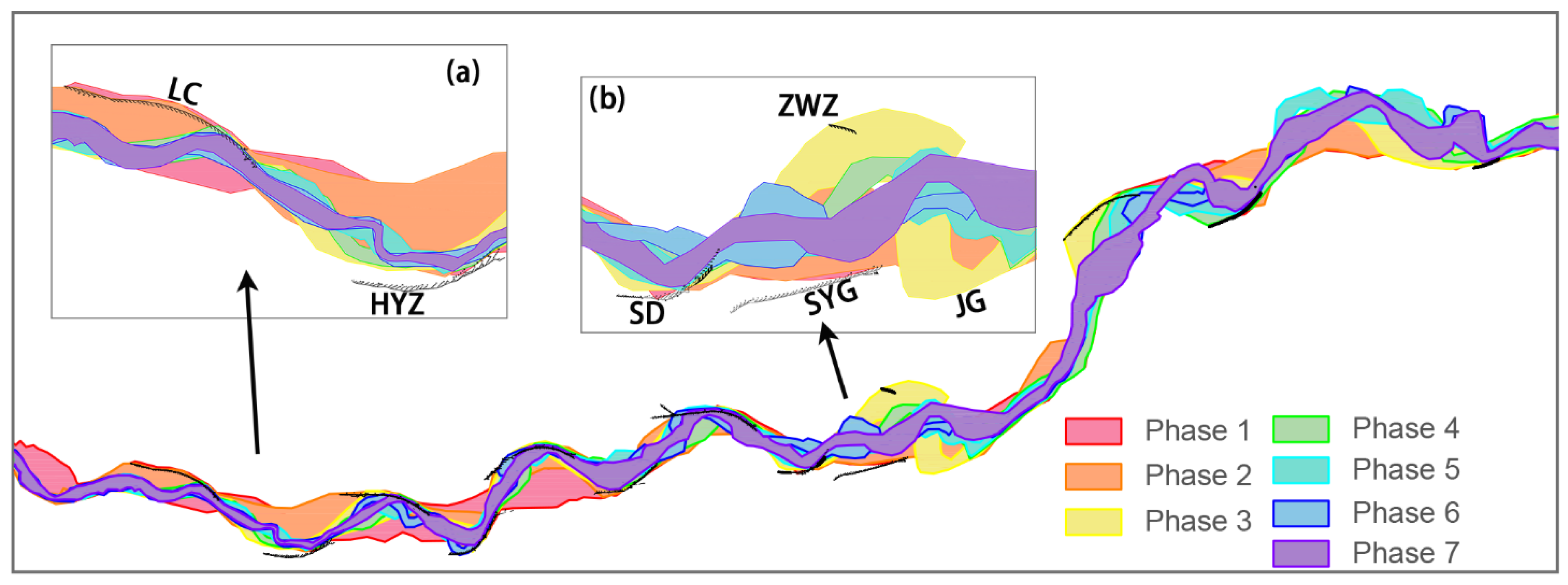
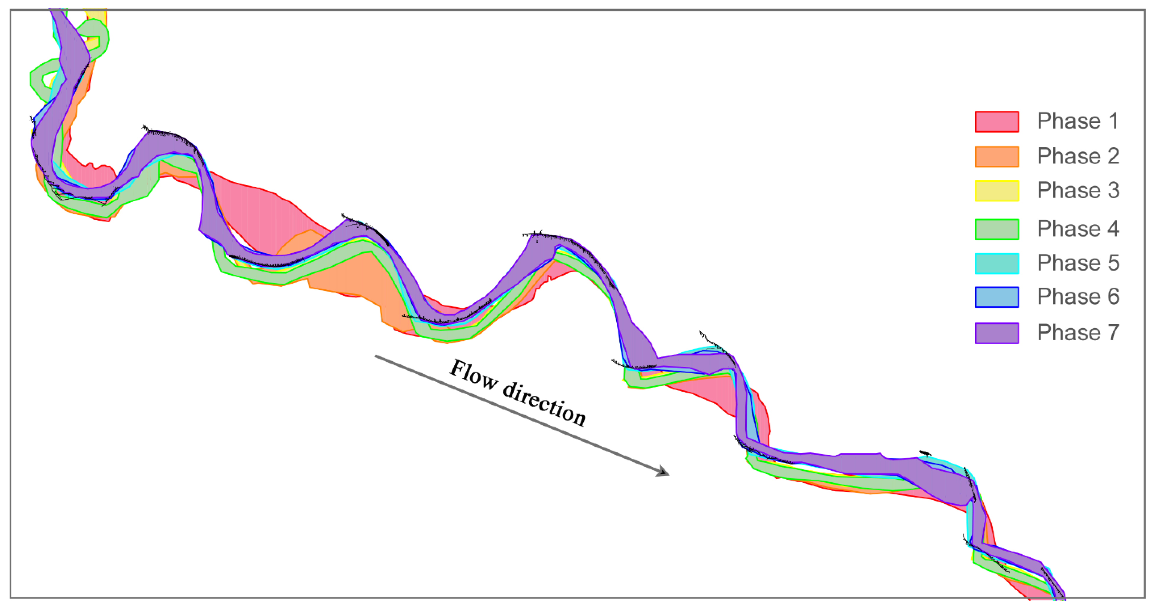
4.2. Analysis of River Regimes Evolution in Wandering Reach of Yellow River

According to the phase division stated in Section 2.1, a total of seven phases of channel plane morphology of the wandering reach of the YR from 1990 to 2020 were shown in Figure 1. The seven phases of channel plane morphology were stacked together for comparison. At the current stage, the 190-km-long mainstream in the wandering reach has already been stabilized, while the regime of the other 109-km-long stream is still changing significantly. Most of the river regimes changed dramatically before (i.e., phases 1 and 2) and within 10 years of operational use (i.e., phases 3 and 4) of the Xiaolangdi Reservoir. While after phase 5, the river regimes start to become relatively stable.

The bends in the wandering reach of the YR are usually named by the nearby village. To introduce the characteristics of the typical river reaches, the names of these bends are shown in Figure 7 and Figure 8, such as the Zhangwangzhuang (ZWZ), Shayugou (SYG), and Baohezhai (BHZ). Figure 7 shows the historical evolution of the No.1 wandering reach. As the connecting section between the middle and lower reaches, it generally belongs to the transitional reach from the valley to the alluvial plain, and the river regimes changed dramatically. Figure 7a depicts the river regimes of the reach from Lucun (LC) to Huayuanzhen (HYZ), the amount of water of which has decreased significantly after phase 4, and some small bends have also appeared. As shown in Figure 7b, prior to the operation of the Xiaolangdi Reservoir, the main flow path was wide and unstable in the reach from Shendi (SD) to Jingou (JG). After the operation of the Xiaolangdi Reservoir, although the mainstream still continuously oscillates, its oscillation amplitude has clearly decreased. After phase 5, the mainstream of the other reaches basically moved along the flow path, and the variations were not very clear.

The plane morphology variations of the No.2 wandering reach are shown in Figure 8. The flow paths of phases 1, 2, 3, and 4 are arbitrary and unstable. The river regimes vary frequently with many deformed bends. As shown in Figure 8a, the training works of the reach from Laotianan (LTA) to HYK have lost control of the river regimes since phase 5, during which its water and sediment volumes have been considerably decreased. With the operation of the Xiaolangdi Reservoir and the further improvement of the training works, the whole river regimes developed in a favorable direction from phase 5. Although the mainstream is still swinging, the swing amplitude decreases at the same time. In addition, as shown in Figure 8b, there are still some partial river reaches, such as the Sanguanmiao (SGM) to the Dazhangzhuang (DZZ), where the river regimes were not controlled and the main stream is still swinging greatly.

Figure 9 shows the plane morphology variations in the No.3 wandering reach. In general, the river regime is relatively regular, simple, and basically stable. Especially after the operation of the Xiaolangdi Reservoir, it remains stable and the partial river regimes possess a varying trend in accordance with the water level.

According to the wandering reach of the YR and its phase division provided in Section 2.1, the river bank line drawn in Section 4.2 and the method in Section 3.2 are used to calculate the river channel change index. The EPR of bank line variation and the continuous rate of water surface area are the most common used indicators.

The change rates of the north and south bank line in the adjacent periods of the three river reaches were calculated respectively, as shown in Figure 10. Figure 10a shows that the north bank line is changed actively from 1990 to 1995, and the most active reach was the No.3 wandering reach. Compared with phase 1, the EPR value of phase 2 is increased by 2.16 km/yr. The changes in the south bank line are shown in Figure 10b. Prior to the operation of the Xiaolangdi Reservoir, the bank line of the river changed significantly in all periods, and the maximum EPR appeared in the No.1 wandering reach. Compared with phase 2, the EPR value of phase 3 increased by 1.61 km/yr.

In general, the absolute values of EPR in the No.1 and No.3 wandering reaches were larger before the operation of the Xiaolangdi Reservoir, while the values in the adjacent two phases were smaller after phase 4. There is no clear rule in the absolute value of EPR in the two adjacent phases of the No.2 wandering reach, indicating that the reach still has a certain oscillation, which also corresponds to the river regimes evolution as shown in Figure 8.

The calculation results of the continuous change rate of the water surface area in the two adjacent phases are shown in Figure 11. The rate changed relatively fast before the construction of the Xiaolangdi Reservoir. The water surface area changes the fastest in the No.3 wandering reach from phase 2 to phase 3, and the water surface area in phase 3 decreases by 9.96% compared with phase 2. After phase 4, the water surface area of the No.3 wandering reach was relatively stable.

In general, the evolution of river regimes in the wandering reach of the YR is known to be quite complicated. Over the period from 1990 to 2005, the swing of the main flow path was large. Although the river regime became relatively stable after the year 2010, some partial river regimes still changed significantly. It is necessary to build training works according to the current river regimes to better constrain the development of the river regimes; therefore, it is very important to be able to quickly and efficiently plan the river regulation lines.

4.3. Verification of the Theoretical Equations of the River Regulation Lines

Based on the theoretical equation of four kinds of river regulation lines and their applicable river regimes proposed in Section 3.3, several typical river reaches or bends in the wandering reach of the YR are used for verification in this section. According to the location of the project and the river regimes in 2020, the Shuangjing (SJ)–Shenzhuang (SZ) reach, DBT bend, Gubaizui (GBZ) bend, and Dayulan (DYL) bend are selected to verify the theoretical equations of the river regulation lines of the parabola, the circular arcs and tangent lines, the elliptical arcs and tangent lines, and the elliptical arcs, curvature arcs, and tangent lines, respectively.

4.3.1. The SJ–SZ Reach

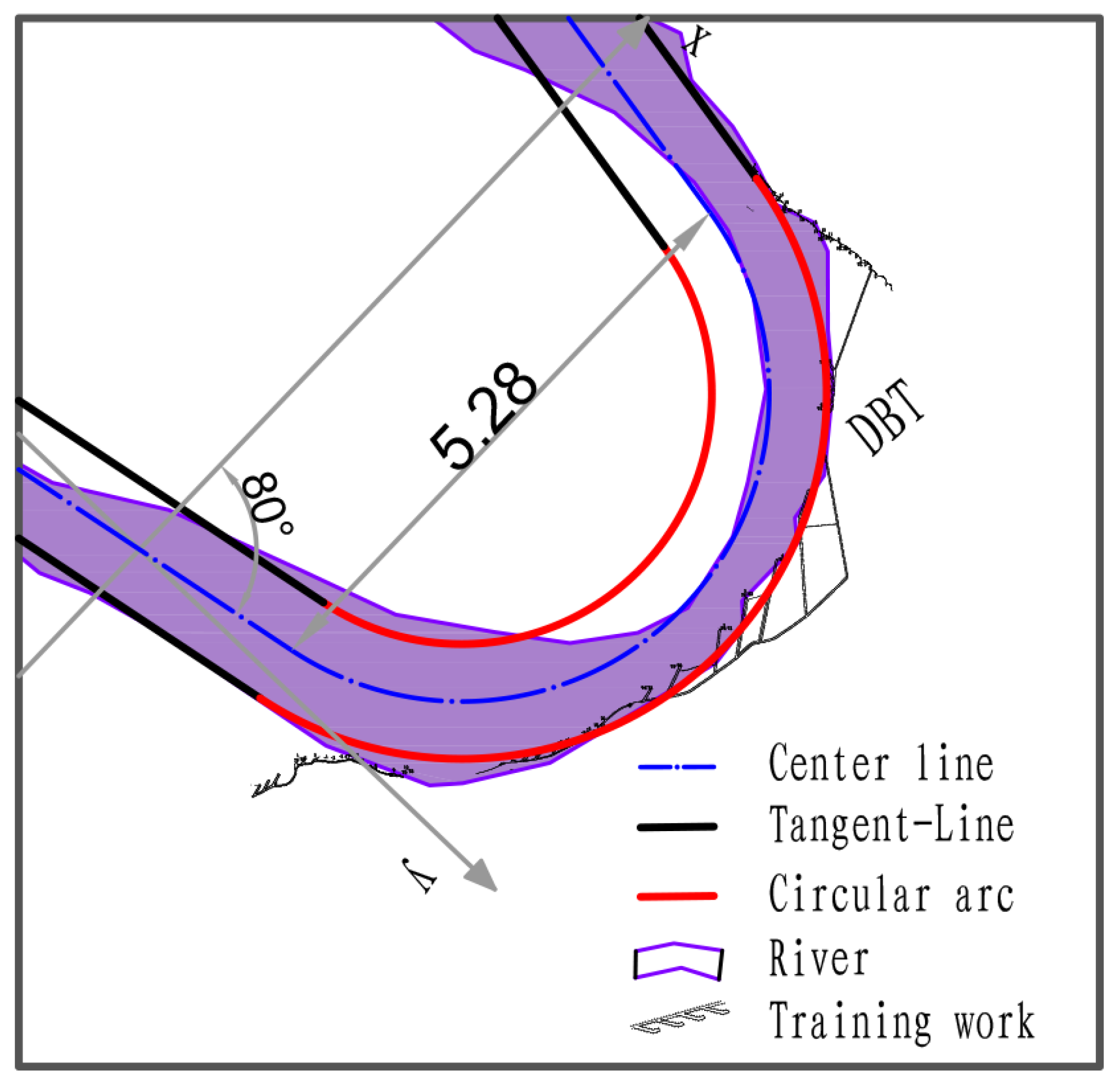
The theoretical equations of the river regulation lines of the parabola are verified using the SJ–SZ reach. The SJ–SZ reach is in the No.2 wandering reach, and the width of the regulating river is set as 0.8 km according to the river regimes development over the years. The amplitude measured in the SJ–SZ reach is 3.64 km; namely, 2P is 2.84 km, the span is 12.46 km, and the coordinate system is established as shown in Figure 12.

According to Equation (15), the left bank equation of parabolic river regulation lines in the SJ–SZ reach can be written as follows:

$$\{\begin{array}{ll}y=-0.146343097x^2+0.911717496x+{0.4}^{}{{}^{}}^{}{{}^{}}^{}{{}^{}}^{}{{}^{}}^{}{{}^{}}^{}{{}^{}}^{}{}^{}& \left(0<x\le 6.23\right)\\ y=0.146343097{\left(x-6.23\right)}^2-0.911717496x+{6.08}^{}{{}^{}}^{}& \left(6.23<x\le 12.46\right)\end{array}$$

(37)

The right bank equation of parabolic river regulation lines in the SJ–SZ reach can be written as follows:

$$\{\begin{array}{cc}y=-0.146343097x^2+0.911717496x-{0.4}^{}\hfill & \left(0<x\le 6.23\right)\hfill \\ y=0.146343097{\left(x-6.23\right)}^2-0.911717496x+{5.28}^{}\hfill & \left(6.23<x\le 12.46\right)\hfill \end{array}$$

(38)

As can be seen from Figure 12, the curve can better plan river regulation lines in SJ–SZ reach. By measuring the span and amplitude, the center line equation can be obtained quickly. The parabolic equation is applicable to the curved river channel which can satisfy the central symmetry and the amplitude is short. The parabolic equations are applicable to the curved channel connecting two boughs which can satisfy the central symmetry and have a short amplitude. In the natural river, especially the wandering river reach, only a few river reaches can be quickly obtained by the parabolic equation.

4.3.2. The DBT Bend

DBT is the last U-turn in the YR. It has dangerous terrain, and its curvature is large. It can be used to verify the applicability of the circular arcs and tangent lines equation. The midpoint connection of the length of the upstream and downstream transition reaches of DBT bend is the x-axis, the measurement of the angle of initiation is 80°, the measurement engineering chord parallel to the x-axis is 5.28 km, and the width of the regulating river is set as 1 km. The coordinate system is established as shown in Figure 13.

According to Equation (20), the left bank equation of the circular arcs and tangent lines river regulation lines in the DBT bend can be written as follows:

$$\{\begin{array}{cc}y=5.67128182x+{0.5}^{}\hfill & \left(-0.300431754<x\le 0.300431754\right)\hfill \\ y=\sqrt{{2.680726255}^2-{\left(x-2.940431754\right)}^2}+{1.738329914}^{}\hfill & \left(0.300431754<x\le 5.580431754\right)\hfill \\ y=-5.67128182x+{33.85203429}^{}\hfill & \left(5.580431754<x\le 6.181295261\right)\hfill \end{array}$$

(39)

According to Equation (21), the right bank equation of the circular arcs and tangent lines river regulation lines in the DBT bend can be written as follows:

$$\{\begin{array}{cc}y=5.67128182x-{0.5}^{}\hfill & \left(-0.300431754<x\le 0.300431754\right)\hfill \\ y=\sqrt{{2.680726255}^2-{\left(x-2.940431754\right)}^2}+{0.738329914}^{}\hfill & \left(0.300431754<x\le 5.580431754\right)\hfill \\ y=-5.67128182x+{32.85203429}^{}\hfill & \left(5.580431754<x\le 6.181295261\right)\hfill \end{array}$$

(40)

The circular arcs and tangent lines equation can be well adapted to the DBT bend. The continuous equations of the river regulation lines can be obtained by measuring the engineering chord length and the angle of initiation. In the river reach with a gentle curvature change, the circular arcs and tangent lines equation can well plan the future trend of river regime and the position of training works.

4.3.3. The GBZ bend

Some river bends are small, even close to the straight flow of the bend. If this bend is described by the circular arcs, the radius is significantly large and it is difficult to determine the center of the circle. The GBZ bend, as a representative of a bend with low curvature, is used in this section to verify the elliptical arcs and tangent lines equation. The measured chord length of the bend is 4.2 km, the width of the modified river is 1 km, the angle of initiation in the upstream and downstream of the bend is 21 and 18°, and the vertical line across the apex of the bend is the y-axis. The coordinate system is shown in Figure 14.

According to Equation (26), the left bank equation of the elliptical arcs and tangent lines river regulation lines in the GBZ bend can be written as follows:

$$\{\begin{array}{cc}y=2.904210878x+{7.328640044}^{}\hfill & \left(-2.401713367<x\le -2.300865289\right)\hfill \\ y=\sqrt{1-\frac{x^2}{5.41}}+{0.5}^{}\hfill & \left(-2.300865289<x\le 2.291624738\right)\hfill \\ y=-2.475086853x+{6.343111943}^{}\hfill & \left(2.291624738<x\le 2.429916193\right)\hfill \end{array}$$

(41)

According to Equation (27), the right bank equation of the elliptical arcs and tangent lines river regulation lines in the GBZ bend can be written as follows:

$$\{\begin{array}{cc}y=2.904210878x+{6.328640044}^{}\hfill & \left(-2.401713367<x\le -2.300865289\right)\hfill \\ y=\sqrt{1-\frac{x^2}{5.41}}-{0.5}^{}\hfill & \left(-2.300865289<x\le 2.291624738\right)\hfill \\ y=-2.475086853x+{5.343111943}^{}\hfill & \left(2.291624738<x\le 2.429916193\right)\hfill \end{array}$$

(42)

By measuring the chord length and the angle of initiation of the bend, the elliptical arcs and tangent lines equation of the bend can be provided, and the flow path of the river regulation lines can clearly show the future trend of the river regime. The slight river bend is more unstable than the curved reach, and its river regime changes more violently than the curved reach, which is the key point of river regulation in the future. By determining the river regulation lines, the layout and position of the future training works can be planned. With the evolution of river regimes, it is instructive to use the elliptical arcs and tangent lines equation to describe the river regimes at the present stage.

4.3.4. The DYL Bend

At present, most of the bends in the wandering reach of the YR are regular with little variation, and the top of the bends is relatively flat with the continuous extension of the training works. The curvature from the transition reach to the bend changes quickly, which is a common problem. The elliptical arcs, curvature arcs, and tangent lines can be connected to describe the existing river regimes and training works. Taking the DYL bend as an example, the coordinate system as shown in Figure 15 is established, where the chord length of the river bend is 3.89 km and the width of the regulated river is 1 km.

According to Equation (35), the left bank equation of the elliptical arcs, curvature arcs, and tangent lines river regulation lines in the DBT bend can be written as follows:

$$\{\begin{array}{cc}y=1.191753593x+{3.498093872}^{}\hfill & \left(-3.9564<x\le -2.063193962\right)\hfill \\ y=\sqrt{1.302957018-{\left(x+1.188776119\right)}^2}+{0.103686636}^{}\hfill & \left(-2.063193962<x\le -1.9308\right)\hfill \\ y=\sqrt{1-\frac{x^2}{4.79119841}}+{0.5}^{}\hfill & \left(-1.9308<x\le 1.3381\right)\hfill \\ y=\sqrt{8.01943404-{\left(x-0.395688942\right)}^2}-{1.379062742}^{}\hfill & \left(1.3381<x\le 2.565019962\right)\hfill \\ y=-1.191753593x+{3.498093872}^{}\hfill & \left(2.565019962<x\le 3.9564\right)\hfill \end{array}$$

(43)

According to Equation (36), the right bank equation of the elliptical arcs, curvature arcs, and tangent lines river regulation lines in the DBT bend can be written as follows:

$$\{\begin{array}{cc}y=1.191753593x+{2.498093872}^{}\hfill & \left(-3.9564<x\le -2.063193962\right)\hfill \\ y=\sqrt{1.302957018-{\left(x+1.188776119\right)}^2}-{0.896313364}^{}\hfill & \left(-2.063193962<x\le -1.9308\right)\hfill \\ y=\sqrt{1-\frac{x^2}{4.79119841}}-{0.5}^{}\hfill & \left(-1.9308<x\le 1.3381\right)\hfill \\ y=\sqrt{8.01943404-{\left(x-0.395688942\right)}^2}-{0.379062742}^{}\hfill & \left(1.3381<x\le 2.565019962\right)\hfill \\ y=-1.191753593x+{2.498093872}^{}\hfill & \left(2.565019962<x\le 3.9564\right)\hfill \end{array}$$

(44)

Using the chord length and the angle of initiation, the river regulation lines at the DYL bend can be provided, which can better describe the river regimes development, fit the training works, and guide the layout of the future project. The elliptical arcs, curvature arcs, and tangent lines river regulation lines equations have a wide range of application, the parameters are easy to obtain, and the line changes are flexible.

To realize the suitability of the new river regulation line to the flow path and the existing training works, the deviation distances between the center line of the river regulation line and the river regime are calculated. The length of the above four river reaches is about 10 km. The deviation distance between the two lines is recorded every 100 m along the x-axis and y-axis, and these data are collected for analysis (

Table 2. Measurements of deviation distance between the center line of the river and river regulation lines.

Item of Statistical Analysis	Direction	SJ–SZ Reach	DBT Bend	GBZ Bend	DYL Bend
Mean Value (km)	x-axis	0.20	0.18	0.14	0.19
	y-axis	0.30	0.31	0.40	0.14
Standard Deviation (km)	x-axis	0.155	0.142	0.085	0.111
	y-axis	0.299	0.316	0.210	0.113

). As can be seen from Table 2, the mean deviation distance of the four verified reaches is less than 0.5 km, indicating that the river regulation line deviates slightly from the flow path, and the flow path can be easily adjusted to the direction of the river regulation line under certain conditions. The standard deviation of the four verified reaches is also small, with the maximum value of 0.316 km. The measures of dispersion of the data are small and concentrated, there is no deviation distance significantly greater/less than the average value in the dataset. By analyzing the data of the deviation distance between the center line of the river regulation line and flow path, it is believed that the river regulation line matches the current river regime well, and it can better guide the future river regime development.

In summary, it is verified by the typical reaches or bends of the wandering reach of the YR, which shows that the theoretical equations of the four types of curves proposed in Section 3.3 can be used to plan river regulation lines according to different river regimes and existing training works. Among them, the parabola and the elliptical arcs and tangent lines equations have fewer target river reaches, and the circular arcs and tangent lines and the elliptical arcs, curvature arcs, and tangent lines equations are more suitable for most wandering river reaches.

In terms of parameters, the parameters required by each method are relatively easy to obtain. By establishing equations, the flow curve of the river regulation can be quickly obtained, which provides a theoretical basis for the planning and design of the river regulation line, and provides a basis for the layout of the training works.

5. Discussion

This section selects the Xindianji (XDJ)–Zhouying (ZY)–Laojuntang (LJT) reach in the wandering reach of the YR, which is located in the No.1 wandering reach in Figure 1. The feature of this reach is that the length of the transition section between XDJ and ZY is longer, and the curvature changes quickly in LJT. Moreover, there is an island braided at ZY, which divides the flow road into two parts. In this section, the bend curvature of XDJ changes evenly, the bending degree and length of the project are moderate. The connection between the transition reach and the bend in ZY is rapid, where the bend is relatively gentle and the chord length of the project is long. The curvature of the bend at LJT changes quickly and the chord length of the project is short. Section 4.3 uses the single river bend to verify the river regulation lines equations. In this section, the continuous and representative river reach will be used to apply the proposed theoretical equations and compare it with the traditional river regulation lines design method.

5.1. Planning and Design of River Regulation Lines Using the Traditional Method

The river regimes and projects layout in the flood season in 2020 are used to analyze the planning and design of the river regulation lines of the XDJ–ZY–LJT reach. At present, the traditional method is used to design the river regulation lines as shown in Figure 16.

As can be seen from Figure 16, the circular arcs and tangent lines connection are adopted in all the planning of traditional river regulation lines. For the long bend, a circular arc with a larger radius or the tangent of two circular arcs with different radii is used to describe it. By observing the river regulation lines at the XDJ, it can be found that, to connect the lines at the upstream transition section, the arc of the XDJ cannot accurately describe the river regime and project position; therefore, there is a large deviation. The lines in the transition section of the lower XDJ reach are relatively matched with the river regimes, but the planned path is not close to the river regimes and the project at the upper ZY reach. In particular, the river regulation path guides the river flow directly to the island. In terms of the current flow of the LYR, it is difficult to reach the channel-forming discharge for a period of time under the water and sediment conditions in operation; therefore, it is difficult to change the flow path by eroding the island. The bend of the river at LJT is curved, and the circular arc can well describe the project location to guide the future development direction of the river. In summary, the river regulation lines at present still need to be further perfected and improved.

To test whether the traditional method can describe the river regulation lines better, the traditional method is still used to improve the river regulation lines. As mentioned in the above paragraph, the ZY bend, where the river regulation lines have a big problem, is still designed by increasing the radius and tangent of two circular arcs, as shown in Figure 17.

After increasing the radius of the circular arc at the upper ZY reach to match the flow path and the position of the training works, the river regulation line in the transition section, as the tangent line of the circular arc, is difficult to match the actual flow path due to the large radius of the circular arc, as shown in Figure 17a. As far as possible, the arc should be close to the river regime and the project at the bend, close to the river regime at the transition section, and well connected to the bend at XDJ. The planned river regulation lines are shown in Figure 17b. Compared with the current flow path, the modified lines are relatively close to the river regime and the project at ZY bend, but there is still a gap in the degree of matching the river regime and the project. To ensure the tangent between the arcs, the center of the arc must be on the radius or extension line of the contact arc, which also restricts the arc at the upper ZY reach to match the river regimes and the project by increasing the radius.

5.2. Comparison of the New and Traditional Methods

According to the equations of the river regulation lines proposed in Section 3.3, the XDJ–ZY–LJT reach is redesigned. Elliptical and curvature arcs equations are used for the XDJ and XDJ bends, while circular arcs equations are used for the LJT bend. The new river regulation lines are shown in Figure 18.

The theoretical equations proposed in Section 3.3 were used for planning and design. It can be seen from Figure 18a that the river regulation lines at the XDJ bend can closely fit the existing project and river regime. In ZY bend, the newly designed lines avoided the flow path on the right side of the island and planned the flow path to pass through the left side. The elliptical arc was used to extend the distance between the two circular arcs, which better described the river regime and the project at the ZY bend. The river regimes of the LJT are only restricted by the second half of the project, the new river regulation lines are similar to the current lines, but closer to the project.

Figure 18b shows the comparison between the new and the original river regulation lines. It can be found that the new lines are more adaptive to the current river regime and the layout of training works. First, select any point at the center line of the river as the intersection to construct a vertical line. The constructed perpendicular line is intersected with the new and traditional regulation lines as well as the training works. Specifically, the fitting performance of these new and traditional regulation lines can be evaluated by comparing their distances with the river training works. The distances between the new river regulation lines and the position of the training works at the XDJ, ZY, and LJT are 0.07, 0.52, and 0.12 km, respectively. The distances between the traditional river regulation lines and the position of the training works at the XDJ, ZY, and LJT are 0.45, 0.75, and 0.13 km, respectively. It can be clearly found that the new river regulation lines are closer to the training works and river regimes, which can guide flow directions of stream path in future scenarios.

Moreover, Figure 18b depicts the fact that when using these new methods to plan the river regulation lines in adjacent river bends, each of them can be connected tangently in the transition reach. Therefore, these new methods have the ability to provide some useful clues and guidance for future river development and the following training works construction.

The center line of the traditional/new river regulation line and flow path was compared and analyzed (see

Table 3. Measurements of deviation distance between the center line of the traditional and new river regulation lines.

Item of Statistical Analysis	Direction	Traditional River Regulation Lines	New River Regulation Lines
Mean Value (km)	x-axis	0.72	0.50
	y-axis	0.65	0.49
Standard Deviation (km)	x-axis	0.548	0.525
	y-axis	0.310	0.263

). The total length of the reach for verification in Figure 18 is 23.5 km. Since there are three bends in this reach, a separate coordinate axis was established for the analysis of deviation distance, as shown in Figure 18b. The values and analysis methods are the same as those stated in Section 4.3. It can be seen from Table 3 that the statistical analysis results of x-axis and y-axis indicate that the new river regulation line is superior to the traditional one. The mean value of the deviation distance and the dispersion degree of the dataset were smaller. The new river regulation line has the smallest deviation distance along the y-axis (0.49 km), and the dataset is also the most concentrated (0.263 km). These results further corroborate that the planning of the new river regulation line is easier in order to make the river regime adjust in this direction, and the new river regulation line is closer to the existing training work. When the new training work is conducted according to the river regulation line, the regulation line can make the new training work connect with the existing training work in a more appropriate way.

6. Conclusions

In this study, the theoretical equations of river regulation lines applicable to different river reaches were established. These equations can be used to plan and design the river regulation lines quickly and effectively, thus to provide clues and insights for the river regime development and subsequent training works layout position in future scenarios.

Taking the wandering reach of the Yellow River as an example, it can be divided into three reaches according to channel characteristics, i.e., No.1, No.2, and No.3 wandering reaches. The drastic changes in the annual runoff and sediment transport of the wandering reach of the Yellow River from 1952 to 2020 inevitably lead to dramatic river regimes movement. By analyzing the river regime evolution process over the period from 1990 to 2020, it was found that the wandering channel of the Yellow River has gradually become obedient after the implementation of the training works and the change in water and sediment conditions after the construction of the Xiaolangdi Reservoir. In addition, it was discovered that there is no longer a large channel change, but some frequent small amplitude swings. It is still of great necessity to rely on the training works constraint to further control the river regime change. Furthermore, the effective time period of the river regulation lines is greatly shortened due to the frequent changes in the river regimes and the need to update the design of the new river regulation lines according to the new river regime and training works. The calculation of the river change index also indicated that the river change was drastic and relatively weakened before and after the operation of the Xiaolangdi Reservoir, respectively. In view of the above situations, it is important to establish the effective theoretical equations for the river regulation lines.

Four types of theoretical equations of the river regulation lines for different river regimes and the training works position were proposed. The required parameters of each theoretical equation are easy to obtain. Among these equations, the parabola equations are suitable for the small river bend with short amplitude and the curved river with short transition reach. The equations of circular arcs and tangent lines are applicable to the river bend which is curved and the situation when the curvature of the connection between the bend and transition reach changes slowly. The elliptical arcs and tangent lines equations are applicable to the flow path of the large area close to the training works at the bend, the chord length of the bend reach is long, and the curvature changes quickly at the transition reach. The equations of the elliptical arcs, curvature circular arcs, and tangent lines have a wider range of applications, which are more suitable to describe the river reach where the river regimes at the top of bend are close to the project and then gently transition to the straight reach.

Finally, the theoretical equations of the river regulation lines were verified using different reaches and bends, the results of which were proved to be promising. By comparing the new methods with the original ones, it was also found that the planning and design of the new river regulation lines are significantly faster and more convenient. In general, the methods proposed in this study not only have the potential to effectively describe the river regimes and the training works position, but can also provide some useful references for guiding the future river regimes development and the subsequent training works layout in future scenarios.

References

1. Plink-Björklund, P. Stacked fluvial and tide-dominated estuarine deposits in high-frequency (fourth-order) sequences of the Eocene Central Basin, Spitsbergen. Sedimentology 2005, 52, 391–428. [Google Scholar] [CrossRef]
2. Lunt, I.A.; Bridge, J.S.; Tye, R.S. A quantitative, three-dimensional depositional model of gravelly braided rivers. Sedimentology 2004, 51, 377–414. [Google Scholar] [CrossRef]
3. Schumm, S.A.; Dumont, J.; Holbrook, J. Active Tectonics and Alluvial Rivers; Cambridge University Press: Cambridge, UK, 2000; pp. 270–276. [Google Scholar]
4. Chen, W.; Xu, Q.; Ma, Y.; Zhang, X. Palaeochannels on the north china plain: Palaeoriver geomorphology. Geomorphology 1996, 18, 37–45. [Google Scholar] [CrossRef]
5. Herbert, G. Sequence stratigraphic analysis of early and middle Triassic alluvial and estuarine fades in the Sydney Basin, Australia. Aust. J. Earth Sci. 1997, 44, 125–143. [Google Scholar] [CrossRef]
6. Žibret, G.; Gosar, M. Calculation of the mercury accumulation in the Idrijca River alluvial plain sediments. Sci. Total. Environ. 2006, 368, 291–297. [Google Scholar] [CrossRef]
7. Latrubesse, E.M.; Franzinelli, E. The Holocene alluvial plain of the middle Amazon River, Brazil. Geomorphology 2002, 44, 241–257. [Google Scholar] [CrossRef]
8. Wang, S.; Yan, Y.; Li, Y. Spatial and temporal variations of suspended sediment deposition in the alluvial reach of the upper Yellow River from 1952 to 2007. Catena 2012, 92, 30–37. [Google Scholar] [CrossRef]
9. Wang, S.; Fu, B.; Piao, S.; Lü, Y.; Ciais, P.; Feng, X.; Wang, Y. Reduced sediment transport in the Yellow River due to anthropogenic changes. Nat. Geosci. 2016, 9, 38–41. [Google Scholar] [CrossRef]
10. Schumm, S.A. Patterns of alluvial rivers. Annu. Rev. Earth Planet. Sci. 1985, 13, 5–27. [Google Scholar] [CrossRef]
11. Nanson, G.C.; Knighton, A. Anabranching rivers: Their cause, character and classification. Earth Surf. Process. Landf. 1994, 21, 217–239. [Google Scholar] [CrossRef]
12. Carling, P.; Jansen, J.; Meshkova, L. Multichannel rivers: Their definition and classification. Earth Surf. Process. Landf. 2013, 39, 26–37. [Google Scholar] [CrossRef]
13. Liu, Y.; Wang, Y.; Jiang, E. Stability index for the planview morphology of alluvial rivers and a case study of the Lower Yellow River. Geomorphology 2021, 389, 107853. [Google Scholar] [CrossRef]
14. Kondolf, G.M.; Gao, Y.; Annandale, G.W.; Morris, G.L.; Jiang, E.; Zhang, J.; Cao, Y.; Carling, P.; Fu, K.; Guo, Q.; et al. Sustainable sediment management in reservoirs and regulated rivers: Experiences from five continents. Earths Future 2014, 2, 256–280. [Google Scholar] [CrossRef]
15. Tu, Q.H.; An, C.; Qing, Z.; Zhang, S.; Zhang, H. Riverbed evolution of the lower Yellow River and water and sediment regulation by Xiaolangdi Reservoir. River Sediment. Theory Appl. 1999, 24, 855–860. [Google Scholar]
16. Yin, S.; Gao, G.; Ran, L.; Lu, X.; Fu, B. Spatiotemporal Variations of Sediment Discharge and In-Reach Sediment Budget in the Yellow River from the Headwater to the Delta. Water Resour. Res. 2021, 57, e2021WR030130. [Google Scholar] [CrossRef]
17. Milly, P.C.D.; Dunne, K.A.; Vecchia, A.V. Global pattern of trends in streamflow and water availability in a changing climate. Nature 2005, 438, 347–350. [Google Scholar] [CrossRef]
18. Oki, T.; Kanae, S. Global Hydrological Cycles and World Water Resources. Science 2006, 313, 1068–1072. [Google Scholar] [CrossRef] [Green Version]
19. Li, Y.; Chang, J.; Tu, H.; Wang, X. Impact of the Sanmenxia and Xiaolangdi Reservoirs Operation on the Hydrologic Regime of the Lower Yellow River. J. Hydrol. Eng. 2016, 21, 06015015. [Google Scholar] [CrossRef]
20. Maren, D.; Ming, Y.; Zheng, B. Predicting the morphodynamic response of silt-laden rivers to water and sediment release from reservoirs: Lower yellow river, China. J. Hydrol. Eng. 2010, 137, 900–999. [Google Scholar]
21. Ma, L.; Zhang, H.; Zhong, D. Design of regulation line based on check and balance mechanism. J. Hydrol. Eng. 2016, 47, 1315–1321. [Google Scholar]
22. Zhang, H.W.; Zhang, J.; Zhong, D.; Bu, H. Regulation strategies for wandering reaches of Lower Yellow River. J. Hydraul. Eng. 2011, 42, 8–13. [Google Scholar]
23. Guo, Y.; Li, C.; Wang, C.; Xu, J.; Jin, C.; Yang, S. Sediment routing and anthropogenic impact in the Huanghe River catchment, China: An investigation using Nd isotopes of river sediments. Water Resour. Res. 2021, 57, e2020WR028444. [Google Scholar] [CrossRef]
24. Su, T.; Huang, H.Q.; Carling, P.A.; Yu, G.; Nanson, G.C. Channel-Form Adjustment of an Alluvial River Under Hydrodynamic and Eco-Geomorphologic Controls: Insights from Applying Equilibrium Theory Governing Alluvial Channel Flow. Water Resour. Res. 2021, 57, e2020WR029174. [Google Scholar] [CrossRef]
25. Wu, X.; Wang, H.; Bi, N.; Xu, J.; Nittrouer, J.; Yang, Z. Impact of artificial floods on the quantity and grain size of riv-er-borne sediment: A case study of a dam regulation scheme in the Yellow River catchment. Water Resour. Res. 2021, 57, e2021WR029581. [Google Scholar] [CrossRef]
26. Yang, Z.; Wang, H.; Saito, Y.; Milliman, J.D.; Xu, K.; Qiao, S.; Shi, G. Dam impacts on the Changjiang (Yangtze) River sediment discharge to the sea: The past 55 years and after the Three Gorges Dam. Water Resour. Res. 2006, 42, W04407. [Google Scholar] [CrossRef]
27. Xu, J.; Ma, Y. Response of the hydrological regime of the Yellow River to the changing monsoon intensity and human activity. Hydrol. Sci. J. 2009, 54, 90–100. [Google Scholar] [CrossRef]
28. Jiang, C.; Xiong, L.; Guo, S.; Xia, J.; Xu, C.-Y. A process-based insight into nonstationarity of the probability distribution of annual runoff. Water Resour. Res. 2017, 53, 4214–4235. [Google Scholar] [CrossRef] [Green Version]
29. Cong, Z.; Yang, D.; Gao, B.; Yang, H.; Hu, H. Hydrological trend analysis in the Yellow River basin using a distributed hydro-logical model. Water Resour. Res. 2009, 45, 7. [Google Scholar] [CrossRef]
30. Yan, J.; Liang, B.; Cao, H.; Zhang, Y.H. BP Model Used for Calculating the High Efficient Sediment-Transport Water Volume in the Lower Yellow River. Adv. Mater. Res. 2011, 225, 1345–1349. [Google Scholar] [CrossRef]
31. Pan, B.; Han, M.; Wei, F.; Tian, L.X.; Liu, Y.T.; Li, Y.; Wang, M. Analysis of the Variation Characteristics of Runoff and Sediment in the Yellow River Within 70 Years. Water Resour. 2021, 48, 676–689. [Google Scholar] [CrossRef]
32. Wang, H.; Sun, F. Variability of annual sediment load and runoff in the Yellow River for the last 100 years (1919–2018). Sci. Total. Environ. 2020, 758, 143715. [Google Scholar] [CrossRef] [PubMed]
33. Li, W.; Fu, X.; Wu, W.; Wu, B. Study on runoff and sediment process variation in the lower yellow river. J. Hydroelectr. Eng. 2014, 33, 108–113. [Google Scholar] [CrossRef]
34. Zhang, X.; Song, C.; Hu, D. Research on the periodic regularity of annual runoff in the Lower Yellow River. J. Water Clim. Chang. 2018, 10, 130–141. [Google Scholar] [CrossRef]
35. Gao, P.; Mu, X.-M.; Wang, F.; Li, R. Changes in streamflow and sediment discharge and the response to human activities in the middle reaches of the Yellow River. Hydrol. Earth Syst. Sci. 2011, 15, 1–10. [Google Scholar] [CrossRef]
36. Xu, J. Effect of human activities on overall trend of sedimentation in the lower yellow river, China. Environ. Manag. 2004, 33, 637–653. [Google Scholar]
37. Cavadias, G. Detection and modeling of the impact of climatic change on riverflows. In Engineering Risk in Natural Resources Management; Springer: Berlin/Heidelberg, Germany, 1994; pp. 207–218. [Google Scholar]
38. Pirani, F.J.; Najafi, M. Recent trends in individual and multivariate compound flood drivers in Canada’s coasts. Water Resour. Res. 2020, 56, e2020WR027785. [Google Scholar]
39. Wrzesinski, D.; Ptak, M. Water level changes in Polish lakes during 1976–2010. J. Geogr. Sci. 2016, 26, 83–101. [Google Scholar] [CrossRef] [Green Version]
40. Asfaw, A.; Simane, B.; Hassen, A.; Bantider, A. Variability and time series trend analysis of rainfall and temperature in northcentral Ethiopia: A case study in Woleka sub-basin. Weather. Clim. Extrem. 2018, 19, 29–41. [Google Scholar] [CrossRef]
41. Strohmenger, L.; Fovet, O.; Akkal-Corfini, N.; Dupas, R.; Durand, P.; Faucheux, M. Multitemporal relationships between the hydroclimate and exports of carbon, nitrogen, and phosphorus in a small agricultural watershed. Water Resour. Res. 2020, 56, e2019WR026323. [Google Scholar] [CrossRef]
42. Xu, K.; Milliman, J.D.; Xu, H. Temporal trend of precipitation and runoff in major Chinese Rivers since 1951. Glob. Planet. Chang. 2010, 73, 219–232. [Google Scholar] [CrossRef]
43. Kisi, O.; Haktanir, T.; Ardiclioglu, M.; Ozturk, O.; Yalcin, E.; Uludag, S. Adaptive neuro-fuzzy computing technique for sus-pended sediment estimation. Adv. Eng. Softw. 2009, 40, 438–444. [Google Scholar] [CrossRef]
44. Zhang, L.Z.; Wan, Q.; Huang, H. The Statistical Law of Regulation Parameters of the Meandering Channel in the Lower Yellow River. In Proceedings of the 4th International Yellow River Forum on Ecological Civilization and River Ethics V, Zhengzhou, China, 20–23 October 2009; pp. 198–201. [Google Scholar]
45. Li, Y.Q.; Wang, B.; Liu, Y. Research on Applicability of Lower Yellow River Training Works after Beginning of Xiaolangdi Reservoir Operation. In Proceedings of the 2012 International Conference on Modern Hydraulic Engineering, Nanjing, China, 9–11 March 2012; Volume 28, pp. 776–780. [Google Scholar]
46. Zhang, C.P.; Zhang, R.; Jiang, N.; Hu, T. Review on planned and revised alignments of channel regulation in the lower Weihe river. J. Sediment Res. 2009, 5, 47–51. [Google Scholar]
47. Wu, B.; Ma, J.; Zhang, B.; Ma, J. Morphological Response to River Training in the Lower Yellow River. In Proceedings of the 1st International Yellow River Forum on River Basin Management, Zhengzhou, China, 21–24 October 2003; Volume 2. [Google Scholar]
48. Mann, H.B. Nonparametric tests against trend. Econometrica 1945, 13, 245–259. [Google Scholar] [CrossRef]
49. Kendall, M.G. Rank Correlation Methods; Griffin: London, UK, 1975. [Google Scholar]
50. Yue, S.; Pilon, P. A comparison of the power of the t-test, Mann-Kendall and bootstrap tests for trend detection/Une comparaison de la puissance des tests t de Student, de Mann-Kendall et du bootstrap pour la détection de tendance. Hydrol. Sci. J. 2004, 49, 21–37. [Google Scholar] [CrossRef]
51. Hirsch, R.M.; Slack, J.R.; Smith, R.A. Techniques of trend analysis for monthly water-quality data. Water Resour. Res. 1981, 18, 107–121. [Google Scholar] [CrossRef] [Green Version]
52. Gan, T.Y. Finding Trends in Air Temperature and Precipitation for Canada and Northeastern United States. In Using Hydrometric Data to Detect and Monitor Climate Change; NHRI Workshop No. 8; National Hydrology Research Institute: Saskatoon, SK, Canada, 1992; pp. 57–78. [Google Scholar]
53. Hamed, K.H.; Raom, A.R. A modified Mann-Kendall trend test for autocorrelated data. J. Hydrol. 1998, 204, 182–196. [Google Scholar] [CrossRef]
54. Pour, S.H.; Abd Wahab, A.K.; Shahid, S. Spatial pattern of the unidirectional trends in thermal bioclimatic indicators in Iran. Sustainability 2019, 11, 2287. [Google Scholar] [CrossRef]
55. Alhaji, U.U.; Yusuf, A.S.; Edet, C.O.; Oche, C.O.; Agbo, E.P. Trend Analysis of Temperature in Gombe State Using Mann Kendall Trend Test. J. Sci. Res. Rep. 2018, 20, 1–9. [Google Scholar] [CrossRef]
56. Xing, L.; Huang, L.; Chi, G.; Yang, L.; Li, C.; Hou, X. A Dynamic Study of a Karst Spring Based on Wavelet Analysis and the Mann-Kendall Trend Test. Water 2018, 10, 698. [Google Scholar] [CrossRef] [Green Version]
57. Lv, X.; Zuo, Z.; Ni, Y.; Sun, J.; Wang, H. The effects of climate and catchment characteristic change on streamflow in a typical tributary of the Yellow River. Sci. Rep. 2019, 9, 1–10. [Google Scholar] [CrossRef] [Green Version]
58. Liang, K.; Liu, C.; Liu, X. Impacts of climate variability and human activity on streamflow decrease in a sediment con-centrated region in the Middle Yellow River. Stoch. Environ. Res. Risk Assess. 2013, 27, 1741–1749. [Google Scholar] [CrossRef]
59. Mukhopadhyay, A.; Mukherjee, S.; Mukherjee, S.; Ghosh, S.; Hazra, S.; Mitra, D. Automatic shoreline detection and future prediction: A case study on Puri Coast, Bay of Bengal, India. Eur. J. Remote Sens. 2012, 45, 201–213. [Google Scholar] [CrossRef]
60. Simonsen, L.; Gordon, D.M.; Stewart, F.M. Estimating the rate of plasmid transfer: An end-point method. Microbiology 1990, 136, 2319–2325. [Google Scholar] [CrossRef] [PubMed]
61. Avner, F. Partial Differential Equations of Parabolic Type; Courier Dover Publications: Mineola, NY, USA, 2008. [Google Scholar]
62. Bettina, R.; Richmond, T. How to recognize a parabola. Am. Math. Mon. 2009, 116, 910–922. [Google Scholar]
63. Kazimierz, J. Approximation of Smooth Planar Curves by Circular arc Splines. 2012. Available online: http://kaj.uniwersytetradom.pl/prace/Biarcs.pdf (accessed on 11 November 2022).
64. Qing, H.; Lin, F. Elliptic partial differential equations. Am. Math. Soc. 2011, 1, 147. [Google Scholar]
65. Mishra, R.B.; Nagireddy, S.R.; Bhattacharjee, S.; Hussain, A.M. Theoretical Modeling and Numerical Simulation of Elliptical Capacitive Pressure Microsensor. In Proceedings of the 2019 IEEE Conference on Modeling of Systems Circuits and Devices (MOS-AK India), Hyderabad, India, 25–27 February 2019; pp. 17–22. [Google Scholar]
Figure 1. Detailed information regarding the study area.
Sustainability 15 01965 g001
Figure 2. The center line described by the parabola.
Sustainability 15 01965 g002
Figure 3. The center line described by the circular arcs (red) and tangent lines (black).
Sustainability 15 01965 g003
Figure 4. The center line described by the elliptical arcs (red) and tangent lines (black). Note that the red solid lines are parts of the determined center line, and the red dashed lines represents the formation of the ellipses.
Sustainability 15 01965 g004
Figure 5. The center line described by the elliptical arcs (red), curvature circular arcs (blue), and tangent lines (black). Note that the dashed lines depict the formation of the elliptical and curvature circular arcs.
Sustainability 15 01965 g005
Figure 6. The variation trends of the annual runoff and sediment transport obtained at the Huayuankou (a) and Gaocun stations (b) over the period 1952–2020.
Sustainability 15 01965 g006
Figure 7. Superposition of river plane morphology over the period 1990−2020 of the No.1 wandering reach. The subfigure (a) denotes the river regimes of the reach from LC to HYZ; and the subfigure (b) illustrates some wide and unstable reaches.
Sustainability 15 01965 g007
Figure 8. Superposition of river plane morphology over the period 1990−2020 of the No.2 wandering reach. The subfigure (a) denotes the training works of the reach from LTA to HYK; and the subfigure (b) illustrates some partial river reaches.
Sustainability 15 01965 g008
Figure 9. Superposition of river plane morphology over the period 1990−2020 of the No.3 wandering reach.
Sustainability 15 01965 g009
Figure 10. The EPR of the adjacent two phases in the north (a) and south (b) bank lines of the wandering reach of the Yellow River.
Sustainability 15 01965 g010
Figure 11. The continuous variation rate of the water surface area of two adjacent phases.
Sustainability 15 01965 g011
Figure 12. The river regulation lines plan for the Shuangjing (SJ)–Shenzhuang (SZ) reach (1:100,000).
Sustainability 15 01965 g012
Figure 13. The river regulation lines plan for the Dongbatou (DBT) bend (1:100,000).
Sustainability 15 01965 g013
Figure 14. The river regulation lines plan for the Gubaizui (GBZ) bend (1:100,000).
Sustainability 15 01965 g014
Figure 15. The river regulation lines plan for the Dayulan (DYL) bend (1:100,000).
Sustainability 15 01965 g015
Figure 16. Planning and design of the river regulation lines at present in the XDJ–ZY–LJT reach.
Sustainability 15 01965 g016
Figure 17. The improved river regulation lines developed at the Xindianji (XDJ)-Zhouying (ZY) reach based on the traditional design method. Note that the subfigure (a) denotes the closest regulation lines to river regime, and the subfigure (b) represents the optimal regulation line.
Sustainability 15 01965 g017
Figure 18. Comparison between the regulation lines developed at the Xindianji (XDJ)-Zhouying (ZY)-Laojuntang (LJT) reach using the new and traditional methods. Note that the subfigure (a) denotes the regulation lines designed by the new method; the subfigure (b) shows the comparison results.
Sustainability 15 01965 g018