Article

Influence of Financial Support to Agriculture on Carbon Emission Intensity of the Industry

School of Economics, Anhui University, Hefei 230601, China
*
Author to whom correspondence should be addressed.
Sustainability 2023, 15(3), 2228; https://doi.org/10.3390/su15032228
Submission received: 7 December 2022 / Revised: 20 January 2023 / Accepted: 23 January 2023 / Published: 25 January 2023

Abstract

:
Financial support to agriculture is an important means by which to support agricultural development. While promoting agricultural economic growth, it also has an influence on the agricultural production environment. In order to explore the sustainable development of the agricultural economy, based on the provincial panel data of 31 provinces in China from 2000 to 2020, this paper uses Geoda software to construct a spatial distance weight matrix and uses Stata software to establish a spatial Durbin model of random effects, and analyzes the influence of the level of financial support to agriculture on the intensity of agricultural carbon emission (ACE). The results show that the support level has a significant spatial spillover effect, and that every 1% increase in the support level will increase the carbon emission (CE) intensity of the province by 0.1357% and the CE intensity of neighboring provinces by 0.0714%. Based on this, this paper puts forward suggestions that the structure of China’s financial support to agriculture needs to be further optimized, and that it is necessary to use such support to coordinate emission reduction.

1. Introduction

The massive release of greenhouse gasses makes the greenhouse effect more serious and causes huge damage to global climate. Carbon dioxide is an important part of the greenhouse gas, and reducing its emissions is the first priority to solve the problem of climate change. As a promoter and practitioner of addressing climate change, China has been actively contributing to environmental protection, and has repeatedly proposed to implement voluntary emission reductions.
Xia et al. proposed the use of panel data from 30 provinces and autonomous regions in mainland China (excluding Tibet) from 2006 to 2016 to conduct empirical research using the spatial Derbin model, and analyze the spatial impact of fiscal decentralization and environmental decentralization on regional carbon emissions from the perspective of official promotion pressure. The empirical study concluded that fiscal decentralization within and around the region would help to reduce carbon emissions [1]. Yuanhua Yang et al. also proposed that fiscal decentralization significantly curbs carbon emissions in the eastern region, aggravates carbon emissions in the western region, and has no significant impact on carbon emissions in the central region [2]. Agriculture is not only a huge carbon sink, but is also an important source of global greenhouse gas emissions. Moreover, good ecosystems can absorb nearly 80% of the greenhouse gasses caused by agriculture. According to survey data from the Food and Agriculture Organization of the United Nations (FAO), nearly one-third of the world’s annual anthropogenic greenhouse gas emissions (about 15 billion tons of CO2) are generated from agriculture. The essence of achieving carbon peaking and carbon neutrality is to promote the transformation of economic development to green and low carbon [3]. Global ACE has increased by 14% since the 1990s. According to forecasts, the world’s population will continue to rise in the next few decades. By 2050, the global population could reach 9 billion. Therefore, a large increase in food is required to ensure human survival needs. It can be seen that, in the future, reducing ACE is a major issue that needs to be globally solved. Since agriculture has a background of green ecology, promoting agricultural emission reduction and carbon sequestration is not only an important measure to implement the rural revitalization strategy, but is also the main way to deal with global climate change [4].
Some scholars from other countries and regions have found through research that agricultural finance can not only promote local agricultural development, but also have an influence on non-agricultural industries [5], and this effect has different results in different regions. Generally speaking, increasing financial support to agriculture in areas with better economic development will promote the development of the local economy, while increasing financial support to agriculture in areas with a highly regressive economy will hinder the development of the local economy. The reason for this is that regressive areas cannot reasonably and effectively distribute financial support to agriculture [6]. It is worth mentioning that the financial support proposed in this paper is mainly through the provision of financial support, such as supporting the use of more fertilizers or the introduction of better, environmentally friendly machines or technologies; in turn, leading to the scientific and effective control and reduction of agricultural carbon emissions. In the literature [7], the authors used the DEA method to determine that the comprehensive efficiency of financial support to agriculture in the western, central and eastern regions is increasing in turn; the scale efficiency of the central region is the highest, indicating that the scale of financial support to agriculture is more reasonable.
Research on ACE has mainly focused on two aspects: one to measure ACE, and the other to study the influence of other related factors on ACE. Regarding the calculation method of ACE, in the literature [8], the authors measured ACE in four dimensions: pesticides, chemical fertilizers, agricultural irrigation, and seed cultivation. In the literature [9], the authors calculated the agricultural greenhouse gasses produced by rice and livestock raising and considered that it is necessary to promote greenhouse gas emission reduction technologies. Some scholars studied ACE at a specifically small scale, such as livestock breeding [10] and energy consumption [11], and the index system constructed was relatively simple. In addition, indicators constructed by other scholars have been more comprehensive [12], basically covering the entire agricultural production sector. In recent years, environmental problems have become increasingly prominent, and many scholars have begun to study the influencing factors of ACE. For example, the increase in industrial agglomeration will increase the amount of agricultural net carbon effect [13], scientific and technological progress can have an inhibitory effect on ACE [14], and the level of urbanization has a positive influence on ACE in the province and a negative influence on ACE in neighboring provinces [15]. These studies have provided theoretical references for agricultural CE reduction.
This paper firstly explores the spatial effect of CE by using the relevant data from the website of the National Bureau of Statistics, “China Rural Statistical Yearbook” and “China Price Statistical Yearbook”. Then, this paper uses Geoda software to construct a spatial distance 0-1 matrix, and combines the spatial Durbin model to analyze the influence of the level of financial support to agriculture on the intensity of ACE, examining the overall effect and the decomposition effect. In addition, this paper establishes provincial panel data with agricultural CE intensity as the explained variable, the level of financial support to agriculture as the observation variable, and a number of factors related to agricultural production as the control variables. Finally, this paper conducts empirical analysis using Stata software to discuss the direction, size, and significance of the influence of financial support on ACE.

2. Relationship between Financial Support and Agricultural Carbon Emissions

Through a review of the literature, it is not difficult to determine that financial support has a direct impact on agricultural carbon emissions. This impact is manifested in the effective reduction of carbon emissions from agricultural production with increased financial support, such as the introduction of more advanced technical support and the use of more environmentally friendly fertilizers. From the perspective of the scale of financial support to agriculture, scholars have studied the influence of financial support on ACE. In the literature [16], the authors believed that the influence of the scale of fiscal expenditure on environmental quality is related to the degree of government democracy, and a society with a high degree of democracy can use financial support to agriculture to improve environmental quality. Many scholars have studied the relationship between financial support to agriculture and CE from the perspective of CE. Some scholars believe that the increase in financial support to agriculture will increase emissions and damage environmental benefits [17]. The research in the literature [18] pointed out that the increase in the level of financial support to agriculture can reduce CE.
In summary, by sorting out the relevant literature at home and abroad, it can be found that there are many related studies on financial support to agriculture or ACE, and the following conclusions can be roughly formed: (1) financial support to agriculture has a promoting effect on agricultural economic growth and farmers’ income level; (2) the structure of the support is still unreasonable; (3) the support has an influence on ACE. However, most scholars are still concerned about its economic benefits, and few scholars care about its ecological benefits. The role of financial support in agriculture in reducing CE and sequestering carbon has not been fully valued. In the existing literature, on the relationship between financial support and ACE, conclusions are inconsistent. Therefore, it is necessary to study the spatial effect of the level of financial support to agriculture on CE intensity in recent years to provide some reference for the government to formulate financial support to agriculture.

3. Research Methods and Models

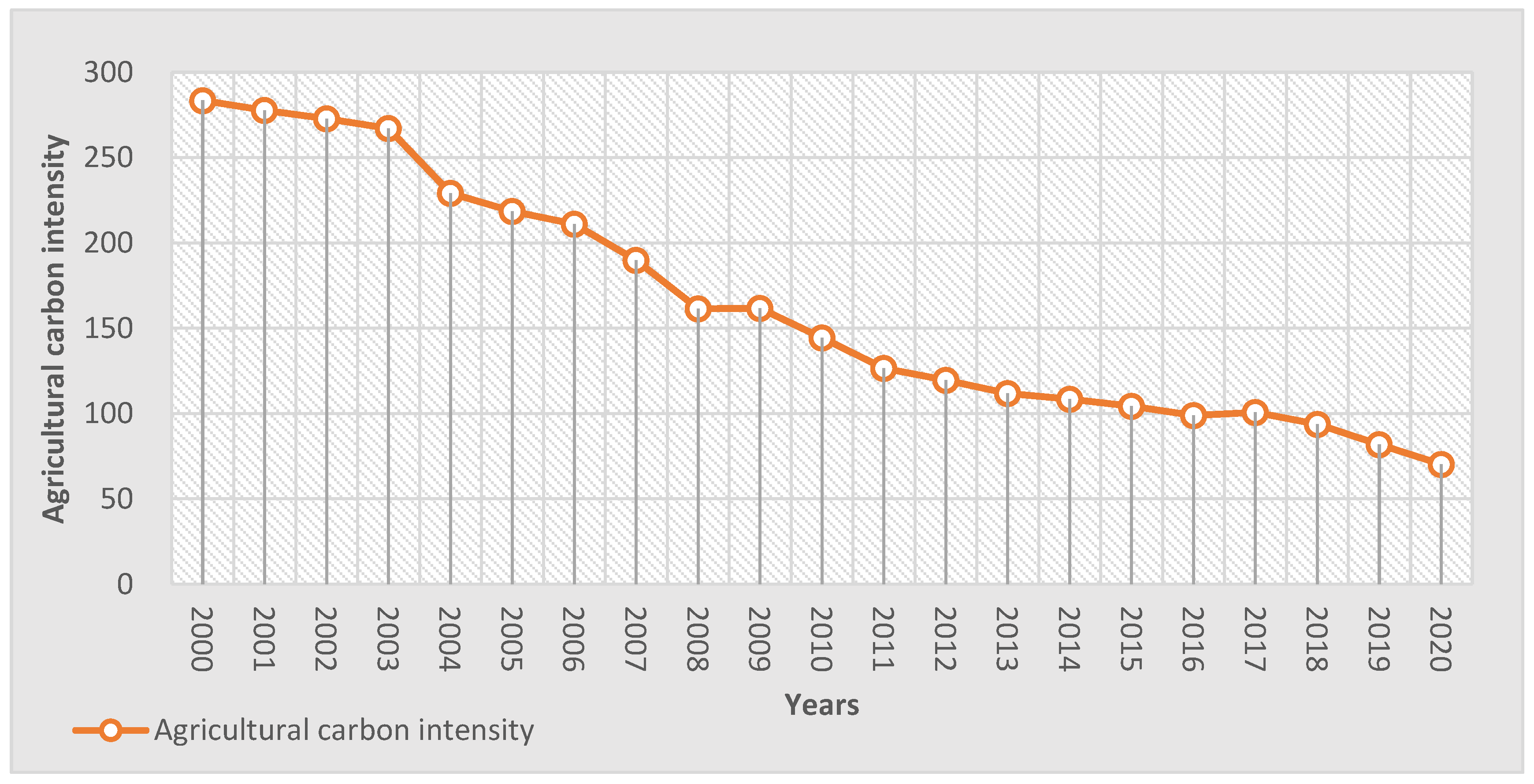
3.1. Analysis of the Current Situation of the Level of Financial Support to Agriculture and the Intensity of ACE

In this paper, the calculation method of agricultural CE intensity is expressed as [19]:
Agriculture   carbon   intensity = T o t a l   a g r i c u l t u r e   c a r b o n   e m i s s i o n s   A g r i c u l t u r e   o u t p u t   v a l u e + a n i m a l   b a n d r y   o u t p u t   v a l u e
Among them, the total amount of ACE is calculated by summing up the six aspects of ACE in Table 1: CE from agricultural diesel fuel consumed in the process of agricultural mechanization production; CE from chemical fertilizers that provide nutrients for plant growth; CE from pesticides used to regulate plant growth and control pest and disease disasters; CE from agricultural plastic films that play a role in moisturizing and heat preservation during planting; CE from fossil fuels consumed by electrical energy utilization during agricultural irrigation; and CE from ploughing land during crop sowing. The corresponding CE coefficients are shown in Table 1.
The specific calculation formula is:
E = E i = T i · ε i
Among them, E is the total amount of CE, E i is the CE amount produced by the i-th type of CE source, T i is the CE amount of the i-th type of CE source, and ε i is the CE coefficient of the i-th type of CE source.
During 2000–2020, the total amount of ACE shows a trend of first increasing and then decreasing, while the gross production value of agriculture and animal husbandry is basically in a state of growth. Moreover, its growth rate is higher than the growth rate of total ACE. Before 2015, the total amount of ACE was increasing, and the rate was relatively stable. However, after reaching 9.11 million tons in 2015, total ACE began to decline. The reason for this may be that the “Environmental Protection Law of the People’s Republic of China” was officially implemented on 1 January 2015, and the punishment for environmental pollution became heavier, effectively restraining the behavior of destroying the ecology in agricultural production. This series of data is based on publicly available data.
On the basis of the obtained data, the national agricultural CE intensity data from 2000 to 2020 are obtained by using the calculation formula above. It can be seen in Figure 1 that the intensity of ACE shows a clear downward trend. The ACE per 10,000 yuan of GDP has dropped from 0.28 tons in 2000 to 0.07 tons in 2020.
As shown in Figure 2, in 2000, the agricultural CE intensity of each province was relatively high. Among them, Shanxi, Shaanxi, and Ningxia produced more than 0.035 tons of ACE per 10,000 yuan of GDP, and the intensity of ACE significantly dropped from 2000 to 2010, and from 2010 to 2010. In 2020, the agricultural CE intensity of Jilin and Shanghai was above 0.01 ton/ten thousand yuan, which was relatively high. However, Sichuan, Guizhou, Tibet, and Ningxia had the lowest agricultural CE intensity, which was below 0.005 ton/10,000 tons, and the other provinces had the same CE intensity, which was between 0.005–0.01 ton/10,000 tons.
In addition, there were other factors affecting ACE. During this period (from 2000 to 2020) there were changes in product composition, watering methods, usage of fertilizer types, agroecological methods, changes in cultivated areas, changes in types of agricultural machines (for example, increases in machines using less fuel), etc. During the development of agricultural activities, the use of fertilizers with different compositions will directly affect the carbon emissions generated in agricultural production activities, and the use of environmentally friendly fertilizers will effectively reduce carbon emissions. Similarly, the replacement of production tools can effectively promote carbon emissions in agricultural activities. As mentioned earlier, the introduction of machines with low fuel consumption or the replacement of regressive and pollution-prone machines with green and environmentally friendly new energy machines will effectively reduce the carbon emissions of this production activity. This is exactly what financial support should pay attention to.

3.2. Research Model

3.2.1. Explained Variable

In this paper, the CE intensity (Carbon) is selected as the explained variable, and the expression method is: the ratio of the total agricultural CE to the total agricultural and animal husbandry production value [20].

3.2.2. Core Explanatory Variable

The level of financial support to agriculture is the core explanatory variable of this paper. It is measured by the ratio of fiscal expenditure to support agriculture to total fiscal expenditure. This indicator can show the importance of fiscal expenditure on agriculture.

3.2.3. Control Variable

This paper selects the level of urbanization and the degree of agricultural disasters. It is noted that the natural disasters mentioned here refer to the natural phenomena that bring harm to human existence or damage to the human living environment, including droughts, high temperatures, low temperatures, cold waves, floods, typhoons, tornadoes, flame tornadoes, hail, frost, rainstorms, blizzards, freezing rain, acid rain, fog, winds, icing, haze, earthquakes, tsunamis, landslides, debris flow, dust, sand, dust storms, lightning, thunderstorms, ball lightning, volcanic eruption, etc. The agricultural industry structure, the degree of agricultural mechanization, the education level of farmers, the scale of agricultural planting, and the level of economic development are used as control variables.
  • Urbanization level (Urban) is expressed as the ratio of urban population to total population. Urbanization has a certain influence on ACE, but the direction of influence may vary in different regions. Urbanization will change the scale of agricultural land and the scale of rural labor, resulting in changes in agricultural production factors, which in turn will affect ACE.
  • The degree of agricultural disaster (Disaster) is expressed as the ratio of the affected area of crops to the total sown area. The degree of disaster in agriculture will affect the output value. If the degree of disaster in a certain area is high, it will lead to a reduction in production in the current year, and farmers may change the amount of factor inputs in the later period, thereby affecting CE.
  • Agricultural industrial structure (Structure) is expressed by the ratio of the total agricultural output value to the total output value of agriculture, forestry, animal husbandry, and by-fishing. Because agriculture, forestry, animal husbandry, and fishing have different industrial characteristics, the CE produced are different.
  • The degree of agricultural mechanization (Machine) is expressed by the ratio of agricultural machinery power to the rural population. Machinery already plays an important role in agricultural production and, generally speaking, the more machinery is used, the higher the CE.
  • The education level of farmers (Education) is expressed by the average years of education of the rural population. With different education levels, farmers have different degrees of acceptance of the concept of green production. The education level of the labor force in rural households is mainly divided into five levels: illiterate or very little literate, primary school, junior high school, high school, college or above. Considering the actual situation, the number of years of education for those with little or no literacy is represented by the median value of 3 in the primary school system, and the others are represented by 6, 9, 12, and 16, respectively. Pi represents the number of people at different levels of education, and the formula for calculating the average years of education is [21]:
(P1 × 3 + P2 × 6 + P3 × 9 + P4 × 12 + P5 × 16)/(P1 + P2 + P3 + P4 + P5)
6.
The scale of agricultural planting (Plant) is expressed by the ratio of the sown area of crops to the rural population. That is, the sown area per capita.
7.
The level of economic development (Economics) is expressed by the ratio of the total production value of agriculture, forestry, animal husbandry, and by-fishing to the rural population. It is generally believed that, in areas with a high level of economic development, the market for agricultural production factors and agricultural products is more mature.
Considering the availability of data, this paper takes 31 provinces (including municipalities and autonomous regions) in mainland China as the research object, and does not include Hong Kong, Macao, and Taiwan into the scope of this research. The time span is 2000–2020, and a total of 651 samples are used for the observations made in this paper. The data are all from the National Bureau of Statistics, China Statistical Yearbook, China Price Statistical Yearbook, and China Rural Statistical Yearbook. In order to eliminate the influence of the dimension on the results, the variables have been standardized before being substituted into the model. After standardization, the observed values of each variable are between [0, 1]. The processing formula is:
X′ = (XXmin)/(XmaxXmin)
Table 2 shows the descriptive statistics of each variable.

4. Results

This paper uses Geoda software to calculate the Moran’s I index of China’s ACE from 2000 to 2020. The calculation results are shown in Table 3:
The value range of I is between [−1, 1]. When I < 0, it indicates that there is a negative spatial correlation. When I = 0, it indicates that there is no spatial correlation. When I > 0, it indicates that there is a positive spatial correlation. It can be seen that, except for a few years, the Moran’s I index of agricultural CE intensity in other years is significantly positively correlated at the level of 5%, and the spatial correlation degree in recent years has become more significant.
From the Morans’ I index analyzed above, we can see that the intensity of ACE exhibits spatial autocorrelation, which requires the use of a spatial econometric model. In this paper, the multicollinearity diagnosis of the panel data is carried out, and the results show that the VIF values are all less than 10, indicating that there is no serious multicollinearity among the variables (Table 4).
In this paper, Geoda software is used to form a queen-based contiguity weight matrix in the map. If two provinces have a common edge or point, their distance is set to 1, and if there is no common edge or point between two provinces, their distance is set to 0. Since Hainan is an “isolated island” city, when constructing the spatial weight matrix, Hainan and Guangdong are set as adjacent provinces. The constructed spatial weight matrix w is imported into Stata and normalized.
There are three main spatial econometric models: the spatial error model, the spatial lag model, and the spatial Durbin model. In order to test which model is more suitable, this paper conducts the Lagrange multiplier LM test on the panel data.
It can be seen from Table 5 that the spatial error and spatial lag of LM are significant, so the null hypothesis should be rejected and the spatial Durbin model should be used. Then, the LR test and the Wald test are used to further verify whether the spatial Durbin model would degenerate into a spatial error model or a spatial lag model (Table 6).
Both the LR test and the Wald test show that the spatial Durbin model neither degenerates into a spatial lag model nor into a spatial error model, while the Hausman test results show that a random effect model should be used instead of a fixed effect model. Based on the above analysis, it is finally determined that the model in this paper is the spatial Doberman model of random effects. The formula is as follows:
Yit = ρWijYjt + βXit + γWijXjt + εij
Among them, Yit represents the dependent variable of i province in year t; X is an nxk matrix (n is the number of provinces, k is the number of exogenous independent variables); Wij is the nxn order spatial distance 0–1 matrix (if the i and j provinces are adjacent, the W value is 1; if the i and j provinces are not adjacent, the W value is 0); WX and WY are the spatial lag terms of the independent variable and dependent variable, respectively, and ρ, β, and γ are the parameters to be estimated.
The effects of the spatial Durbin model are decomposed into direct effects and indirect effects. The direct effect refers to the degree of influence of the independent variable of the province on the dependent variable of the province, and the indirect effect refers to the degree of influence of the independent variable of the province on the dependent variable of the neighboring province. The results are shown in Table 7:

5. Analysis and Discussion

Compared with the research results of other scholars, from the empirical analysis results of this paper, it can be seen that every 1% increase in the level of financial support to agriculture will cause a 0.2071% increase in CE intensity. Among them, 0.1357% are caused by direct effects, and 0.0714% are caused by indirect effects, and both pass the significance level test. It shows that the increase in the level of the support in a province will not only increase the CE intensity of the province, but also increase the CE intensity of its neighboring provinces, and will have a greater direct effect on the province. In the early agricultural modernization process, a large number of labors are transferred to the agricultural production sector, and the financial investment in agriculture was also increased, but it caused serious environmental pollution. At this stage, when the level of financial expenditure is higher, farmers will increase their expectations of agricultural output value, the use of machinery, chemical fertilizers, etc., and blindly expand production, which will lead to an increase in the intensity of ACE in this province and neighboring provinces.
In addition, factors such as the urbanization rate, the degree of agricultural mechanization, the education level of farmers, and the agricultural planting scale all have significant spatial effects, while the overall spatial effect of agricultural disaster severity, agricultural industrial structure, and economic development level is not significant.
The following conclusions can be drawn by summarizing the model data:
8.
The agricultural CE intensity has spatial autocorrelation. The global Moran’s I index of agricultural CE intensity from 2000 to 2020 is calculated by Geoda software to be positive. Except for 2008 and 2011, all other years pass the significance test, and the spatial correlation degree of agricultural CE intensity is more obvious in recent years.
9.
According to the measurement results of the spatial Durbin model, the degree of agricultural mechanization positively affects the agricultural CE intensity of the province, and negatively affects the agricultural CE intensity of neighboring provinces. The agricultural industrial structure and economic development level negatively affect the agricultural CE intensity of this province, and positively affect the agricultural CE intensity of neighboring provinces. The level of fiscal expenditure, the degree of agricultural disasters, and the scale of agricultural planting all have a positive influence on the agricultural CE intensity of this province and neighboring provinces. The urbanization rate and the education level of farmers have a negative influence on the agricultural CE intensity of this province and neighboring provinces.
10.
From the decomposition effect of the spatial Durbin model, it can be seen that the level of fiscal expenditure has a much greater influence on the ACE of this province than it has on neighboring provinces. When the level of fiscal expenditure increases by 1%, the CE intensity of agriculture will increase by 0.2071%.
According to the above analysis of the mechanism of financial support to agriculture on ACE, the level of the support increased CE intensity. It may be because the government’s financial investment pursues short-term economic benefits or political performance, or it may be because the investment structure is unreasonable and the technical support is insufficient.
Based on the above conclusions, the following recommendations are given:
11.
It is necessary to optimize the structure of financial support to agriculture. Through the above analysis, the increase in the level of the support does not reduce the intensity of ACE, but it does significantly increase the intensity of ACE. This shows that the high-input and extensive agricultural production methods cannot improve the ecological benefits, even if financial support is increased. With the increase in financial investment, its use must be rationally planned, the proportion of investment in agricultural infrastructure construction and scientific and technological research and development must be increased, and the ecological orientation of financial expenditure in support of agriculture must be enhanced, which makes the best use of financial funds and can reduce ACE, while promoting the improvement of agricultural economic benefits.
12.
It is necessary to implement reasonable subsidies for agricultural production. The government needs to improve relevant policies, use financial subsidies to support agriculture for farmers who conduct low-carbon production, or subsidize organic fertilizers to reduce the cost for farmers applying organic fertilizers, and positively encourage farmers to adjust production methods and rationally use agricultural production factors.
13.
Provinces need to collaborate to promote agricultural emission reduction. The intensity of ACE has obvious spatial effects. Therefore, it is necessary to pay attention to the coordinated development between adjacent provinces, optimize the spatial and regional distribution structure of agricultural finance, and achieve win-win cooperation. Moreover, the provinces need to exchange and learn from each other advanced agricultural production technologies, and jointly use production methods such as water-saving and fertilizer-saving to improve the utilization rate of production factors. In addition, it is necessary to introduce a CE trading mechanism in agriculture to give importance to the role of the market in reducing CE.

6. Conclusions

Based on the panel data of 31 provinces (including municipalities and autonomous regions) from 2000 to 2020, this paper used Geoda software to construct a spatial distance weight matrix, and established a random effect spatial Durbin model to analyze the influence of the level of support on the intensity of ACE, and reached the following conclusions: (1) The agricultural CE intensity has spatial autocorrelation. (2) The degree of agricultural mechanization, agricultural industrial structure, economic development level, financial expenditure level, agricultural disaster degree, agricultural planting scale, urbanization rate, and education level of farmers are all factors that affect the intensity of ACE. (3) The influence of fiscal expenditure on ACE in this province is much greater than that on neighboring provinces. Based on the above conclusions, the following recommendations were made: (1) It is necessary to optimize the structure of fiscal support for agriculture. (2) Provinces should cooperate to promote agricultural emission reduction. The follow-up research work of this paper will introduce more influencing factors of ACE for analysis, and intelligently process the model to achieve real-time dynamic analysis of the influencing factors of ACE.

Author Contributions

Methodology, Y.G.; Software, M.C. and X.H.; Resources, Y.G.; Writing—original draft, M.C.; Writing—review & editing, X.H.; Supervision, Y.G. All authors have read and agreed to the published version of the manuscript.

Funding

This study was supported by the Economics School of Anhui University Sciences Research Project (Z010111018).

Institutional Review Board Statement

Not applicable.

Informed Consent Statement

Not applicable.

Data Availability Statement

The data that support the findings of this study are available from the corresponding author upon request.

Conflicts of Interest

The authors declare that they have no conflicts of interest regarding the publication of this paper.

References

  1. Xia, S.; You, D.; Tang, Z.; Yang, B. Analysis of the spatial effect of fiscal decentralization and environmental decentralization on carbon emissions under the pressure of officials’ promotion. Energies 2021, 14, 1878. [Google Scholar] [CrossRef]
  2. Yang, Y.; Yang, X.; Tang, D. Environmental regulations, Chinese-style fiscal decentralization, and carbon emissions: From the perspective of moderating effect. Stoch. Environ. Res. Risk Assess. 2021, 35, 1985–1998. [Google Scholar] [CrossRef]
  3. Yin, Y.; Xi, F.M.; Bing, L.F.; Wang, J.Y.; Li, J.Y.; LY, D.; Liu, L. Accounting and red uction path of carbon emission firom facility agriculture in China. Ying Yong Sheng Tai Xue Bao (J. Appl. Ecol.) 2021, 32, 3856–3864. [Google Scholar]
  4. Mor, S.; Madan, S.; Prasad, K.D. Artificial intelligence and carbon footprints: Roadmap for Indian agriculture. Strateg. Change 2021, 30, 269–280. [Google Scholar] [CrossRef]
  5. Borychowski, M.; Grzelak, A.; Popławski, Ł. What drives low-carbon agriculture? The experience of farms from the Wielkopolska region in Poland. Environ. Sci. Pollut. Res. 2022, 29, 18641–18652. [Google Scholar] [CrossRef]
  6. Wang, R.; Feng, Y. Research on China’s agricultural carbon emission efficiency evaluation and regional differentiation based on DEA and Theil models. Int. J. Environ. Sci. Technol. 2021, 18, 1453–1464. [Google Scholar] [CrossRef]
  7. Koondhar, M.A.; Shahbaz, M.; Ozturk, I.; Randhawa, A.A.; Kong, R. Revisiting the relationship between carbon emission, renewable energy consumption, forestry, and agricultural financial development for China. Environ. Sci. Pollut. Res. 2021, 28, 45459–45473. [Google Scholar] [CrossRef]
  8. Gokmenoglu, K.K.; Taspinar, N. Testing the agriculture-induced EKC hypothesis: The case of Pakistan. Environ. Sci. Pollut. Res. 2018, 25, 22829–22841. [Google Scholar] [CrossRef]
  9. Han, H.; Zhong, Z.; Guo, Y.; Xi, F.; Liu, S. Coupling and decoupling effects of agricultural carbon emissions in China and their driving factors. Environ. Sci. Pollut. Res. 2018, 25, 25280–25293. [Google Scholar] [CrossRef]
  10. Vandyck, T.; Keramidas, K.; Kitous, A.; Spadaro, J.V.; Van Dingenen, R.; Holland, M.; Saveyn, B. Air quality co-benefits for human health and agriculture counterbalance costs to meet Paris Agreement pledges. Nat. Commun. 2018, 9, 1–11. [Google Scholar] [CrossRef]
  11. Rehman, A.; Ma, H.; Ahmad, M.; Ozturk, I.; Chishti, M.Z. How do climatic change, cereal crops and livestock production interact with carbon emissions? Updated evidence from China. Environ. Sci. Pollut. Res. 2021, 28, 30702–30713. [Google Scholar] [CrossRef]
  12. Li, P.; Xiao, C.; Feng, Z. Swidden agriculture in transition and its roles in tropical forest loss and industrial plantation expansion. Land Degrad. Dev. 2022, 33, 388–392. [Google Scholar] [CrossRef]
  13. Gokmenoglu, K.K.; Taspinar, N.; Kaakeh, M. Agriculture-induced environmental Kuznets curve: The case of China. Environ. Sci. Pollut. Res. 2019, 26, 37137–37151. [Google Scholar] [CrossRef]
  14. Niles, M.T.; Ahuja, R.; Barker, T.; Esquivel, J.; Gutterman, S.; Heller, M.C.; Mango, N.; Portner, D.; Raimond, R.; Tirado, C.; et al. Climate change mitigation beyond agriculture: A review of food system opportunities and implications. Renew. Agric. Food Syst. 2018, 33, 297–308. [Google Scholar] [CrossRef]
  15. Fang, K.; Li, S.; Ye, R.; Zhang, Q.; Long, Y. New progress in global climate governance: A review on the allocation of regional carbon emission allowance. Shengtai Xuebao/Acta Ecol. Sin. 2020, 40, 10–23. [Google Scholar]
  16. Balsalobre-Lorente, D.; Driha, O.M.; Bekun, F.V.; Osundina, O.A. Do agricultural activities induce carbon emissions? The BRICS experience. Environ. Sci. Pollut. Res. 2019, 26, 25218–25234. [Google Scholar] [CrossRef]
  17. Kumar, A.; Singh, V.; Shabnam, S.; Oraon, P.R. Carbon emission, sequestration, credit and economics of wheat under poplar based agroforestry system. Carbon Manag. 2020, 11, 673–679. [Google Scholar] [CrossRef]
  18. Usman, A.; Quan-Lin, L.; Abdullah, A.M.; Shakib, M.; Wasim, I. Nexus between agro-ecological efficiency and carbon emission transfer: Evidence from China. Environ. Sci. Pollut. Res. Int. 2021, 28, 18995–19007. [Google Scholar]
  19. Aziz, N.; Sharif, A.; Raza, A.; Rong, K. Revisiting the role of forestry, agriculture, and renewable energy in testing environment Kuznets curve in Pakistan: Evidence from Quantile ARDL approach. Environ. Sci. Pollut. Res. 2020, 27, 10115–10128. [Google Scholar] [CrossRef]
  20. Singh, S.P.; Naresh, R.K.; Kumar, S.; Kumar, V.; Mahajan, N.C.; Mrunalini, K.; Chandra, M.S.; Prasad, K.K. Conservation agriculture effects on aggregates carbon storage potential and soil microbial community dynamics in the face of climate change under semi-arid conditions: A review. J. Pharmacogn. Phytochem. 2019, 8, 59–69. [Google Scholar]
  21. Guerrero, S.; Nakagawa, M. Productivity improvements and reducing GHG emission intensity in agriculture go together–up to a point. EuroChoices 2019, 18, 24–25. [Google Scholar] [CrossRef]
Figure 1. National agricultural CE intensity from 2000 to 2020. Data sources: China Rural Statistical Yearbook (2001–2021), China Price Statistical Yearbook (2021).
Sustainability 15 02228 g001
Figure 2. Agricultural CE intensity of each province in 2000, 2010, and 2020. Data sources: China Rural Statistical Yearbook (2001–2021), China Price Statistical Yearbook (2021).
Sustainability 15 02228 g002
Table 1. The main CE sources of agriculture (planting industry) and their CE coefficients.
CE SourceCE Factor
Diesel fuel0.5927 kg/kg
Fertilizer0.8956 kg/kg
Pesticide4.9341 kg/kg
Agricultural film5.18 kg/kg
Irrigation20.476 kg/hm2
Sowing312.6 kg/km2
Table 2. Descriptive statistics of each variable.
VariableVariable DescriptionSample SizeAverage ValueMedianStandard DeviationMinimumMaximum Value
CarbonAgricultural CE intensity (t/10,000 yuan-1)6510.01600.01400.008000.003000.0500
FinanceThe level of financial support to agriculture6510.09600.09700.03900.009000.204
UrbanUrbanization rate6510.5090.5000.1570.1890.896
DisasterDegree of agricultural disaster6510.2260.1970.15900.936
StructureAgricultural industry structure6510.5230.5100.08700.3020.746
MachineAgricultural mechanization degree (kw/person)6511.3481.1820.7910.2266.213
EducationThe education level of farmers6517.6247.7250.7534.7429.912
PlantAgricultural planting scale (ha/person)6510.2530.2120.1550.03101.367
EconomicsEconomic development level (10,000 yuan/person)6511.2131.0200.8580.1454.531
Table 3. Moran’s I index of agricultural CE intensity from 2000 to 2020.
YearsIzp-ValueYearsIzp-Value
20000.1591.7990.03620110.0620.8790.19
20010.1381.5990.05520120.171.8810.03
20020.1511.7110.04320130.1261.4690.071
20030.2652.7630.00320140.1271.4820.069
20040.1431.6260.05220150.1541.7270.042
20050.1090.7580.02420160.2092.2190.013
20060.1571.7520.0420170.1791.9610.025
20070.1511.7060.04420180.2362.480.007
20080.091.1360.12820190.2983.0380.001
20090.1121.3460.08920200.3333.3660
20100.1071.2940.098
Table 4. Multicollinearity diagnosis.
VariableVIF1/VIF
Urban3.1100.321
Economics3.0600.327
Education2.5400.393
Machine2.4000.416
Plant2.4000.417
Finance1.9100.525
Structure1.4100.710
Disaster1.3600.733
Mean2.2740.480
Table 5. LM test results.
TestStatistical Valuep-Value
Spatial error model
(Spatial error)
Moran’s I20.9920.00
Lagrange multiplier414.1260.00
Robust Lagrange multiplier269.3070.00
Spatial lag model
(Spatial lag)
Lagrange multiplier160.5680.00
Robust Lagrange multiplier15.7500.00
Table 6. LR test and Wald test results.
TestTest PurposeTest Result
LRWhether SDM will degrade to SARLR chi2(8) = 53.95Prob > chi2 = 0.000
Whether SDM will degrade to SEMLR chi2(8) = 46.72Prob > chi2 = 0.000
WaldWhether SDM will degrade to SARchi2(8) = 47.33Prob > chi2 = 0.000
Whether SDM will degrade to SEMchi2(8) = 69.18Prob > chi2 = 0.000
Table 7. Effect decomposition of the spatial Durbin model.
VariableLR_DirectLR_IndirectLR_Total
Finance0.1357 ***0.0714 ***0.2071 ***
(0.0313)(0.0209)(0.0495)
Urban−0.2166 ***−0.3542 ***−0.5708 ***
(0.0436)(0.1156)(0.1265)
Disaster0.01460.00780.0224
(0.0182)(0.0098)(0.0279)
Structure−0.03190.1280 **0.0962
(0.0298)(0.0621)(0.0657)
Machine0.2157 ***−0.9289 ***−0.7132 ***
(0.0595)(0.1222)(0.1363)
Education−0.1659 ***−0.5808 ***−0.7467 ***
(0.0603)(0.1128)(0.1233)
Plant0.1960 **0.1027 **0.2987 **
(0.0939)(0.0523)(0.1437)
Economics−0.2532 ***0.2112 **−0.0420
(0.0320)(0.0833)(0.0897)
N651R20.303
Note: Robust t-statistics in parentheses *** p < 0.01, ** p < 0.05.
Disclaimer/Publisher’s Note: The statements, opinions and data contained in all publications are solely those of the individual author(s) and contributor(s) and not of MDPI and/or the editor(s). MDPI and/or the editor(s) disclaim responsibility for any injury to people or property resulting from any ideas, methods, instructions or products referred to in the content.

