


Predicting Traffic Casualties Using Support Vector Machines with Heuristic Algorithms: A Study Based on Collision Data of Urban Roads

Abstract
:1. Introduction
1.1. Literature Review
1.2. Related Work
2. Data
3. Methodology
3.1. Support Vector Machine
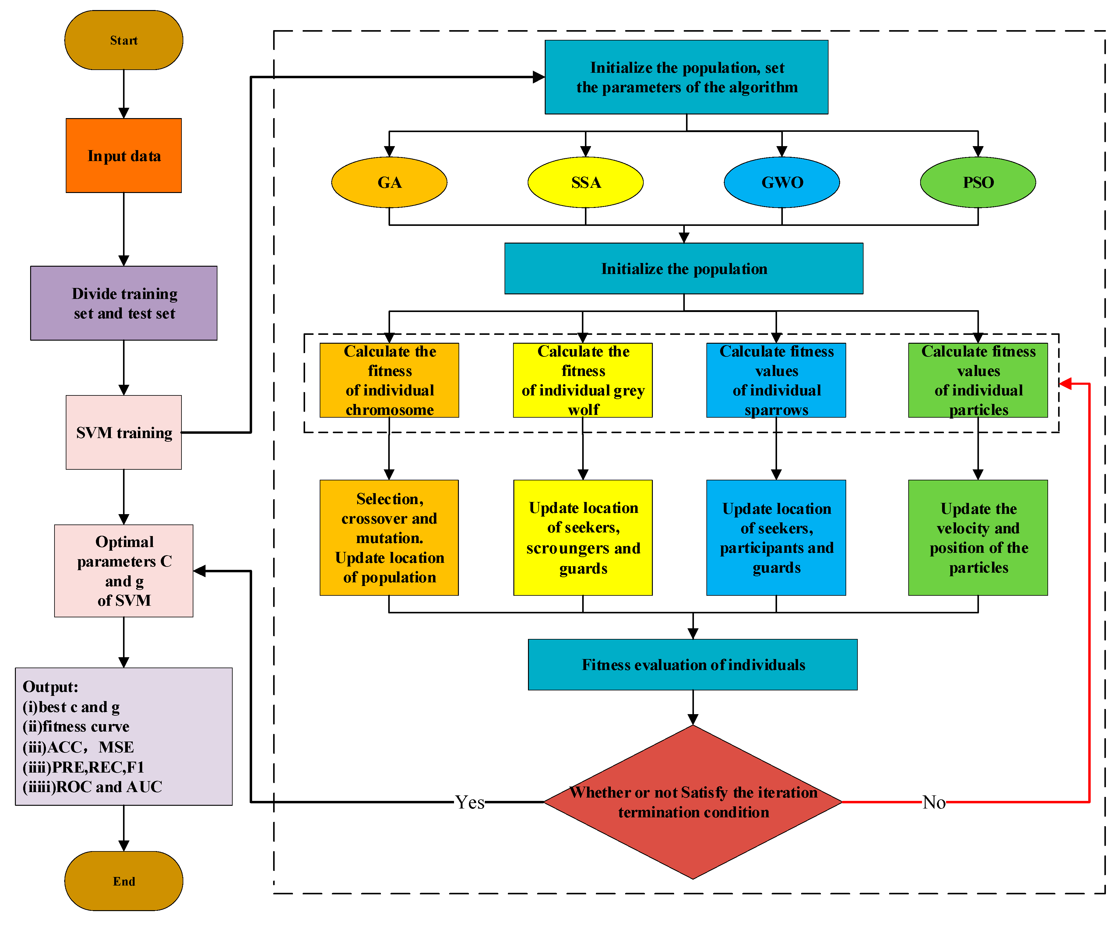
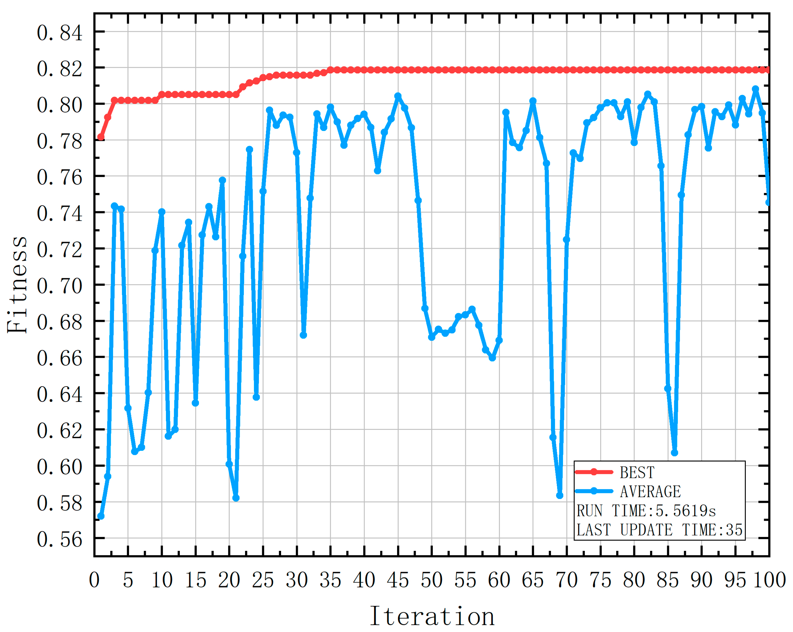
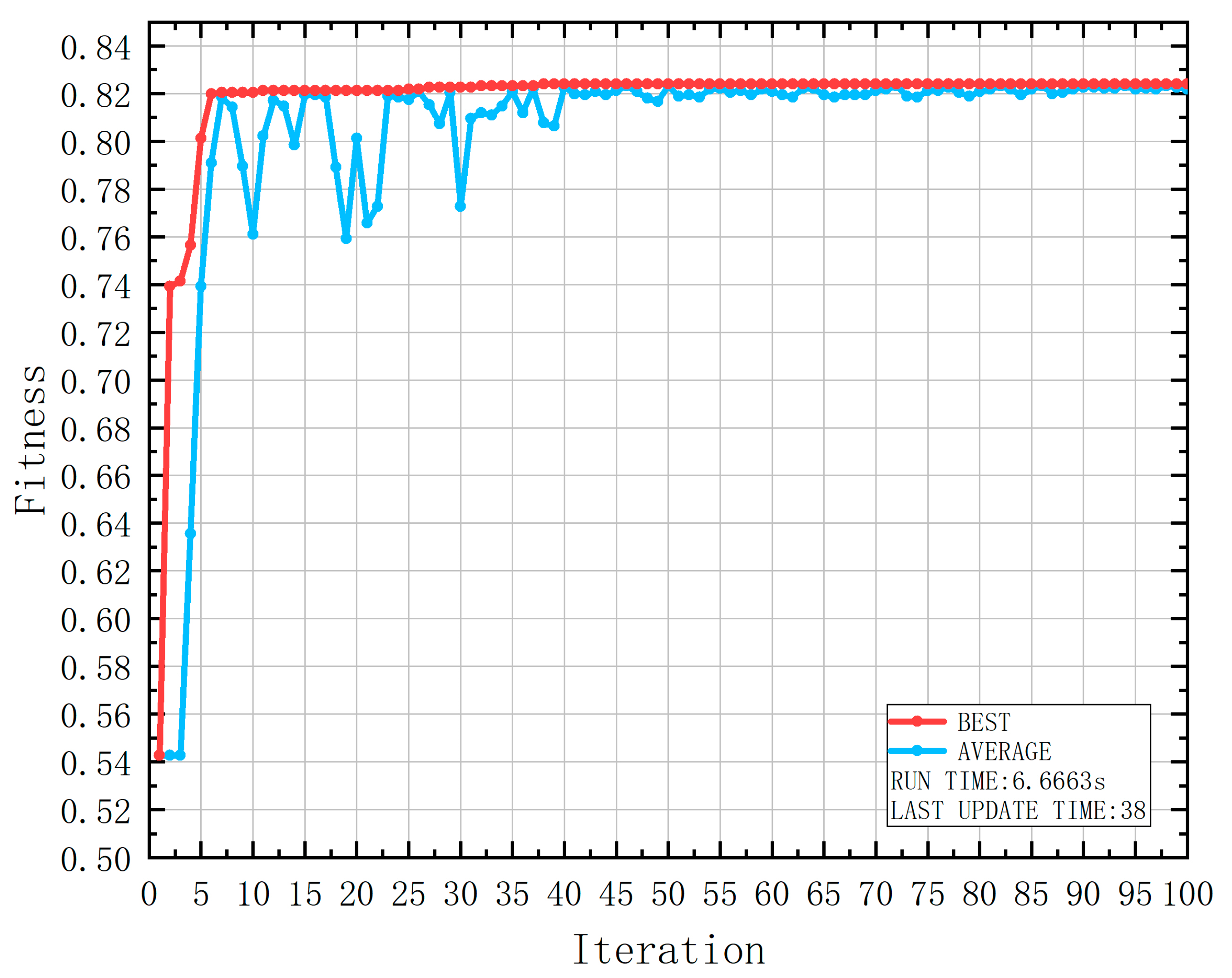
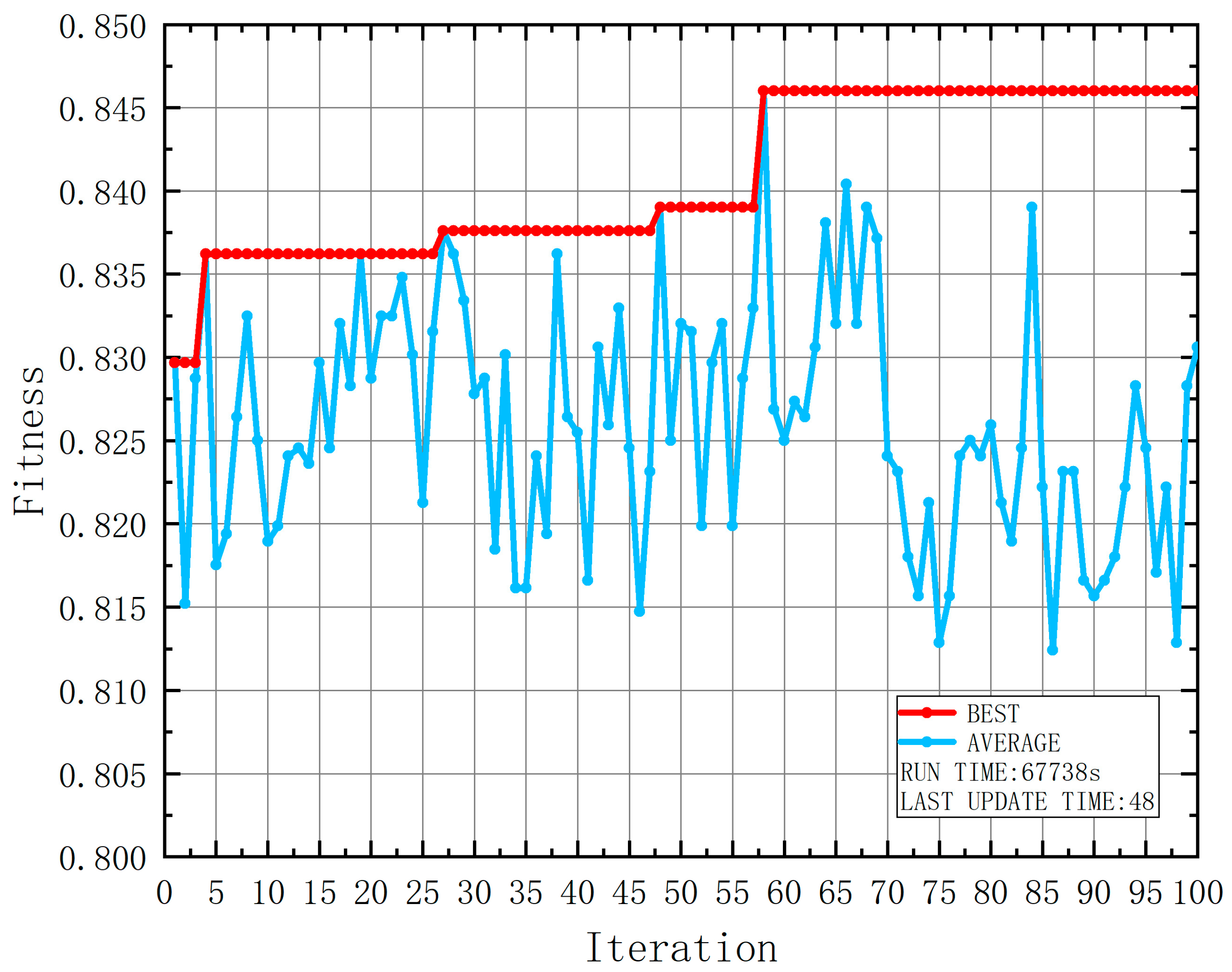
3.2. SVM Optimized by Multiple Heuristic Algorithms
- (i)
- GA

| Maximum evolutionary quantity | 100 |
| Maximum population size | 20 |
| Crossover probability | 0.4 |
| Mutation probability | 0.01 |
- (ii)
- SSA
| Warning value of sparrow | 0.8 |
| Search dimension | 2 |
| Maximum population size | 20 |
| Maximum evolutionary quantity | 100 |
- (iii)
- GWO
| Value seeking range of wolf | 2 |
| Maximum evolutionary quantity | 100 |
| Warning value of sparrow | 20 |
- (iv)
- PSO
| Search dimension | 2 |
| Local search ability | 1.5 |
| Global search ability | 1.7 |
| Maximum evolutionary quantity | 100 |
| Maximum population size | 20 |
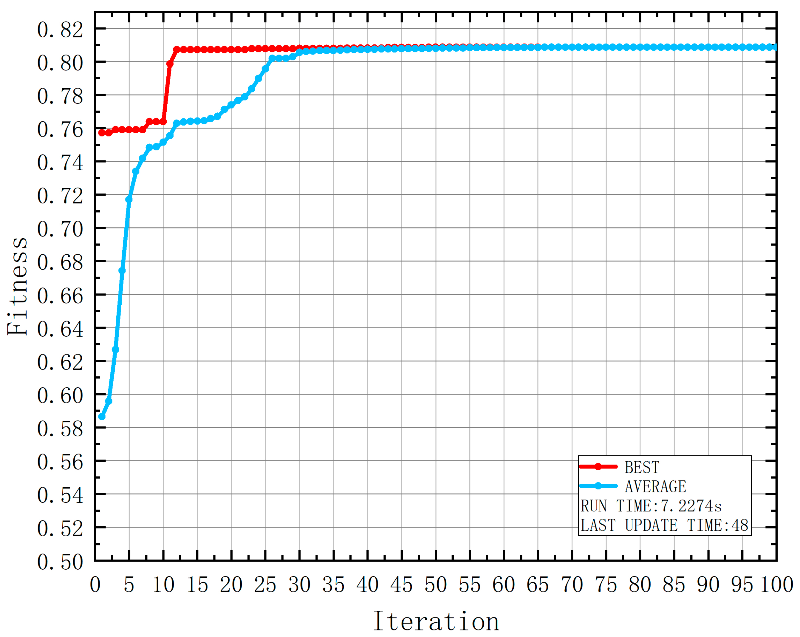
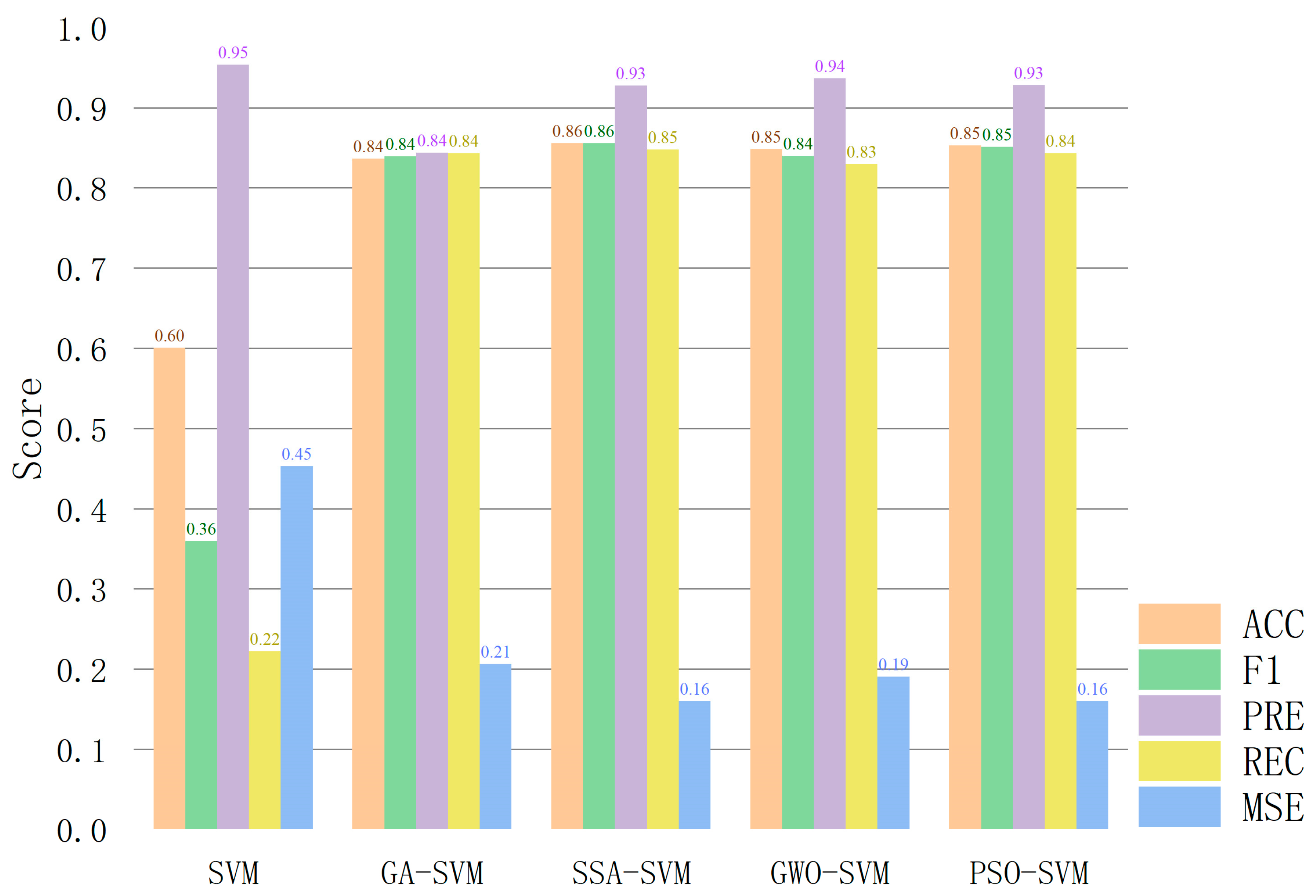
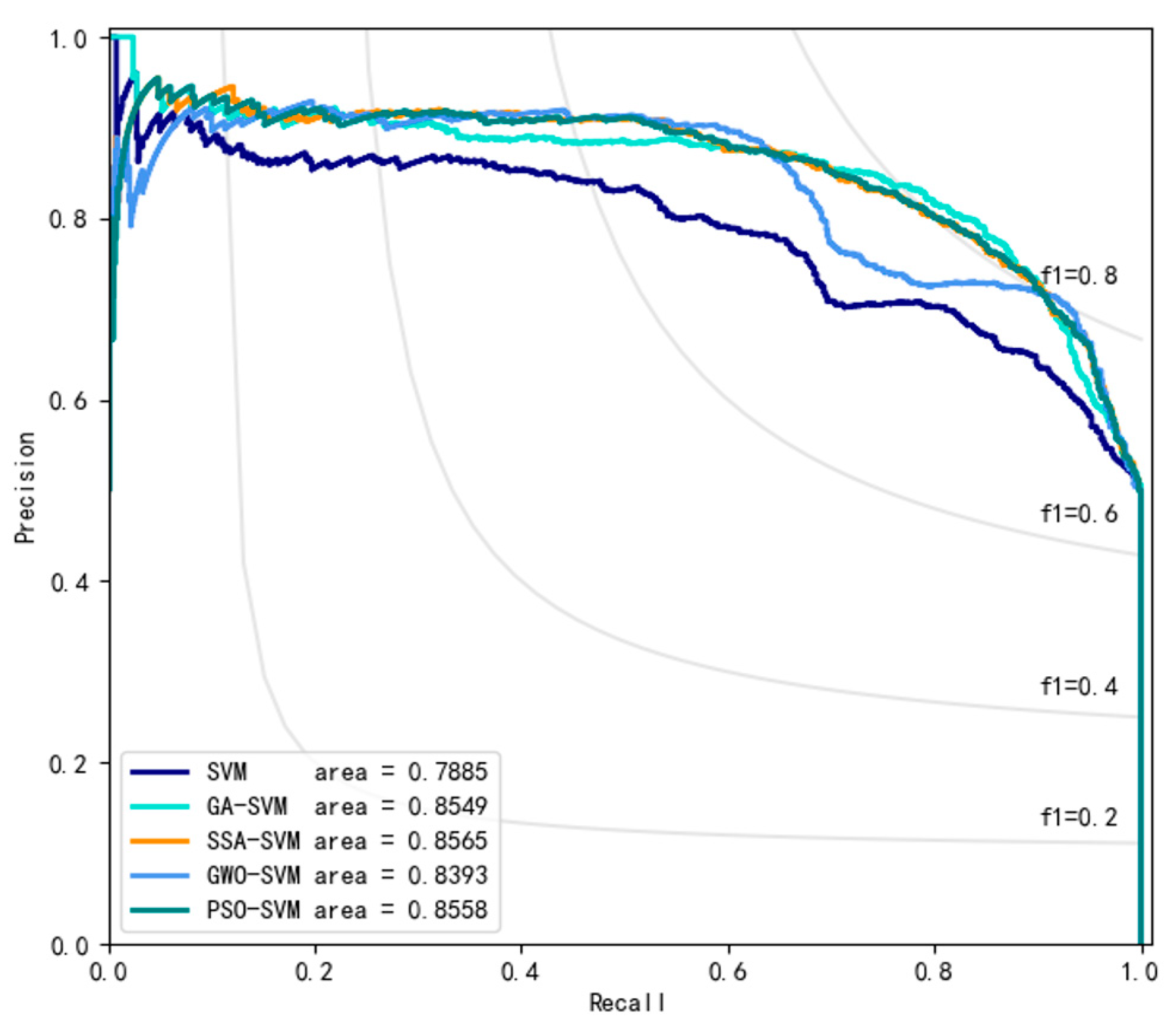
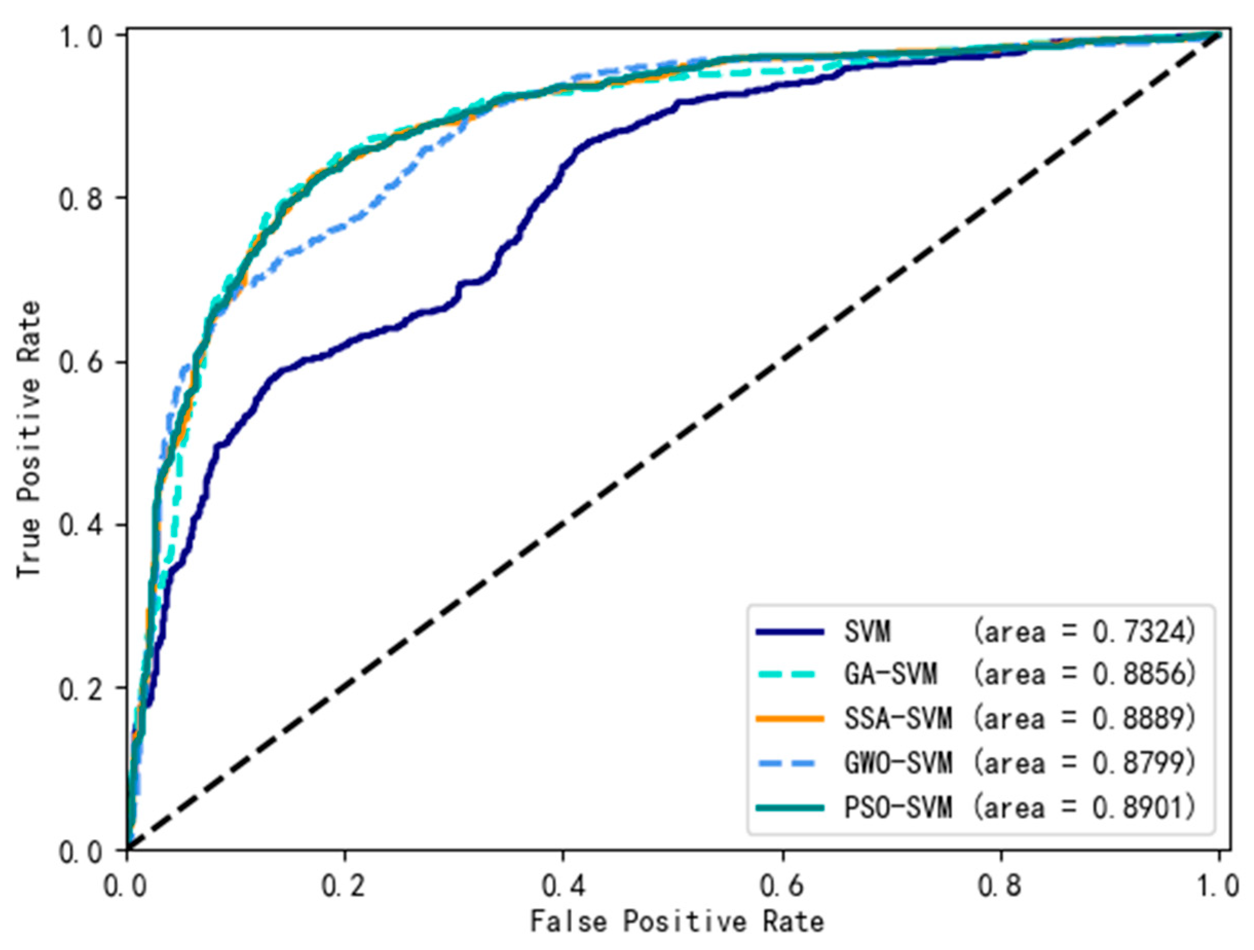
4. Experimental Result
5. Conclusions
Author Contributions
Funding
Institutional Review Board Statement
Informed Consent Statement
Data Availability Statement
Conflicts of Interest
References
- Li, Z.Y.; Hao, T.X.; Zheng, R. The Relationship between Transportation Industry Efficiency, Transportation Structure, and Regional Sustainability Development in China: Based on DEA and PVAR Models. Sustainability 2022, 14, 10267. [Google Scholar] [CrossRef]
- Zhang, L.Y.; Zhang, M.; Tang, J.Z.; Ma, J.; Duan, X.K.; Sun, J.; Hu, X.F.; Xu, S.C. Analysis of Traffic Accident Based on Knowledge Graph. J. Adv. Transp. 2022, 2022, 3915467. [Google Scholar] [CrossRef]
- Jackisch, J.; Sethi, D.; Mitis, F.; Szymanski, T.; Arra, I. European Facts and the Global Status Report on Road Safety 2015. Inj. Prev. 2016, 22, A29. [Google Scholar] [CrossRef]
- Zheng, M.; Li, T.; Zhu, R.; Chen, J.; Ma, Z.F.; Tang, M.J.; Cui, Z.Q.; Wang, Z. Traffic Accident’s Severity Prediction: A Deep-Learning Approach-Based CNN Network. IEEE Access 2019, 7, 39897–39910. [Google Scholar] [CrossRef]
- Sabet, F.P.; Tabrizi, K.N.; Khankeh, H.R.; Saadat, S.; Abedi, H.A.; Bastami, A. Road Traffic Accident Victims’ Experiences of Return to Normal Life: A Qualitative Study. Iran. Red Crescent Med. J. 2016, 18, 7. [Google Scholar]
- Handayani, A.S.; Putri, H.M.; Soim, S.; Husni, N.L.; Rusmiasih; Sitompul, C.R. Intelligent Transportation System For Traffic Accident Monitoring. In Proceedings of the 3rd International Conference on Electrical Engineering and Computer Science (ICECOS), Batam, Indonesia, 2–3 October 2019; IEEE: Batam, Indonesia, 2019; pp. 156–161. [Google Scholar]
- Wongcharoen, S.; Senivongse, T. Twitter Analysis of Road Traffic Congestion Severity Estimation. In Proceedings of the 13th International Joint Conference on Computer Science and Software Engineering (JCSSE), Khon Kaen, Thailand, 13–15 July 2016; IEEE: Khon Kaen, Thailand, 2016; pp. 76–81. [Google Scholar]
- Zhang, J.H. Integration Theory and Optimal Application of the Traffic Accident Management System. In Proceedings of the International Conference on Cyber Security Intelligence and Analytics (CSIA), Shenyang, China, 21–22 February 2019; Springer International Publishing Ag: Shenyang, China, 2019; pp. 99–104. [Google Scholar]
- Kockelman, K.M.; Kweon, Y.-J. Driver injury severity: An application of ordered probit models. Accid. Anal. Prev. 2002, 34, 313–321. [Google Scholar] [CrossRef] [PubMed]
- Kaplan, S.; Prato, C.G. Risk factors associated with bus accident severity in the United States: A generalized ordered logit model. J. Saf. Res. 2012, 43, 171–180. [Google Scholar] [CrossRef]
- Eluru, N.; Bhat, C.R.; Hensher, D.A. A mixed generalized ordered response model for examining pedestrian and bicyclist injury severity level in traffic crashes. Accid. Anal. Prev. 2008, 40, 1033–1054. [Google Scholar] [CrossRef]
- Al-Ghamdi, A.S. Using logistic regression to estimate the influence of accident factors on accident severity. Accid. Anal. Prev. 2002, 34, 729–741. [Google Scholar] [CrossRef]
- Kononen, D.W.; Flannagan, C.A.C.; Wang, S.C. Identification and validation of a logistic regression model for predicting serious injuries associated with motor vehicle crashes. Accid. Anal. Prev. 2011, 43, 112–122. [Google Scholar] [CrossRef]
- Milton, J.C.; Shankar, V.N.; Mannering, F. Highway accident severities and the mixed logit model: An exploratory empirical analysis. Accid. Anal. Prev. 2008, 40, 260–266. [Google Scholar] [CrossRef] [PubMed]
- Yamamoto, T.; Shankar, V.N. Bivariate ordered-response probit model of driver’s and passenger’s injury severities in collisions with fixed objects. Accid. Anal. Prev. 2004, 36, 869–876. [Google Scholar] [CrossRef] [PubMed]
- Vittorias, I.; Lilge, D.; Baroso, V.; Wilhelm, M. Linear and non-linear rheology of linear polydisperse polyethylene. Rheol. Acta 2011, 50, 691–700. [Google Scholar] [CrossRef]
- Yau, K.K.W.; Lo, H.P.; Fung, S.H.H. Multiple-vehicle traffic accidents in Hong Kong. Accid. Anal. Prev. 2006, 38, 1157–1161. [Google Scholar] [CrossRef] [PubMed]
- Chen, T.Y.; Jou, R.C. Using HLM to investigate the relationship between traffic accident risk of private vehicles and public transportation. Transp. Res. Part A Policy Pract. 2019, 119, 148–161. [Google Scholar] [CrossRef]
- Weng, J.X.; Gan, X.F.; Zhang, Z.Y. A quantitative risk assessment model for evaluating hazmat transportation accident risk. Saf. Sci. 2021, 137, 11. [Google Scholar] [CrossRef]
- Yuan, Y.L.; Yang, M.; Guo, Y.Y.; Rasouli, S.; Gan, Z.X.; Ren, Y.F. Risk factors associated with truck-involved fatal crash severity: Analyzing their impact for different groups of truck drivers. J. Saf. Res. 2021, 76, 154–165. [Google Scholar] [CrossRef]
- Yu, R.J.; Zheng, Y.; Qin, Y.; Peng, Y.C. Utilizing Partial Least-Squares Path Modeling to Analyze Crash Risk Contributing Factors for Shanghai Urban Expressway System. ASCE-ASME J. Risk. Uncertain. Eng. Syst. Part A. Civ. Eng. 2019, 5, 9. [Google Scholar] [CrossRef]
- Ye, F.; Cheng, W.; Wang, C.S.; Liu, H.X.; Bai, J.P. Investigating the severity of expressway crash based on the random parameter logit model accounting for unobserved heterogeneity. Adv. Mech. Eng. 2021, 13, 13. [Google Scholar] [CrossRef]
- Chang, L.Y.; Wang, H.W. Analysis of traffic injury severity: An application of non-parametric classification tree techniques. Accid. Anal. Prev. 2006, 38, 1019–1027. [Google Scholar] [CrossRef]
- de Ona, J.; Mujalli, R.O.; Calvo, F.J. Analysis of traffic accident injury severity on Spanish rural highways using Bayesian networks. Accid. Anal. Prev. 2011, 43, 402–411. [Google Scholar] [CrossRef] [PubMed]
- Pearl, J. The Seven Tools of Causal Inference, with Reflections on Machine Learning. Commun. ACM 2019, 62, 54–60. [Google Scholar] [CrossRef]
- Chong, M.M.; Abraham, A.; Paprzycki, M. Traffic acci-dent analysis using decision trees and neural networks. arXiv 2004, arXiv:cs/0405050. [Google Scholar]
- Plakandaras, V.; Papadimitriou, T.; Gogas, P. Forecasting transportation demand for the US market. Transp. Res. Part. A Policy Pract. 2019, 126, 195–214. [Google Scholar] [CrossRef]
- Guo, Y.H.; Zhang, Y.; Boulaksil, Y.; Tian, N. Multi-dimensional spatiotemporal demand forecasting and service vehicle dispatching for online car-hailing platforms. Int. J. Prod. Res. 2022, 60, 1832–1853. [Google Scholar] [CrossRef]
- Gupta, B.B.; Gaurav, A.; Marin, E.C.; Alhalabi, W. Novel Graph-Based Machine Learning Technique to Secure Smart Vehicles in Intelligent Transportation Systems. IEEE Trans. Intell. Transp. Syst. 2022. [Google Scholar] [CrossRef]
- Hasan, R.A.; Irshaid, H.; Alhomaidat, F.; Lee, S.; Oh, J.S. Transportation Mode Detection by Using Smartphones and Smartwatches with Machine Learning. KSCE J. Civ. Eng. 2022, 26, 3578–3589. [Google Scholar] [CrossRef]
- Cabelin, J.D.; Alpano, P.V.; Pedrasa, J.R. SVM-based Detection of False Data Injection in Intelligent Transportation System. In Proceedings of the 35th International Conference on Information Networking (ICOIN), Jeju Island, Republic of Korea, 13–16 January 2021; pp. 279–284. [Google Scholar]
- Puspaningrum, A.; Suheryadi, A.; Sumarudin, A. Implementation of cuckoo search algorithm for support vector machine parameters optimization in pre collision warning. In International Symposium on Materials and Electrical Engineering (ISMEE); Iop Publishing Ltd.: Bandung, Indonesia, 2019. [Google Scholar]
- Liu, Y.S.; Liu, D.; Heng, X.D.; Li, D.Y.; Bai, Z.Y.; Qian, J. Fault Diagnosis of Series Batteries based on GWO-SVM. In Proceedings of the 16th IEEE Conference on Industrial Electronics and Applications (ICIEA), Chengdu, China, 1–4 August 2021; IEEE: Chengdu, China, 2021; pp. 451–456. [Google Scholar]
- Zheng, Y.X.; Zhang, R.F.; Yuan, X.H. Parametric Design of Elevator Car Wall Based on GA-SVM Method. In Proceedings of the 5th Asia-Pacific Conference on Intelligent Robot Systems (ACIRS), Singapore, 17–19 July 2020; pp. 133–137. [Google Scholar]
- Li, R.; Xu, S.H.; Zhou, Y.Q.; Li, S.B.; Yao, J.; Zhou, K.; Liu, X.Z. Toward Group Applications of Zinc-Silver Battery: A Classification Strategy Based on PSO-LSSVM. IEEE Access 2020, 8, 4745–4753. [Google Scholar] [CrossRef]
- Wumaier, T.; Xu, C.; Guo, H.Y.; Jin, Z.J.; Zhou, H.J. Fault Diagnosis of Wind Turbines Based on a Support Vector Machine Optimized by the Sparrow Search Algorithm. IEEE Access 2021, 9, 69307–69315. [Google Scholar]
- Huang, C.L.; Wang, C.J. A GA-based feature selection and parameters optimization for support vector machines. Expert Syst. Appl. 2006, 31, 231–240. [Google Scholar] [CrossRef]
- Wahab, O.A.; Mourad, A.; Otrok, H.; Bentahar, J. CEAP: SVM-based intelligent detection model for clustered vehicular ad hoc networks. Expert Syst. Appl. 2016, 50, 40–54. [Google Scholar] [CrossRef]
- Lin, J.; Zhang, J. A Fast Parameters Selection Method of Support Vector Machine Based on Coarse Grid Search and Pattern Search. In Proceedings of the 4th Global Congress on Intelligent Systems (GCIS), Hong Kong, China, 3–4 December 2013; IEEE: Hong Kong, China, 2013; pp. 77–81. [Google Scholar]
- Ye, X.H.; Li, Y.X.; Tong, L.; He, L. Remote Sensing Retrieval of Suspended Solids in Longquan Lake Based on Ga-Svm Model. In Proceedings of the 2017 IEEE International Geoscience and Remote Sensing Symposium (IGARSS), Fort Worth, TX, USA, 23–28 July 2017; pp. 5501–5504. [Google Scholar]
- Clerc, M.; Kennedy, J. The particle swarm—Explosion, stability, and convergence in a multidimensional complex space. IEEE Trans. Evol. Comput. 2002, 6, 58–73. [Google Scholar] [CrossRef]
- Gharehchopogh, F.S.; Namazi, M.; Ebrahimi, L.; Abdollahzadeh, B. Advances in Sparrow Search Algorithm: A Comprehensive Survey. Arch. Comput. Method Eng. 2023, 30, 427–455. [Google Scholar] [CrossRef] [PubMed]
- Konak, A.; Coit, D.W.; Smith, A.E. Multi-objective optimization using genetic algorithms: A tutorial. Reliab. Eng. Syst. Saf. 2006, 91, 992–1007. [Google Scholar] [CrossRef]
- Hou, Y.X.; Gao, H.B.; Wang, Z.J.; Du, C.S. Improved Grey Wolf Optimization Algorithm and Application. Sensors 2022, 22, 3810. [Google Scholar] [CrossRef] [PubMed]
- Zhou, T.; Lu, H.L.; Wang, W.W.; Yong, X. GA-SVM based feature selection and parameter optimization in hospitalization expense modeling. Appl. Soft. Comput. 2019, 75, 323–332. [Google Scholar]
- Gokulnath, C.B.; Shantharajah, S.P. An optimized feature selection based on genetic approach and support vector machine for heart disease. Clust. Comput. 2019, 22, 14777–14787. [Google Scholar] [CrossRef]
- Yin, H.P.; Ren, H.P. Direct symbol decoding using GA-SVM in chaotic baseband wireless communication system. J. Frankl. Inst.-Eng. Appl. Math. 2021, 358, 6348–6367. [Google Scholar] [CrossRef]
- Zhu, Y.L.; Yousefi, N. Optimal parameter identification of PEMFC stacks using Adaptive Sparrow Search Algorithm. Int. J. Hydrog. Energy 2021, 46, 9541–9552. [Google Scholar] [CrossRef]
- Nagra, A.A.; Mubarik, I.; Asif, M.M.; Masood, K.; Al Ghamdi, G.M.A.; Almotiri, S.H. Hybrid GA-SVM Approach for Postoperative Life Expectancy Prediction in Lung Cancer Patients. Appl. Sci. 2022, 12, 10927. [Google Scholar] [CrossRef]
- Xiao, J.H.; Zhu, X.H.; Huang, C.X.; Yang, X.G.; Wen, F.H.; Zhong, M.R. A New Approach for Stock Price Analysis and Prediction Based on SSA and SVM. Int. J. Inf. Technol. Decis. Mak. 2019, 18, 287–310. [Google Scholar] [CrossRef]
- Zhang, X.Y.; Zhou, K.Q.; Li, P.C.; Xiang, Y.H.; Zain, A.M.; Sarkheyli-Hagele, A. An Improved Chaos Sparrow Search Optimization Algorithm Using Adaptive Weight Modification and Hybrid Strategies. IEEE Access 2022, 10, 96159–96179. [Google Scholar] [CrossRef]
- Duan, Z.Y.; Liu, T.Y. Short-Term Electricity Price Forecast Based on SSA-SVM Model. In Proceedings of the 2nd International Conference on Advanced Intelligent Technologies (ICAIT), Xi’an, China, 15–17 October 2021; pp. 79–88. [Google Scholar]
- Mirjalili, S.; Mirjalili, S.M.; Lewis, A. Grey Wolf Optimizer. Adv. Eng. Softw. 2014, 69, 46–61. [Google Scholar] [CrossRef]
- Lu, S.Y.; Li, M.J.; Luo, N.; He, W.; He, X.J.; Gan, C.J.; Deng, R. Lithology Logging Recognition Technology Based on GWO-SVM Algorithm. Math. Probl. Eng. 2022, 2022, 11. [Google Scholar] [CrossRef]
- Liu, J.; Zhu, X.J.; Zhang, Y.F. Application of DE-GWO-SVM Algorithm in Business Order Prediction Model. In Proceedings of the 11th IEEE International Conference on Software Engineering and Service Science (IEEE ICSESS), Beijing, China, 16–18 October 2020; IEEE: Beijing, China, 2020; pp. 432–435. [Google Scholar]
- Kohli, M.; Arora, S. Chaotic grey wolf optimization algorithm for constrained optimization problems. J. Comput. Des. Eng. 2018, 5, 458–472. [Google Scholar] [CrossRef]
- Deng, W.; Xu, J.J.; Zhao, H.M.; Song, Y.J. A Novel Gate Resource Allocation Method Using Improved PSO-Based QEA. IEEE Trans. Intell. Transp. Syst. 2022, 23, 1737–1745. [Google Scholar] [CrossRef]
- Li, B.; Liu, M.L.; Guo, Z.J.; Ji, Y.M. Application of EWT and PSO-SVM in Fault Diagnosis of HV Circuit Breakers. In Proceedings of the 7th International Conference on Communications, Signal Processing, and Systems (CSPS), Dalian, China, 14–16 July 2018; Springer-Verlag Singapore Pte Ltd.: Dalian, China, 2018; pp. 628–637. [Google Scholar]
- Hu, Y.J.; Sun, J.; Peng, W.; Zhang, D.H. A novel forecast model based on CF-PSO-SVM approach for predicting the roll gap in acceleration and deceleration process. Eng. Comput. 2021, 38, 1117–1133. [Google Scholar] [CrossRef]
- Zhou, G.F.; Moayedi, H.; Bahiraei, M.; Lyu, Z.J. Employing artificial bee colony and particle swarm techniques for optimizing a neural network in prediction of heating and cooling loads of residential buildings. J. Clean Prod. 2020, 254, 14. [Google Scholar] [CrossRef]
- Wang, Z.H.; Chen, W.; Gu, S.; Wang, Y.W.; Wang, J. Evaluation of trunk borer infestation duration using MOS E-nose combined with different feature extraction methods and GS-SVM. Comput. Electron. Agric. 2020, 170, 9. [Google Scholar] [CrossRef]
| Attribute | Range | Number | Number of Casualties | Probability of Casualties |
|---|---|---|---|---|
| Week | Mon | 636 | 321 | 50.47% |
| Tues | 622 | 320 | 51.44% | |
| Wed | 623 | 294 | 47.19% | |
| Thurs | 613 | 304 | 49.59% | |
| Fri | 656 | 303 | 46.19% | |
| Sat | 566 | 282 | 49.82% | |
| Sun | 569 | 292 | 51.32% | |
| Period | Evening | 744 | 327 | 43.69% |
| Dawn | 117 | 41 | 35.04% | |
| Forenoon | 799 | 476 | 45.30% | |
| Late Night | 103 | 45 | 59.57% | |
| Night | 780 | 301 | 62.10% | |
| Afternoon | 507 | 304 | 59.96% | |
| Morning | 863 | 391 | 43.95% | |
| Noon | 372 | 231 | 38.59% | |
| Weather | Sunny | 694 | 348 | 50.14% |
| Cloudy | 2122 | 1051 | 49.52% | |
| Light-Rain | 510 | 238 | 46.67% | |
| Moderate-Rain | 215 | 115 | 53.49% | |
| Heavy-Rain | 111 | 47 | 42.34% | |
| Overcast | 488 | 240 | 49.18% | |
| Rainstorm | 106 | 58 | 54.72% | |
| Thunderstorm | 39 | 19 | 48.72% | |
| Road-Conditions | Dry | 3304 | 1639 | 49.61% |
| Wet | 981 | 477 | 48.62% | |
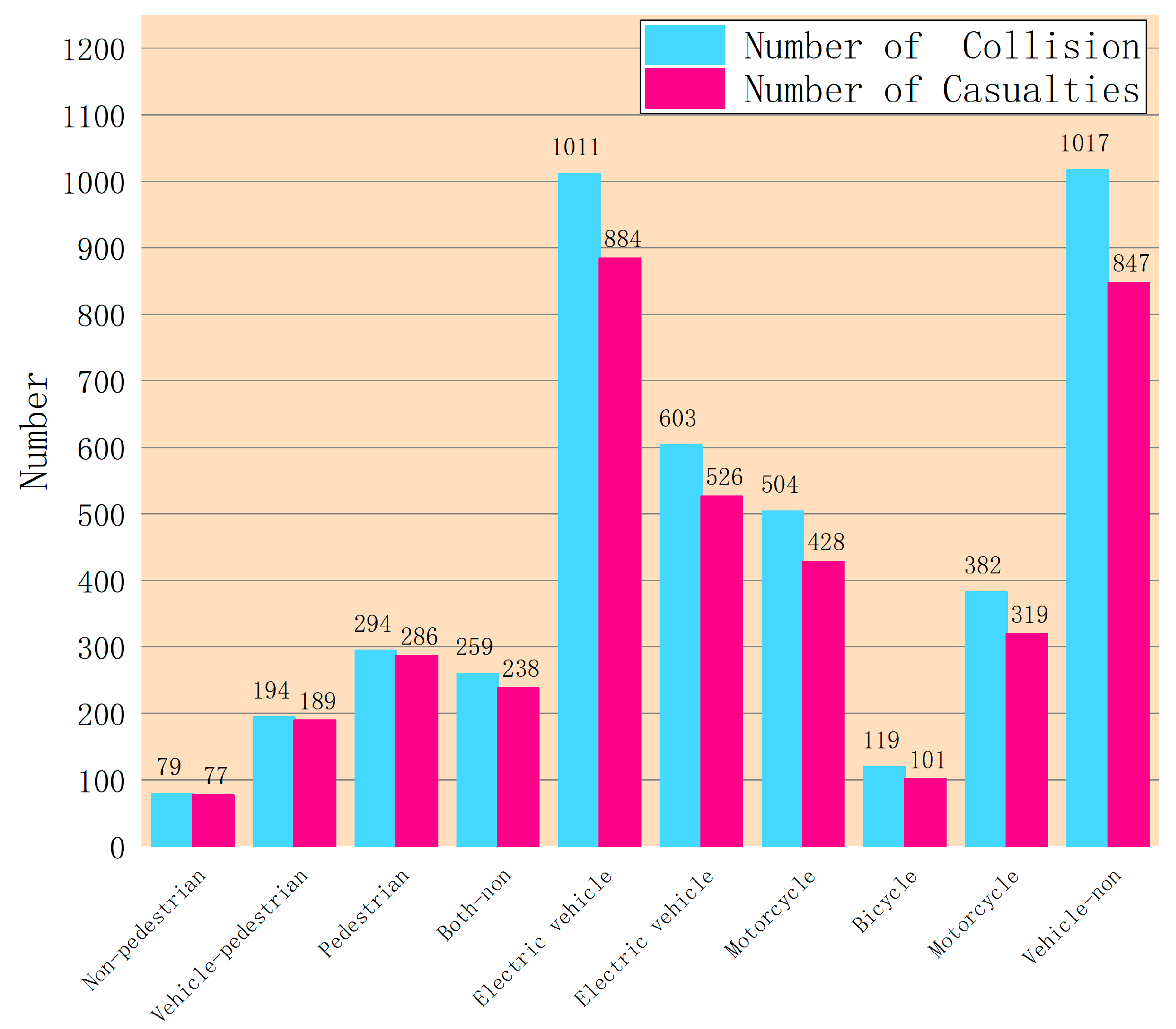
| Alarm Categories | Vehicle | 2212 | 632 | 28.57% |
| Vehicle-Non | 1017 | 847 | 83.28% | |
| Unilateral | 292 | 87 | 29.79% | |
| Vehicle-Pedestrian | 194 | 189 | 97.42% | |
| Non-Pedestrian | 79 | 77 | 97.47% | |
| Vehicle-Animal | 18 | 0 | 0% | |
| Both-Non | 259 | 238 | 91.89% | |
| Damage-Property | 1 | 0 | 0% | |
| Other | 213 | 46 | 21.60% | |
| Active Hit | Vehicle | 2106 | 900 | 42.74% |
| Pedestrian | 1 | 1 | 100% | |
| Electric-Vehicle | 603 | 526 | 87.23% | |
| Motorcycle | 382 | 319 | 83.51% | |
| Truck | 313 | 90 | 28.75% | |
| Small-Truck | 71 | 25 | 35.21% | |
| Big-Truck | 89 | 29 | 32.58% | |
| Bus | 75 | 27 | 36.00% | |
| Off-Road | 72 | 22 | 30.56% | |
| Van | 114 | 57 | 50.00% | |
| Taxi | 171 | 90 | 52.63% | |
| Bicycle | 36 | 26 | 72.22% | |
| Other | 252 | 4 | 1.59% | |
| Passive Hit | Vehicle | 1517 | 196 | 12.92% |
| Pedestrian | 294 | 286 | 97.28% | |
| Electric-Vehicle | 1011 | 884 | 87.44% | |
| Motorcycle | 504 | 428 | 84.92% | |
| Truck | 136 | 22 | 16.18% | |
| Small-Truck | 37 | 11 | 29.73% | |
| Big-Truck | 35 | 11 | 31.43% | |
| Animal | 26 | 0 | 0% | |
| Bus | 27 | 5 | 18.52% | |
| Bicycle | 119 | 101 | 84.87% | |
| Off-Road | 65 | 11 | 16.92% | |
| Taxi | 70 | 22 | 31.43% | |
| Van | 87 | 22 | 25.29% | |
| Other | 357 | 117 | 32.77% | |
| Collision Type | Crash | 2990 | 1647 | 55.08% |
| Dodge | 55 | 44 | 80.00% | |
| Rollover | 36 | 13 | 36.11% | |
| Scrape | 1015 | 346 | 34.09% | |
| Other | 118 | 59 | 50.00% | |
| Road Section | Prosperous | 3155 | 1559 | 49.41% |
| Non-Prosperous | 1130 | 557 | 49.29% | |
| Road Type | Straight | 2849 | 1418 | 49.77% |
| Crossroad | 1436 | 698 | 48.61% |
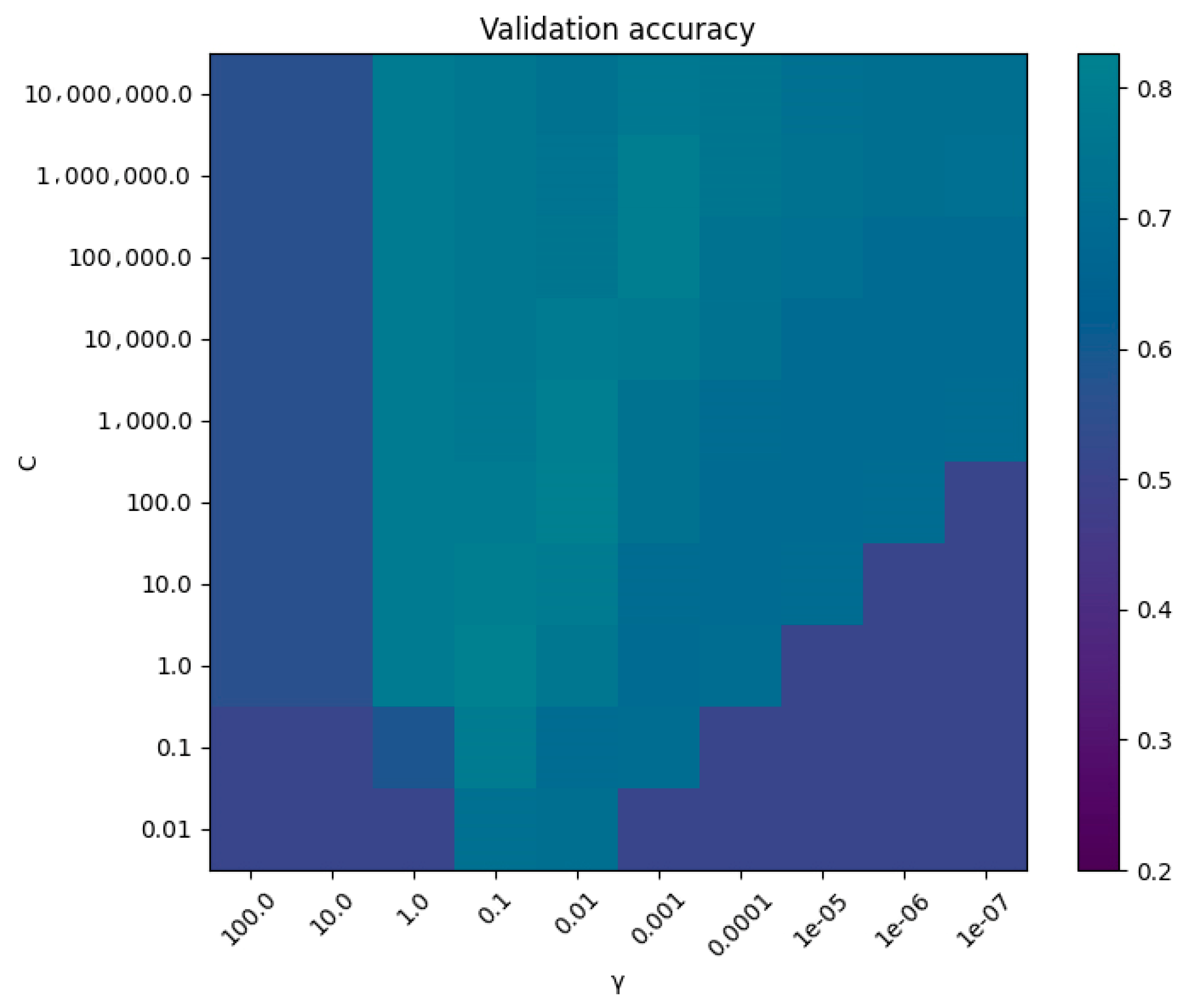
| C | γ | |
| GA-SVM | 87.2769 | 0.0481 |
| SSA-SVM | 1.1858 | 0.3559 |
| GWO-SVM | 146.8544 | 0.0127 |
| PSO-SVM | 1.194 | 0.3270 |
| Model | ACC | F1 | PRE | REC | MSE | AUC |
|---|---|---|---|---|---|---|
| SVM | 0.60 | 0.36 | 0.95 | 0.22 | 0.45 | 0.7324 |
| GA-SVM | 0.84 | 0.84 | 0.84 | 0.84 | 0.21 | 0.8856 |
| SSA-SVM | 0.86 | 0.86 | 0.93 | 0.85 | 0.16 | 0.8889 |
| GWO-SVM | 0.85 | 0.84 | 0.94 | 0.83 | 0.19 | 0.8799 |
| PSO-SVM | 0.85 | 0.85 | 0.93 | 0.84 | 0.16 | 0.8901 |
Disclaimer/Publisher’s Note: The statements, opinions and data contained in all publications are solely those of the individual author(s) and contributor(s) and not of MDPI and/or the editor(s). MDPI and/or the editor(s) disclaim responsibility for any injury to people or property resulting from any ideas, methods, instructions or products referred to in the content. |
© 2023 by the authors. Licensee MDPI, Basel, Switzerland. This article is an open access article distributed under the terms and conditions of the Creative Commons Attribution (CC BY) license (https://creativecommons.org/licenses/by/4.0/).
Share and Cite
Zhong, W.; Du, L. Predicting Traffic Casualties Using Support Vector Machines with Heuristic Algorithms: A Study Based on Collision Data of Urban Roads. Sustainability 2023, 15, 2944. https://doi.org/10.3390/su15042944
Zhong W, Du L. Predicting Traffic Casualties Using Support Vector Machines with Heuristic Algorithms: A Study Based on Collision Data of Urban Roads. Sustainability. 2023; 15(4):2944. https://doi.org/10.3390/su15042944
Chicago/Turabian StyleZhong, Weifan, and Lijing Du. 2023. "Predicting Traffic Casualties Using Support Vector Machines with Heuristic Algorithms: A Study Based on Collision Data of Urban Roads" Sustainability 15, no. 4: 2944. https://doi.org/10.3390/su15042944