A Voxelization Algorithm for Reconstructing mmWave Radar Point Cloud and an Application on Posture Classification for Low Energy Consumption Platform

Abstract

Applications for millimeter-wave (mmWave) radars have become increasingly popular in human activity recognition. Many researchers have combined radars with neural networks and gained a high performance on various applications. However, most of these studies feed the raw point cloud data directly into the networks, which can be unstable and inaccurate under certain circumstances. In this paper, we define a reliability measure of the point cloud data and design a novel voxelization algorithm to reconstruct the data. Experiments show that our algorithm can improve the stability of the point cloud generated from mmWave radars in terms of error reduction and scene re-construction. We demonstrate the effectiveness of our proposed algorithm using a neural network-based system for identifying a person’s sitting direction. In our experiment, compared with the baseline, our voxelization algorithm can improve the system in terms of accuracy (4.3%), training time (55.6%), and computational complexity, which is more suitable for light-weighted networks and low energy consumption platforms.

1. Introduction

Human activity recognition (HAR) is one of the most popular research topics in the literature. Combined with various sensor technologies and machine learning, a large number of HAR systems have been designed and applied in different applications. Camera-based systems [1,2,3] have been proven to own top-notch accuracy and outstanding resolution on posture detection and image identification. However, camera-based methods can have a low performance when used in the dark, smoke, or fog. Furthermore, these HAR systems have complex algorithms and time-consuming training processes, which entails a high resource cost. Therefore, to be able to detect in poor lighting conditions and for sustainable development, various types of low-cost sensors, such as radio frequency (RF) signal and WiFi signal transceivers, are utilized for HAR [4,5]. These sensors can detect and record changes in the environment caused by human activities. By processing and analyzing these signals, such systems can identify the corresponding human activities. For instance, Wang et al. [6] achieved basic human movement recognition using a WiFi signal. However, such a system has the disadvantages of overfitting issues which can lead to low accuracy in certain conditions [7]. Thus, researchers in [7] utilized data augmentation and a novel dense-LSTM model to prevent such problems and improve the performance. However, the robustness and resolution of these systems are insufficient for complex applications. Researchers in [8] utilized a C-band radar as a Doppler radar to classify six human activities. Since Doppler radars highly rely on the velocity information of the person, they are mostly used for moving posture classifications rather than stationary postures.

Thus, many researchers focus on the application of millimeter-wave (mmWave) radars to detect movement and stationary postures. This type of radar can work in the dark, fog, and smoke. It has a wide bandwidth of 4 GHz, which provides high-distance resolution. Moreover, the low cost also gives it a high potential in many fields. Therefore, many researchers utilized a mmWave radar as a 3D sensor for high-resolution applications. For instance, researchers in [9] proposed a system to identify and track people based on the point cloud provided by the mmWave radar. Furthermore, Singh et al. [10] combined the mmWave radar with CNN to classify stable human activities. These algorithms achieved high accuracy in identifying common activities, such as standing, sitting, or position tracking. However, challenges still exist for higher resolution posture estimation, as information embedded in the radar signal is prone to noise and hard to extract. Furthermore, the randomness of signal reflection and the limitation of the hardware make the point cloud unstable and it cannot provide an accurate understanding of the scene, as will be shown in Section 3. Moreover, the CNNs utilized in the aforementioned systems are too complex and not applicable for resource-limited platforms.

In this paper, we present a novel voxelization algorithm for processing the data from mmWave radars. We show that, although the point cloud provided by the radar can have a theoretically high accuracy in object detection, the traditional data processing chain is insufficient to extract the information and can lead to an unstable output, whereas an appropriate voxelization algorithm helps to solve the aforementioned problem and can re-construct the scene effectively. The algorithm is designed as a complementary algorithm. Instead of outperforming existing work in the literature, the objective of the proposed algorithm is to improve the stability of the data and to be inserted in the traditional processing chain of mmWave radars. To prove the advantages of our voxelization algorithms, we present a real-time system for recognizing the sitting direction of a human (facing front, back, left, or right), using a mmWave radar and a convolutional neural network (CNN). We compare the performance of the CNN with and without our voxelization algorithms. Different from many existing algorithms, including [11,12] which only used the positions of the detected points, or [13,14] which converted the point cloud to an image, our algorithm evaluates the reliability of the signal through its strength and features to filter out noise and emphasize the object of interest. We will show that our algorithm can reduce the training time of the network and increase the accuracy efficiently, while achieving a real-time processing time. Furthermore, with our voxelization algorithm, the system can use a light-weighted neural network for less energy and time consumption, which can help to reduce environmental pressures and promote sustainability in long-term development.

The contributions of this article can be summarized as follows:

• We show that, under certain circumstances, the results from commercial mmWave radars can be unstable and inaccurate when using only the traditional data processing chain.
• Considering the signal strength, features, and the positions of the points, we propose a novel voxelization algorithm to restore information in the scene effectively. Experiments show that our algorithm can reduce the error and re-construct a better scene.
• In our experiment, a CNN system for recognizing the sitting direction of a human with mmWave radars is presented. It proves that the proposed voxelization algorithm can effectively improve the feature representation of the data, resulting in improved network accuracy, reduced training time, and reduced network size for less energy consumption and sustainable development.

The rest of this article is arranged as follows. In Section 2, we discuss the relevant HAR algorithms in the literature. In Section 3, we introduce the preliminary knowledge about mmWave radars and highlight the problem of instability. In Section 4, we present our voxelization algorithm and CNN-based system. In Section 5, we evaluate the performance of our system in terms of accuracy, processing time, and training time. Section 6 concludes the work.

2. Related Work

HAR has been studied for decades. It includes, but is not limited to, human detection and tracking, action classification, and identification. It can be divided into three categories based on the device used in the systems: camera-based, wearable-device-based, and sensor-based methods.

Camera-based HAR has been studied in depth in the field of computer vision. For instance, Dalal et al. [15] proposed the histogram of oriented gradient descriptors to extract features from images manually, which can be applied to human detection. Researchers in [16] used a multi-camera vision system for detection and tracking people. However, such algorithms can merely detect relatively simple human activities. With the development of machine learning, neural networks can fulfil more complicated HAR tasks, such as posture estimation in complex environments. For example, Fang et al. [17] combined two neural networks (SSD-512 and ResNet-18) for regional multi-person pose estimation. Researchers in [18] utilized more complex neural networks (four decision models) on posture recognition for higher accuracy and more posture types. Moreover, Jalal et al. [19] combined the context-aware feature extraction approach with machine learning for sustainable event classification with higher accuracy.

However, the drawbacks of camera-based methods are apparent: cameras need good lighting conditions and have privacy concerns. The complex algorithms and neural networks make these systems inapplicable in low-energy-cost platforms and sustainable development [20,21]. Thus, some researchers proposed the use of wearable devices [22,23]. Wearable devices can be attached to a human and often have a wireless transceiver to transfer information to an embedded or removable processor, which can analyze the data and provide real-time feedback to the user. Various types of wearable devices have been applied in HAR, such as identification cards, GPS, and micromachined devices. For example, Cheng et al. [24] designed a flexible, textile capacitive sensor to recognize human activities. Some researchers also designed systems that combined multiple different wearable sensors, where each type of device can provide different information and be combined. For instance, Xia et al. [25] designed a falling detection system using accelerometers to detect a fall and GPS for the location information. However, these wearable device-based methods are not suitable for recognizing unauthorized people or for security applications. Furthermore, these methods have the risk that the devices may be lost or damaged.

Thus, some researchers choose sensors for HAR, such as WiFi signals, ultrasonic sensors, and Doppler radars. For instance, researchers in [26] utilized two Doppler sensors with a CNN to classify four motions. However, a Doppler radar highly relies on the velocity and has low performance when the target is stable. Furthermore, some researchers [27] utilized WiFi signal to generate a human activity model and recognize posture with improved linear discriminant analysis. However, Wu et al. [28] analyzed WiFi signals for human identification but they could not perform tracking simultaneously. mmWave radars, as a new type of sensor, have also been applied in HAR. In comparison with traditional wireless sensors such as WiFi, mmWave radars have a wider bandwidth of 4 GHz and a lower wavelength. These advantages enable mmWave radars to detect objects at a higher resolution and to be explored as a 3D sensor.

Thus, the applications of mmWave radars have become popular in HAR. For example, Cui et al. [11] used a two-radar system to detect and track people. Singh et al. [10] combined the mmWave radar with CNN to classify common human activities. However, most of the algorithms only focus on the position of the point cloud for denoising [29], while ignoring many other important factors, such as the signal strength and the reliability of the points. Specifically, they used clustering algorithms such as DBSCAN to eliminate noise and then fed the data into neural networks. Different from the point cloud produced by LIDARs, which has a large number of points with high reliability, the point clouds generated by mmWave radars have a smaller number of points with lower precision. It is much more difficult to select appropriate parameters for the clustering algorithms to distinguish noise from objects of interest. Furthermore, due to the lower angular resolution of mmWave radars when compared with LIDARs, data points from the stable object can become inaccurate and unstable, which is further explained in Section 3. Therefore, after the clustering process, there can still be a high proportion of unstable points remaining.

The voxelization algorithms for mmWave radars have not been studied thoroughly. In Sengupta et al. [13] and Jin et al. [14], researchers converted the point cloud into 3D images and fed the images into neural networks. However, because of the placement of the radars and the small number of points, information from the horizontal plane is much less dense than the vertical plane. Such voxelization algorithms can lead to a waste of computational power and a longer training and processing time. Furthermore, point cloud data often require an additional sampling step before being fed into a neural network. Such sampling algorithms are widely used in LIDARs. For instance, Schlomer et al. [30] used the farthest-point optimized point sampling algorithm to depict the point cloud efficiently. Moreover, Xu et al. [31] proposed the coverage-aware grid query algorithm, which improves the spatial coverage as well as reducing the time complexity. The sampling algorithms select the most important and representative points from the cloud in order to reduce the computational complexity and generate a fixed-size output that can be fed into neural networks. Although the point cloud from LIDARs is different from mmWave radars in terms of density and precision, we believe such algorithms would be beneficial in mmWave radar applications. Considering the fact that the point cloud from mmWave radars is generally smaller and more sparse, an appropriate up-sampling algorithm based on the reliability of the points can help the neural networks to extract the features and make decisions. Therefore, in this paper, we focus on the reliability of points to address the mentioned problems. We propose a novel voxelization algorithm which can be inserted into the traditional processing chain to re-construct the scene effectively. To demonstrate the effectiveness of the proposed algorithm, we apply it to detect the sitting direction of a person using mmWave radars.

3. Preliminaries and Challenges

In this paper, we utilize the TI IWR1443 mmWave radar which has the bandwidth of 4 GHz from 76 GHz to 81 GHz. The radar has four receivers and three transmitters. It can send a frequency-modulated continuous wave (FMCW) chirp signal, receive the reflection, and generate an intermediate frequency (IF) signal. The distance, velocity, and angle of the objects will be embedded in the IF signal. The on-chip processor then processes the range FFT, velocity FFT, and angle FFT, and uses the CFAR (constant false alarm rate) algorithm to give an output point cloud which includes the x, y, z position of each detected point. However, due to the limitation of the FFT resolution and the antenna layout, the output is not always as accurate as expected, as we will show in this section. The fundamentals of FMCW radars have been documented thoroughly in the literature, such as [11,32], so this section will only contain a brief description for understanding the mentioned issues.

3.1. Range FFT

In an FMCW radar model, an IF signal can be calculated from the transmitted signal and the received signal, which contains various frequency components that encode the distances between each object and the radar [32]. The range FFT is used to identify these frequency components. The resolution of the range FFT depends on the bandwidth of the radar, which is approximately 3.75 cm when using the full 4 GHz bandwidth available on the radar.

However, the result of the range FFT is also influenced by the distribution of the frequencies in the IF signal. As shown in Figure 1, assuming a person is standing stable 0.5 m away from a radar, we simulated the signal reflection from the body area from 0.5 m to 0.8 m with two different frequency distributions. In particular, the top figure shows when there is a signal reflection at every 0.01 m from the person, whereas the bottom one shows reflection at every 0.05 m. With a 3.75 cm range FFT resolution, the radar is able to distinguish the reflections separated at 5 cm as expected (as the peaks can be clearly seen in the bottom figure). However, frequencies with a closer distribution could result in a worse FFT resolution (as only two peaks are observed in the top figure). Although the reflections at 0.5 m and 0.55 m should be separable as the distance is larger than the theoretical resolution of the FFT, they become ambiguous when there are other reflections between them (0.51 m, 0.52 m, etc.). This effect is worse when considering the randomness of signal reflection, such as due to the angle of reflection and type of materials. Therefore, although the radar has a high theoretical distance resolution, the output can still be unstable and inaccurate.

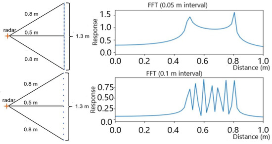
Figure 1. The result of the range FFT with different frequency components in the IF signal (0.01 m interval and 0.05 m interval, respectively).

3.2. Angle FFT

The radar has three transmitters and four receivers. It is able to determine the angle of arrival of a reflection by comparing the phase differences among the receivers [32]. To be specific, 8 virtual antennas are used to calculate the azimuth angle and 4 virtual antennas are used for elevation angle calculation. An angle FFT is used to calculate the angle of arrival of the object.

The resolution of the angle FFT depends on the number of antennas. With the TI mmWave radar used in our work, the angular resolution of objects in the front will be approximately 14°.

The angular resolution, again, can cause the instability of the output point cloud. In an experiment, we assumed there are three points approximately 1 m away from the radar and conducted a simulation. As shown in Figure 2, the left figure shows the scenario where the radar could only detect a single point that is 1 m away from the radar, because of the limited range resolution and angular resolution. However, if the points are rotated slightly (the right figure), then the radar will be able to detect the positions of these points correctly, as the distance between the points will become greater than 3.75 cm and become distinguishable in the range FFT. Therefore, a slight change in the scene could result in a significant change in the detected point cloud, which will be the main challenge for developing high robustness applications.

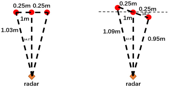
Figure 2. Example of unstable result caused by the range and angle FFT. (Left) the radar can detect only one point. (Right) the radar can detect all three points.

3.3. CFAR Peak Detection

The CFAR algorithm is used to detect the peaks from the FFT outputs. As the name states, this algorithm uses an adaptive threshold and aims to provide a constant false alarm rate for different signal strengths. Specifically, CFAR iterates through all data points and calculates the power of noise from the neighbouring cells. At any position, if the power of the point is higher than its neighbouring cells and the power–noise ratio is higher than a pre-defined threshold, this point will be considered as a peak (representing an object). Thus, besides the position (x, y, z) of each point, the radar can also provide the difference values between each peak value and their adjacent values. Unlike most of the mmWave algorithms which merely utilize the position of each point, the proposed method in this paper also considers the value from the CFAR algorithm and defines it as the reliability of the point, as will be shown in Section 4.3.

4. System Overview

In order to investigate the importance of the data reliability and necessity of an appropriate voxelization algorithm, we carried out a case study to determine the sitting posture of humans. Specifically, we let one person sit in an indoor environment with arbitrary postures, used one mmWave radar to monitor the person, and attempted to classify the sitting direction of the person (as shown in Figure 3).

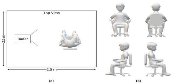
Figure 3. (a) Data collection using a single mmWave radar, with one person sitting in an empty room. (b) The four sitting directions to be classified.

4.1. Radar Configuration

In our experiment, we selected a set of signal configurations for an indoor environment, which has a maximum range of 6 m, a range resolution of 4 cm, a maximum speed of 1 m/s, and a velocity resolution of 0.1 m/s. We utilized the full 4 GHz bandwidth with a slope rate of 35 MHz/us. In order to keep as much information as possible from the raw data, we set the thresholds in CFAR to a relatively low value.

4.2. Dataset

Since there are few datasets of mmWave radars in HAR, we created a new dataset of point cloud graphs of humans sitting. We placed one TI IWR1443 mmWave radar on the sidewall at a height of 0.5 m. As shown in Figure 3, we let two people (one at a time) sit in an empty room in front of the radar, facing one of four directions (left, right, front, and back) with arbitrary postures. The radar was operated at 25 fps. For each time frame, we recorded the detected point clouds from the radar and calculated the reliability for each point. Every five adjacent frames were combined as one data sample, to emphasize the object of interest and reduce noise. There are approximately 5k samples in the dataset. Each sample is labelled manually with one of the four directions as the ground truth.

4.3. Reliability

As discussed earlier, we defined the reliability of a point to be the difference between its peak value and the adjacent values from the CFAR algorithm. Experiments show that approximately 10% of the points had a relatively high reliability value that can be up to 5 times higher than the rest. The large variance between the values and the imbalance of the data can negatively affect the training of a CNN, as the neural network may overfit to the large-scale values and ignore the others. Moreover, due to the instability of the radar signal and the imperfection of the data processing chain, the position variance of these large-weight points will be magnified into the network and lead to an incorrect result. On the other hand, as the reliability indicates the confidence in the position of the points, it is still necessary to feed this information into the network. Therefore, an appropriate data filtering and normalization scheme is required to train the network more effectively. Firstly, we converted the reliability into a logarithmic scale. Experiments showed that when training a neural network with raw values, the network hardly converges, whereas training with logarithmic values is much more effective. Then, based on the scaled reliability, we presented our voxelization algorithm.

4.4. Voxelization and Data Reconstruction

The data flow chart of our system is shown in Figure 4. Initially, we utilized the DBSCAN algorithm to cluster the points and extract objects of interest from the background. Since neural networks require a fixed-sized input, it is necessary to convert an arbitrary point cloud into a format that can be processed by the network. A typical process is voxelization, which divides a 3D volume into a discrete grid and regards each unit as one voxel. Considering that the resolution of the radar is approximately 5 cm, we sampled the input space into voxels at 5 cm × 5 cm × 5 cm. Then, we clustered all the detected points in the volume to the nearest voxel and calculated the sum of reliability for each voxel (as shown in Figure 5a). A voxel was classified as a point of interest if the voxel had several points attached to it or if it had high reliability. The reliability threshold was set to be half of the median reliability among all voxels. The rest of the voxels were classified as noise or unstable points, which were discarded (set to zero), as shown in Figure 5b. Once the data of interest were determined, we calculated the centroids of the point cloud and cut the graph to have a size of 150 cm × 150 cm × 150 cm from the centroids.

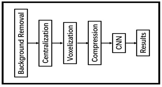
Figure 4. The diagram of our system.

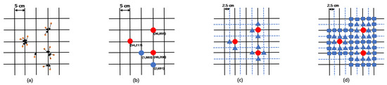
Figure 5. Illustration of the proposed algorithms. (a) Allocating the points to the nearest voxel. (b) Removing noise and unstable points based on the reliability of the points (red voxels are kept while blue voxels are discarded). (c) Splitting the remaining voxels based on the reliability (${\mathrm{V}}_2$). (d) Splitting the remaining voxels to a 5 × 5 square (${\mathrm{V}}_3$).

A traditional way of assigning voxel values would be a binary assignment, i.e., valid voxels will be assigned as one and the rest as zero. However, as we would like to embed the reliability into the graph, an advanced assignment rule is preferred. Taking the signal reliability and data size into consideration, we designed and compared three different voxelization algorithms. The baseline version (${\mathrm{V}}_1$) uses the reliability as the voxel values directly. It regards each 5 cm³ cube as a voxel, and the entire volume is cut into 30 × 30 × 30 voxels.

The following algorithms aim to increase the influence of useful points based on reliability. As we have shown in Section 3, when there is a set of closely located points, the radar may only detect a subset of them with a rather high amplitude. Therefore, instead of using a single value to represent the reliability, we chose to split each voxel based on the reliability, in order to reconstruct the information of the scene.

For the second algorithm (${\mathrm{V}}_2$), a voxel with high reliability will be split into two to six voxels based on the value so that a reliable voxel will gain more weight in the 3D graph and provide more spatial information. As shown in Figure 5c, we increased the resolution of the grid twofold along each dimension, and randomly distributed the new points around the original points. The reliability values of these new points are evenly divided based on the reliability of the original points. As a result, the reliability of the graph will be represented by both the reliability value and the point density. The graph’s resolution will increase twofold along each dimension, where each 2.5 cm³ cube represents one voxel, and the data size will be 60 × 60 × 60.

The third voxelization algorithm (${\mathrm{V}}_3$) uses the Gaussian distribution to split the points instead of randomly and evenly. We assume each detected point in the raw data represents a collection of points in the actual scene, where the distribution of these points follows a Gaussian distribution. Again, we doubled the resolution of the graph. Then, we defined a 5 × 5 × 1 Gaussian kernel (σ = 1) and performed a 3D convolution on the graph, as shown in Figure 5d. The resulting resolution and data size were the same as the ${\mathrm{V}}_2$ algorithm (2.5 cm³ and 60 × 60 × 60, respectively).

4.5. Data Compression

Since the mmWave signal reflects from the surface of the person, we found that information from the depth axis (z-axis) is often less precise and less dense than the vertical plane (x-y-axis). Therefore, in order to reduce the data size and the computational complexity, an additional compression step has been applied to the ${\mathrm{V}}_2$ and ${\mathrm{V}}_3$ algorithm. It compresses the data in the depth axis by combining every adjacent six frames. The resultant data size of ${\mathrm{V}}_2$ and ${\mathrm{V}}_3$ becomes 60 × 60 × 10, which is at a comparable level to the baseline algorithm.

As an experiment, we processed two sets of data with the ${\mathrm{V}}_3$ algorithm, one with the raw data (60 × 60 × 60) and the other with compressed data (60 × 60 × 10). We trained a neural network (details in the next section) on the two datasets, respectively, and the results are shown in Table 1.

Table 1. The accuracy, processing time, and training time of the compression experiments.

	Accuracy	Processing Time	Training Time
Raw data	98.3%	12.4 ms	4 iterations
Compressed data	98.5%	11.2 ms	4 iterations

We found that both datasets achieved a similar accuracy of approximately 98% and had a similar training time, which confirms the assumption that the majority of the features exist in the vertical plane (x-y-axis) rather than the depth plane. Compressing the data reduced the memory requirement to one-sixth of its original form and reduced the processing time by approximately 10%, to a comparable level with the baseline algorithm.

4.6. Neural Network Architecture

We designed three network architectures providing a trade-off between the network size and the performance. All the networks aim to classify four directions (facing front, back, left, and right). The details of architectures are shown in Table 2. Inspired by VGG-16 [33], we designed a six-layer CNN as the baseline model (L6) with three convolutional layers and three dense layers, a four-layer model (L4) with two convolutional layers and two dense layers, and a compressed four-layer model (L4C) with the same layer structures but only half the number of channels in each layer. Compared with the L6 model, the number of trainable parameters in L4 and L4C were reduced by approximately 61% and 90%, respectively.

Table 2. Network architectures.

Model Name:
L6	L4	L4C
Input:
30 × 30 × 30	60 × 60 × 10	60 × 60 × 10
Model Architecture:
ConV3-32 ConV3-64	ConV3-32	ConV3-16
Max-pooling
ConV3-128	ConV3-64	ConV3-32
Max-pooling
Dropout
FC-4096 FC-1024 FC-4	FC-1024 FC-4	FC-512 FC-4
Output: 4
Trainable Parameters:
38,022,180	14,810,020	3,705,812

We used the categorical cross entropy loss as the cost function:

$$\mathrm{loss}=-{{\displaystyle \sum }}_{\mathrm{i}=1}^{\mathrm{n}}{\hat{\mathrm{y}}}_{{\mathrm{i}}_1}{\mathrm{logy}}_{{\mathrm{i}}_1}+{\hat{\mathrm{y}}}_{{\mathrm{i}}_2}{\mathrm{logy}}_{{\mathrm{i}}_2}+\cdots +{\hat{\mathrm{y}}}_{{\mathrm{i}}_{\mathrm{m}}}{\mathrm{logy}}_{{\mathrm{i}}_{\mathrm{m}}},$$

(1)

where n and m are the numbers of samples and categories, y is the ground truth, and $\hat{\mathrm{y}}$ is the output from the network. We used the Adadelta optimizer [34] for the training, which uses a dynamic learning rate based on the frequency of weight change.

5. Evaluation

We processed our dataset with the proposed voxelization algorithms and trained the neural networks, respectively. An example of the processed point cloud with different algorithms is shown in Figure 6, where it can be seen that the ${\mathrm{V}}_3$ algorithm (the rightmost figure) shows the best visual effect in reconstructing the posture of the person. To show the effectiveness of our voxelization algorithm, we evaluated the performance of each algorithm in terms of the accuracy, the processing time, and the training time of the network (${\mathrm{V}}_1$ represents the traditional processing chain).

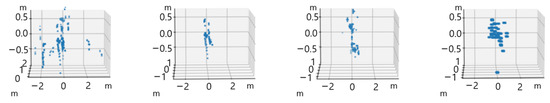
Figure 6. Examples of the point cloud when a person is sitting towards the right. From left to right, it shows the original point cloud and the processed point cloud from the baseline (${\mathrm{V}}_1$), ${\mathrm{V}}_2$, and ${\mathrm{V}}_3$ algorithm, respectively.

5.1. Accuracy

We define the accuracy as the percentage of the total number of correct predictions across all data. A comparison of the accuracy between the three voxelization algorithms is shown in Table 3. The result shows that, in all cases, the CNNs with an appropriate voxelization algorithm achieved the highest accuracy. In particular, for the L6 model, the accuracy of ${\mathrm{V}}_2$ and ${\mathrm{V}}_3$ is similar (all approximately 99%) and significantly higher than ${\mathrm{V}}_1$ (95.2%). This proves our assumption that although the DBSCAN algorithm can eliminate well-separated noise from clusters, it is insufficient in dealing with the instability within the data. However, this problem can be solved effectively through the proposed voxelization algorithms. By splitting and weighing the voxels based on their reliability, a better understanding of the scene can be obtained from the more reliable data points, which carry more significant features and help the training of the networks.

Table 3. Accuracy (in percentage) of the three system with different CNNs.

	L6	L4	L4C
${\mathrm{V}}_1$ (baseline)	0.952	0.932	0.874
${\mathrm{V}}_2$	0.994	0.968	0.961
${\mathrm{V}}_3$	0.995	0.987	0.985

Moreover, when the data are trained with the compressed model (L4C), it can be seen that the accuracy of ${\mathrm{V}}_2$ decreased to approximately 96%, while ${\mathrm{V}}_3$ still retained a high accuracy (approximately 98%), showing that the Gaussian distribution is more effective in reconstructing the scene from the raw data. The effectiveness of the ${\mathrm{V}}_3$ algorithm allows the use of a more light-weighted model with a reduced computational complexity and memory requirement, which is critical for low power consumption platforms and real-time applications.

5.2. Processing Time

We measured the inference time of each neural network on one point graph. All the experiments were carried out on a GeForce RTX 2060 GPU. The result is shown in Table 4. As the architecture of the networks is relatively simple, all models achieved a faster-than-real-time speed of more than 500 fps when taking advantage of a powerful GPU, and the compressed model can reach up to 1000 fps. The light-weighted networks make them possible to be ported onto low power consumption processors, such as digital signal processors, while retaining a high performance. In the meantime, the processing time of the voxelization algorithms varies from 7 ms to 10 ms on a CPU, which also satisfies the real-time requirement, and the delay can be negligible when the processing is pipelined. In a real-world application, the different combinations between the algorithms and the models provide a trade-off between the processing resource usage and the accuracy.

Table 4. Processing time of three different algorithms.

	Pre-Processing	L6	L4	L4C
${\mathrm{V}}_1$ (baseline)	7.13 ms	1.63 ms	1.12 ms	0.99 ms
${\mathrm{V}}_2$	9.92 ms	1.81 ms	1.33 ms	0.99 ms
${\mathrm{V}}_3$	10.20 ms	1.81 ms	1.33 ms	0.99 ms

5.3. Training Time

The networks were trained several times with the three different input formats. The experiment showed that networks trained with the ${\mathrm{V}}_3$ algorithms converge faster than the others while achieving the best accuracy, which confirms the assumption that the Gaussian distribution helps the network learn the scene. An example of the training process is shown in Figure 7. The second observation is that for the light-weighted L4C network, the training procedure for ${\mathrm{V}}_1$ takes approximately four times more iterations than the others while the accuracy is still lower, showing that an appropriate voxelization algorithm is more crucial for light-weighted networks and resource-limited platforms.

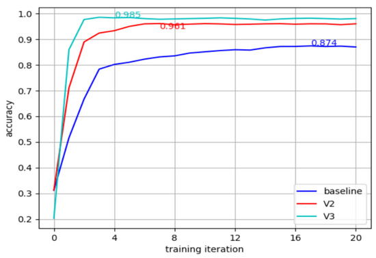
Figure 7. Training of the three algorithms in the L6 network.

5.4. Discussion

Based on the results shown above, we found that our voxelization algorithm is able to re-construct the scene effectively. To be specific, our voxelization algorithm helps to solve the unstable point cloud problem mentioned in Section 3, which results in higher accuracy in the detection of sitting direction. Furthermore, based on the reliability evaluation of voxels, the data processed by our system contain more significant features and have a better understanding of the scene. Thus, our system can utilize compressed light-weighted CNN, which provides the advantages of less training time, less processing time, and low energy consumption. We believe that this voxelization algorithm can be inserted into other mmWave systems, which can help to reduce energy consumption and boost sustainable development.

6. Conclusions

In this paper, we proposed a novel voxelization algorithm for mmWave radars. Different from most of the traditional algorithms which mainly focus on the distribution of the points, we defined the reliability for each point and used it to construct the voxels. Based on the characteristics of the point cloud produced by the mmWave radar, we proposed a few optimizations on the voxelization algorithm to reconstruct the point cloud, which emphasizes the reliable points and reduces the data size.

We showed that while the high resolution of mmWave radars enables us to perform complex HAR tasks, a suitable pre-processing algorithm can improve the performance and reduce the processing time and computational complexity. Our novel system can identify the sitting direction of humans with over 99% accuracy using lightweight CNNs. We showed that the proposed voxelization algorithm can effectively improve the feature representation of the data and results in improved accuracy and reduced training times on the same network. With the proposed algorithm, it is possible to achieve a similar performance with a 90% reduced network size, which is more suitable for power-limited sustainable platforms. A compressed model is also presented to provide a trade-off between the processing resource requirement and the accuracy to provide the sustainability of our system. As a complementary algorithm, we believe the proposed voxelization algorithms can be inserted and can benefit other applications in HAR fields with mmWave radars. In the future, we can optimize our algorithms to provide better compression and understanding of the scene, which cost less energy and are more suitable for sustainable development.

References

- Sun, K.; Xiao, B.; Liu, D.; Wang, J. Deep high-resolution representation learning for human pose estimation. In Proceedings of the IEEE/CVF Conference on Computer Vision and Pattern Recognition, Long Beach, CA, USA, 16–20 June 2019; pp. 5693–5703. [Google Scholar]
- Tian, Z.; Shen, C.; Chen, H.; He, T. Fcos: Fully convolutional one-stage object detection. In Proceedings of the IEEE/CVF International Conference on Computer Vision, Seoul, Republic of Korea, 27 October–2 November 2019; pp. 9627–9636. [Google Scholar]
- Wang, J.; Sun, K.; Cheng, T.; Jiang, B.; Deng, C.; Zhao, Y.; Liu, D.; Mu, Y.; Tan, M.; Wang, X.; et al. Deep high-resolution representation learning for visual recognition. IEEE Trans. Pattern Anal. Mach. Intell. 2020, 43, 3349–3364. [Google Scholar] [CrossRef]
- Ma, Y.; Zhou, G.; Wang, S. Wifi sensing with channel state information: A survey. ACM Comput. Surv. (CSUR) 2019, 52, 1–36. [Google Scholar] [CrossRef]
- Yan, H.; Zhang, Y.; Wang, Y.; Xu, K. Wiact: A passive wifi-based human activity recognition system. IEEE Sens. J. 2019, 20, 296–305. [Google Scholar] [CrossRef]
- Wang, F.; Gong, W.; Liu, J. On spatial diversity in wifibased human activity recognition: A deep learning-based approach. IEEE Internet Things J. 2018, 6, 2035–2047. [Google Scholar] [CrossRef]
- Zhang, J.; Wu, F.; Wei, B.; Zhang, Q.; Huang, H.; Shah, S.W.; Cheng, J. Data augmentation and dense-lstm for human activity recognition using wifi signal. IEEE Internet Things J. 2020, 8, 4628–4641. [Google Scholar] [CrossRef]
- Cadart, P.; Merlin, M.; Manfredi, G.; Fix, J.; Ren, C.; Hinostroza, I.; Letertre, T. Classification in c-band of doppler signatures of human activities in indoor environments. In Proceedings of the IET International Radar Conference (IET IRC 2020), Chongqing, China, 4–6 November 2020; Volume 2020, pp. 412–416. [Google Scholar]
- Zhao, P.; Lu, C.X.; Wang, J.; Chen, C.; Wang, W.; Trigoni, N.; Markham, A. mid: Tracking and identifying people with millimeter wave radar. In Proceedings of the 2019 15th International Conference on Distributed Computing in Sensor Systems (DCOSS), Santorini, Greece, 29–31 May 2019; pp. 33–40. [Google Scholar]
- Singh, A.D.; Sandha, S.S.; Garcia, L.; Srivastava, M. Radhar: Human activity recognition from point clouds generated through a millimeter-wave radar. In Proceedings of the 3rd ACM Workshop on Millimeter-wave Networks and Sensing Systems, Los Cabos, Mexico, 25 October 2019; pp. 51–56. [Google Scholar]
- Cui, H.; Dahnoun, N. High precision human detection and tracking using millimetre-wave radars. IEEE Aerosp. Electron. Syst. Mag. 2020, 36, 22–32. [Google Scholar] [CrossRef]
- Wu, J.; Cui, H.; Dahnoun, N. A novel high performance human detection, tracking and alarm system based on millimeter-wave radar. In Proceedings of the 2021 10th Mediterranean Conference on Embedded Computing (MECO), Budva, Montenegro, 7–10 June 2021; p. 20738335. [Google Scholar]
- Sengupta, A.; Jin, F.; Zhang, R.; Cao, S. Mm-pose: Real-time human skeletal posture estimation using mmwave radars and cnns. IEEE Sens. J. 2020, 20, 10032–10044. [Google Scholar] [CrossRef]
- Jin, F.; Zhang, R.; Sengupta, A.; Cao, S.; Hariri, S.; Agarwal, N.K.; Agarwal, S.K. Multiple patients behavior detection in real-time using mmwave radar and deep cnns. In Proceedings of the 2019 IEEE Radar Conference (RadarConf), Boston, MA, USA, 22–26 April 2019; pp. 1–6. [Google Scholar]
- Dalal, N.; Triggs, B. Histograms of oriented gradients for human detection. In Proceedings of the 2005 IEEE Computer Society Conference on Computer Vision and Pattern Recognition (CVPR’05), San Diego, CA, USA, 20–25 June 2005; Volume 1, pp. 886–893. [Google Scholar]
- Cucchiara, R.; Prati, A.; Vezzani, R. A multi-camera vision system for fall detection and alarm generation. Expert Syst. 2007, 24, 334–345. [Google Scholar] [CrossRef]
- Fang, H.-S.; Xie, S.; Tai, Y.-W.; Lu, C. Rmpe: Regional multi-person pose estimation. In Proceedings of the IEEE International Conference on Computer Vision, Venice, Italy, 22–29 October 2017; pp. 2334–2343. [Google Scholar]
- Ogundokun, R.O.; Maskeliūnas, R.; Damaševičius, R. Human posture detection using image augmentation and hyperparameter-optimized transfer learning algorithms. Appl. Sci. 2022, 12, 10156. [Google Scholar] [CrossRef]
- Jalal, A.; Akhtar, I.; Kim, K. Human posture estimation and sustainable events classification via pseudo-2d stick model and k-ary tree hashing. Sustainability 2020, 12, 9814. [Google Scholar] [CrossRef]
- Boz, Z.; Korhonen, V.; Koelsch Sand, C. Consumer considerations for the implementation of sustainable packaging: A review. Sustainability 2020, 12, 2192. [Google Scholar] [CrossRef]
- Kuhlman, T.; Farrington, J. What is sustainability? Sustainability 2010, 2, 3436–3448. [Google Scholar] [CrossRef]
- Mandal, S.; Turicchia, L.; Sarpeshkar, R. A low-power, battery-free tag for body sensor networks. IEEE Pervasive Comput. 2009, 9, 71–77. [Google Scholar] [CrossRef]
- Mukhopadhyay, S.C. Wearable sensors for human activity monitoring: A review. IEEE Sens. J. 2014, 15, 1321–1330. [Google Scholar] [CrossRef]
- Cheng, J.; Amft, O.; Bahle, G.; Lukowicz, P. Designing sensitive wearable capacitive sensors for activity recognition. IEEE Sens. J. 2013, 13, 3935–3947. [Google Scholar] [CrossRef]
- Xia, L.; Chen, C.-C.; Aggarwal, J.K. View invariant human action recognition using histograms of 3d joints. In Proceedings of the 2012 IEEE Computer Society Conference on Computer Vision and Pattern Recognition Workshops, Providence, RI, USA, 16–21 June 2012; pp. 20–27. [Google Scholar]
- Yang, Z.; Zhao, Y.; Yan, W. Adversarial vulnerability in doppler-based human activity recognition. In Proceedings of the 2020 International Joint Conference on Neural Networks (IJCNN), Glasgow, UK, 19–24 July 2020; pp. 1–7. [Google Scholar]
- Zuo, J.; Zhu, X.; Peng, Y.; Zhao, Z.; Wei, X.; Wang, X. A new method of posture recognition based on wifi signal. IEEE Commun. Lett. 2021, 25, 2564–2568. [Google Scholar] [CrossRef]
- Wu, F.; Zhao, H.; Zhao, Y.; Zhong, H. Development of a wearable-sensor-based fall detection system. Int. J. Telemed. Appl. 2015, 2015, 2. [Google Scholar] [CrossRef] [PubMed]
- Nickalls, D.; Wu, J.; Dahnoun, N. A real-time and high performance posture estimation system based on millimeter-wave radar. In Proceedings of the 2021 10th Mediterranean Conference on Embedded Computing (MECO), Budva, Montenegro, 7–10 June 2021; p. 21386661. [Google Scholar]
- Schlomer, T.; Heck, D.; Deussen, O. Farthest-point optimized point sets with maximized minimum distance. In Proceedings of the ACM SIGGRAPH Symposium on High Performance Graphics, Vancouver, BC, Canada, 5–7 August 2011; pp. 135–142. [Google Scholar]
- Xu, Q.; Sun, X.D.; Wu, C.-Y.; Wang, P.; Neumann, U. Grid-gcn for fast and scalable point cloud learning. In Proceedings of the IEEE/CVF Conference on Computer Vision and Pattern Recognition, Seattle, WA, USA, 13–19 June 2020; pp. 5661–5670. [Google Scholar]
- Iovescu, C.; Rao, S. The Fundamentals of Millimeter Wave Sensors; Texas Instruments: Dallas, TX, USA, 2017; pp. 1–8. [Google Scholar]
- Simonyan, K.; Zisserman, A. Very deep convolutional networks for large-scale image recognition. arXiv 2014, arXiv:1409.1556. [Google Scholar]
- Ruder, S. An overview of gradient descent optimization algorithms. arXiv 2016, arXiv:1609.04747. [Google Scholar]
Disclaimer/Publisher’s Note: The statements, opinions and data contained in all publications are solely those of the individual author(s) and contributor(s) and not of MDPI and/or the editor(s). MDPI and/or the editor(s) disclaim responsibility for any injury to people or property resulting from any ideas, methods, instructions or products referred to in the content. |
© 2023 by the authors. Licensee MDPI, Basel, Switzerland. This article is an open access article distributed under the terms and conditions of the Creative Commons Attribution (CC BY) license (https://creativecommons.org/licenses/by/4.0/).