1. Introduction
In the Monte Carlo modeling of neutron transport coupled with burnup calculations, one of the commonly evaluated parameters is power density. It is usually calculated in the specified fuel zones, called burnup zones or burnup regions. The zones are, in principle, the sets of the fuel assemblies, rods, or pellets in which the average neutron flux and reaction rates are calculated. The reaction rates are further used for calculations of isotopic changes in matter due to nuclear transmutations. The decay heat calculations are performed in line with calculations of nuclear transmutations. The decay heat is added to the power density. In such a way, the 3D map of power density distribution in the reactor core is obtained. The map can serve to present axial power density distributions for given radial burnup zones. Moreover, the power density distribution is used to calculate power factors,
Pf, defined as power density in a specified burnup zone relative to the average core power density. The
Pf are the final parameters because they present, in a straightforward manner, power density deviation from the average core power density [
1]. They are used to detect hot spots in the reactor core for further safety evaluation.
In the burnup problem, the calculations of power density are performed for arbitrarily defined time steps, e.g., the reactor cycle may be divided into time steps corresponding to one month, one week, or one day. Thus, the power density time evolutions in all burnup zones for given time points, are available. However, the evolutions are rarely investigated and shown. Usually, only the power density profiles for the beginning, middle, and end of the reactor cycle (BOC, MOC, EOC) are presented [
2]. In addition, the profiles show the average power density distribution in the reactor core without dividing them into particular axial and radial burnup zones. The calculation of exact step-by-step power density evolutions plays a crucial role in the detection of power density anomalies, understood as significant power density shifts along the active core. The obtained results may seem to be reliable and consistent with the predictions, but in principle, their compliance is a matter of chance.
Power density anomalies usually occur in the numerical modeling of nuclear systems with a thermal neutron spectrum, lack of axial symmetry, complicated fuel loading patterns, and quite long burnup steps. In thermal spectrum systems, such as pressurized water reactors (PWR) or high temperature reactors (HTR), the neutron flux coupling between burnup zones is weak, which means that the neutron field generated in one zone has a low influence on the neutron field in other zones [
3]. The size of the thermal reactors is usually larger than that of fast neutron reactors, which also promotes neutron flux decoupling. Additionally, power density anomalies cause spatial differences in the formation of
135Xe.
In turn, the non-uniform concentration of
135Xe causes further power density anomalies, which propagate with the reactor cycle. In thermal reactors,
135Xe significantly and criticality influences power density distribution due to a very large neutron capture cross-section of millions of barns. In fast nuclear reactors,
135Xe plays a negligible role due to a very low neutron capture cross-section in the fast energy range, below 1 barn. The power density anomalies may also be caused by the lack of geometrical symmetry of the numerical model. Usually, the numerical models developed for Monte Carlo simulations contain a reactor core surrounded by layers of side, top, and bottom reflectors. This approach is supported by the statement that the reactor core should be symmetrical, and the influence of the top and bottom reflectors are similar. However, the modeling of the reactor core at the level of the reactor pressurized vessel (RPV) introduces a lack of axial symmetry around the core. The effect may be especially observable above the active core, where the absorbing control rods are located. The effect is stronger when the operation of the control rods is modeled during the reactor cycle. Moreover, the complicated loading patterns of the reactor core are applied in all novel reactor systems. The core is loaded with many fuel assemblies of various types, as well as fuel enrichments. The assemblies are symmetrically distributed over the core. Additionally, some assemblies contain a gadolinia (Gd
2O
3) burnable absorber for long-term reactivity control. This causes difficulties in the numerical reconstruction of the reactor core and increases the number of burnup zones for power density calculations. In addition, the length of the burnup steps determines the formation of new isotopes during the burnup process. The isotopes with longer half-life time are less vulnerable to time step length, but bias in the spatial distribution of the short-lived fission products such as
135Xe may influence power density distribution [
4].
The problem of power density anomalies was investigated in some previous research [
5,
6,
7,
8,
9,
10,
11]. However, the detection of power density anomalies in coupled Monte Carlo and burnup modeling in a complex model of a full PWR reactor core enclosed in a reactor pressure vessel (RPV) was not found in the literature, and for this reason, it is presented in the current study.
Dufek and Hoogenboom have theoretically defined the problem of power density anomalies in critical reactor modeling using Monte Carlo codes [
5]. The additional works of Dufek et al. focused on the development of a novel stochastic implicit Euler method and a predictor-corrector method for coupled Monte Carlo neutron transport and burnup calculations [
6,
7]. In addition, the predictor-corrector schema was investigated by Isotalo and Aarnio [
8]. The issue of power density anomalies for high temperature thermal reactors was researched by Kępisty and Cetnar [
9]. The authors have applied different time step models for modeling PWR fuel assembly using 1D and 2D numerical models [
10]. In the papers, some alternative algorithms for power density calculations were proposed and tested. The effect of anomalies on axial power distribution in the simplified OPR1000 reactor model was investigated by Lee and Jung [
11]. The calculations of axial power profiles with thermo-hydraulic coupling for a large PWR reactor were shown by Li [
12]. The power distribution analysis, along with an analysis of the 24-month reactor cycle for the low-boron APR1400 core, were investigated by Do et al. [
13]. The comprehensive benchmarking studies on the APR1400 reactor core were performed by Barr et al. [
14]. The authors have compared results obtained using the deterministic MPACT code with reference results obtained with the Monte Carlo McCARD code for various numerical models. The results obtained with MPACT show very good agreement with the reference results, especially for reactivity and axial power distribution, which proves the reliability of the code.
The above-mentioned papers provide some background on the problems related to the power density calculations and anomalies in the PWR reactors in coupled neutron transport and burnup modeling. It is worth mentioning that the problem can be defined in various ways, not just for power density anomalies, but also for power density oscillations, power density instabilities, or power density asymmetry. However, all phenomena describe the same numerical effect of the non-uniform distribution of power density along the active core.
Section 2 shows the numerical setup used for the analysis, especially the applied tool, developed model, and performed calculations.
Section 3 presents the obtained results, i.e., power density distribution, power density time evolutions, and power density asymmetry in the core. In
Section 4, the obtained results are discussed and directions for future research are defined.
Section 5 concludes and summarizes the study.
2. Materials and Methods
2.1. Numerical System
The presented study was performed using the continuous energy Monte Carlo burnup code (MCB), designed for radiation transport and burnup calculations. The MCB code is the coupling of the well-known general Monte Carlo N-particle transport code (MCNP) for radiation transport and the trajectory transmutation analysis code (TTA) for burnup calculations [
15,
16]. Both codes were coupled at the level of the FORTRAN source code. MCNP subroutines are used to calculate neutron transport in any three-dimensional geometry of the numerical model. In practice, MCNP solves the neutron Boltzmann transport equation using the Monte Carlo methods. TTA is applied for calculations of isotopic changes in matter due to nuclear transmutations and radioactive decay [
17]. It solves the Bateman equations using the linear chain method, which is currently the reference method for burnup calculations. TTA uses the nuclear reaction rates calculated by the MCNP for power density and burnup calculations for every time step.
The MCB code calculates the isotopic changes in each material constituting a defined burnup zone. Initially, the neutron flux and spectrum are calculated using MCNP procedures developed for flux-based tallies. Then, power density is calculated using average recoverable energy per fission, or KERMA heating, and the volume of the burnup zone. In burnup calculation, the new material composition for subsequent neutron transport calculations is provided. The estimated decay heat is added to the calculated power density. The power density calculations are normalized to the user-provided total thermal power of the reactor. The power can change step by step, depending on the problem specification. The MCB uses a common beginning-of-step flux approximation, which assumes that neutron flux and reaction rates calculated at the beginning of the burnup step in the individual burnup zone are constant during the whole step.
In MCB modeling, it is possible to introduce geometrical changes to the numerical model during consecutive time steps. This approach facilitates the modeling of the control rod movement, or fuel shuffling. In addition, the sole change in the material composition for any predefined material can be also introduced. This functionality is commonly used for the adjustment of boric acid concentration (H
3BO
3) in the cooling water. MCB can use any transport libraries in the Evaluated Nuclear Data File (ENDF) format and is equipped with several libraries necessary for modeling isotopic changes in matter, e.g., energy-integrate nuclide formation ratios, fission product yields, metastable isotope formation probabilities, dose data, decay schemas, and others. The high-precision Monte Carlo modeling of neutron transport requires considerable computing power due to the nature of the neutron random walk and tallying processes. From the computing point of view, the demand for computer power increases with the complexity of numerical geometry, the number of burnup zones, and the time steps. Therefore, MCB has been equipped with the functionality of parallel calculations using the Message Passing Interface (MPI), which allows quite fast calculations with the usage of high performance computers (HPC). The MCB code was validated in the series of dedicated burnup calculations [
18].
2.2. Numerical Model
The numerical model was developed based on the available data for the Korean APR1400 reactor [
19,
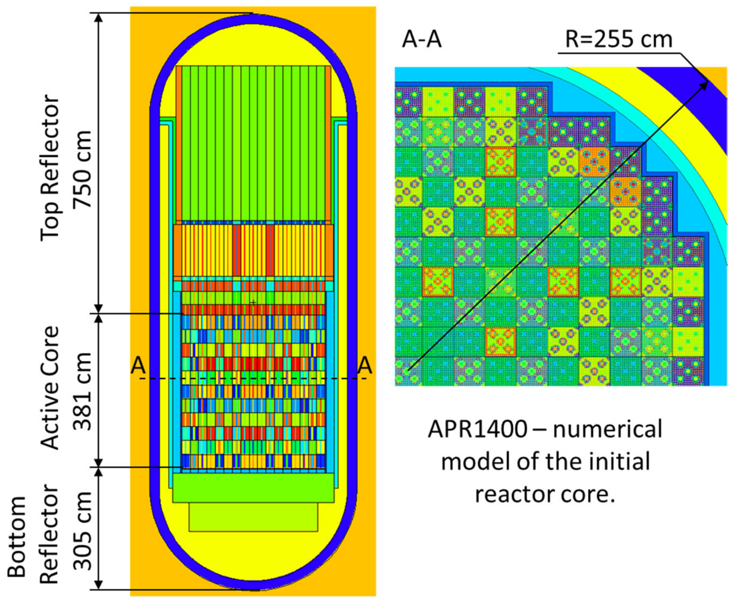
20]. The geometry of the reactor has been numerically reconstructed at the RPV level, considering the most important elements that may affect the neutron field in the reactor core, which is shown in
Figure 1. Unlike most numerical models for Monte Carlo simulations, the model is not only limited to the reactor core, top, bottom, and side reflectors, but also includes elements such as control rod banks located above the active core. The applied approach is more demanding when building a numerical model, as it requires the collection of an extensive set of input data, but it allows for more accurate numerical modeling [
21].
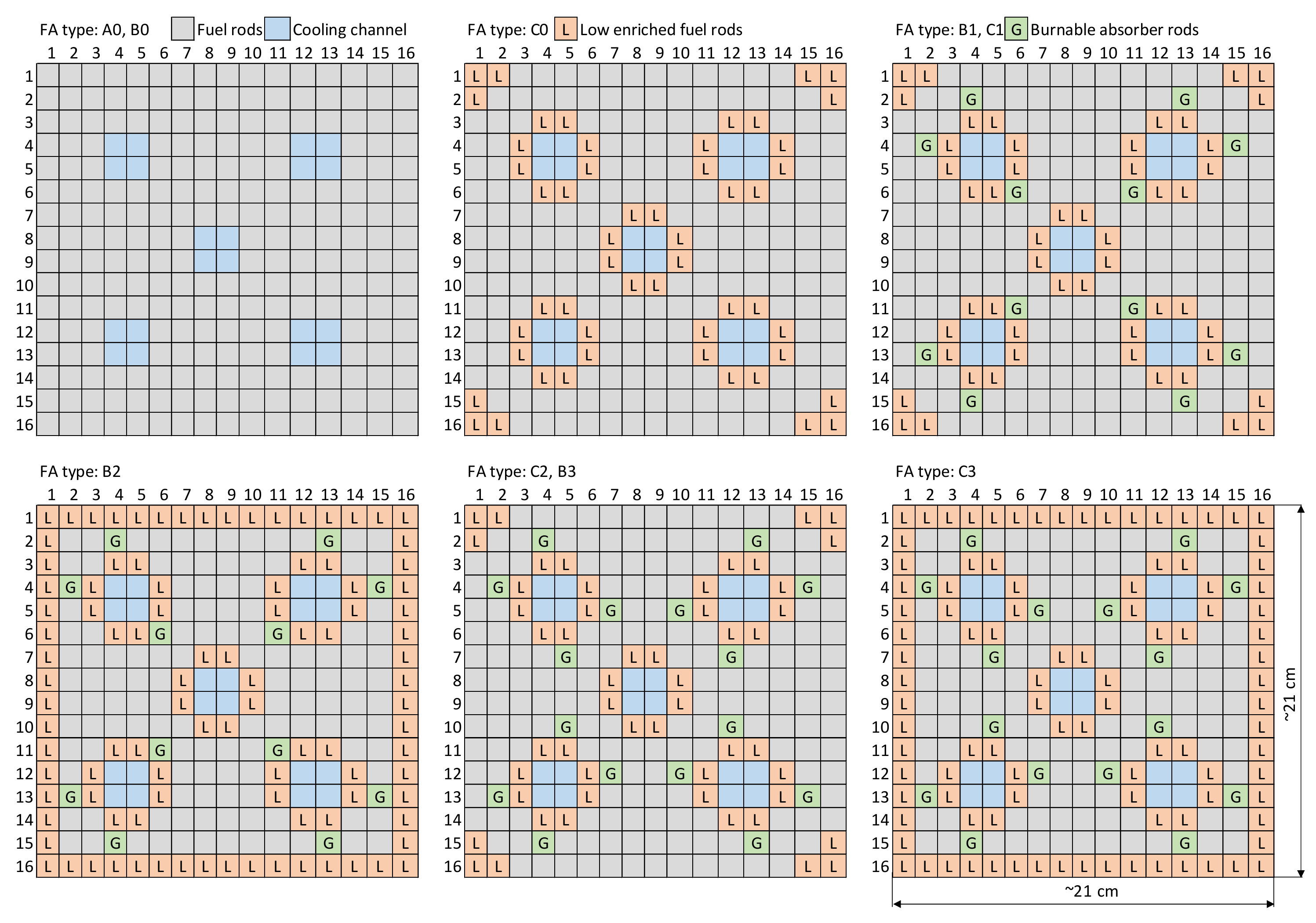
Table 1 shows the materials used for the numerical reconstruction of the reactor core elements. In the case of several elements with complex engineering shapes, the method of volumetric homogenization was used. It assumes the simplification of the geometry of the elements consisting of several materials by numerically creating one material having an isotopic composition corresponding to the volumetric fractions of the constituent materials. This method has been used mainly to reconstruct elements around the active core, consisting of coolant and steel components. The active core containing nuclear fuel was reconstructed in detail. Numerical modeling assumes that the initial reactor core is loaded with several types of fuel assemblies with different enrichments of nuclear fuel, as shown in
Figure 2 and
Figure 3. It is worth noting that the top and bottom ends of the burnable absorber rods located in some assemblies contain pure uranium fuel (UO
2) enriched to 2%
235U without a Gd
2O
3 absorber, which is also implemented in the numerical model. This design was introduced for increasing the power density at the peripheries of the core. In addition, the numerical model includes all banks of full- and part-strength control rods, as well as varying boric acid concentrations in the cooling water (H
3BO
3) [
22].
2.3. Numerical Modeling
The burnup and power density calculations must fulfill the assumed criteria defined by the model designer. These criteria are mainly related to the geometry of the burnup zones, reactor operating time, reactor power, and the use of reactivity control systems. An additional criterion is the precision of numerical calculations, defined by the number of neutron histories simulated in each time step, as well as the accuracy of the numerical procedures relevant to burnup calculations.
In the presented case of the APR1400 nuclear reactor, the rector’s core was divided into 242 burnup zones. The burnup zones were defined based on the type of fuel assemblies to be used in the initial reactor cycle, as well as the enrichment and type of nuclear fuel. In total, 22 radial burnup zones were defined. To obtain the axial power density distribution, all radial zones were divided into 11 uniform axial burnup zones.
Table 2 and
Table 3 show the divisions into radial burnup zones and the radially integrated initial mass of
235U.
The duration of the first reactor cycle was defined based on the desired final fuel average burnup of 17.571, provided in units of gigawatt-day per ton initial heavy metal (uranium) in the fresh nuclear fuel-GWd/tHMint. The time steps correspond to the time needed to reach the average burnup of 1 GWd/tHMint. The first step is shorter to determine the initial 135Xe concentration in the reactor core (~0.2 GWd/tHMint). The last time step is also shorter to achieve the final average burnup (~0.6 GWd/tHMint). Thus, the initial reactor cycle was divided into 20 burnup points, which yields a total of 19 burnup steps. During the first reactor cycle, the reactor works on a constant thermal power of 3983 MWth.
The reactivity control systems consist of control rods placed above the rector’s core, chemical shim (H3BO3), dissolved in the coolant, and a Gd2O3 burnable absorber in the uranium fuel. All these systems were included in the developed numerical model. The first APR1400 reactor cycle was designed without maneuvering the control rods. Thus, they have been placed above the active core and are stationary in numerical simulations. The concentration of boric acid in the coolant is determined at each time interval to maintain the core criticality. For this purpose, the functionality of the MCB, which allow for changing the isotopic composition of any material at any time step, was used. The effects related to Gd2O3 burnout have been included in the calculations. The calculations were performed using the Joint Evaluated Fission and Fusion 3.2 (JEFF) cross-section data libraries, in the kcode mode, for about 10 million neutron histories per time step.
The obtained power density is accompanied by the relative error defined as the estimated standard deviation of the mean power density divided by the estimated mean power density. The relative error is generated with four digits after the decimal mark. The calculations with a relative error of 0.1 (10%) are treated as generally reliable [
23]. Three intervals of relative error were introduced to show the precision of calculations: below 1%, between 1% and 1.5%, and between 1.5% and 2.5%. The relative errors in power density below 1% were obtained for 13 out of 22 axial burnup zones: A0, B0, C0N, C0L, B1N, B1L, C1N, B3N, B3L, C2N, C3N, C3N, and B3U-Gd. The relative errors between 1% and 1.5% were obtained for 6 out of 24 axial burnup zones: C1L, B2N, B2L, C2L, B1U-Gd, and C3U-Gd. The relative errors between 1.5% and 2.5% were obtained for 3 out of 24 axial burnup zones: B2U-Gd, C1U-Gd, and C2U-Gd. The highest relative error of 2.45% was obtained for the very top C1U-Gd burnup zone (indexed #1-T). The relative errors depend on the axial burnup zone position. The highest errors were obtained for the very top and bottom burnup zones due to lower neutron sampling. The difference between maximal relative errors (top or bottom burnup zone) and minimal relative errors (central zone) were analyzed. The difference for all pure uranium axial burnup zones is below 0.2%. The higher differences were observed for the gadolinia axial burnup zones, from about 0.3% to about 0.9%. The highest difference of 0.93% was observed for the C1U-Gd axial burnup zone. The low magnitude of the relative errors, much below 10%, proves that the precision of the Monte Carlo simulation is not the reason for the occurring power density anomalies, as shown in the following sections.
3. Results
3.1. Power Density Distribution
This section presents the power density profiles for the BOC, MOC, and EOC for all investigated burnup zones. The BOC corresponds to the fresh reactor core, the MOC to the average burnup of 9 GWd/tHMint, and the EOC to the final average burnup of 17.571 GWd/tHMint. The power factors Pf for each radial zone have been calculated in 11 axial burnup zones along the active core. The pure uranium axial burnup zones have the same length of 35 cm. The index “#1-T” corresponds to the first top burnup zone, index “#6-C” to the central burnup zone, and the index “#11-B” to the last bottom burnup zone. The Pf determines the ratio of the fuel power density in a given radial burnup zone to the average fuel power density of the reactor core—341 W/cm3.
Figure 4 shows power density profiles for burnup zones in the A0, B0, and C0 fuel assemblies. At BOC, the power density is lower in the zones adjacent to the top and bottom reflectors due to the neutron leakage outside the active core. The power density distribution in all burnup zones in the center of the core is almost flat, which is related to the applied design of the initial reactor core, particularly to the use of the burnable absorbers. The A0, B0, and C0 fuel assemblies, are adjacent to the fuel assemblies with a burnable absorber, which limits flux increase due to its burnout towards the center of the core, thus reducing the power density. In addition, B0 and C0 fuel assemblies are placed in the outer part of the active core directly adjacent to the side reflector, which also decreases the power density level, despite their higher enrichment.
In burnup zones for fuel assemblies containing burnable absorbers, i.e., B1-3 and C1-3, the power density profiles are almost flat along the entire height of the core, as shown in
Figure 5,
Figure 6 and
Figure 7 The applied burnable absorber rods contain pure uranium fuel enriched to 2% at the 30 cm top and bottom of the rod. The remaining central part of the rod is filled with UO
2 (92 wt. %) + Gd
2O
3 (8 wt. %) fuel pellets. The different design of the burnable absorber rods was included in the numerical model by a slight height modification of the peripheral top and bottom burnup zones. This approach provides a mechanism for the power drop compensation near the top and bottom reflectors in all assemblies due to the lack of power damping by Gd
2O
3 and the power increase due to a higher mass of
235U and fuel enrichment. The effect is observable in
Figure 8 and
Figure 9, which show the power density profiles in burnup zones representing rods with a burnable absorber. In all cases, the maximal
Pf is slightly larger than 1.2 at BOC.
The power density profiles at MOC for all burnup zones present the peak in the center of the active core. The formation of a central peak is related to the faster burnout of the burnable absorber in the middle of the core, which extends to the neutron flux and power increase. The maximal Pf of about 1.6 was observed in burnup zones C2 and C3, which have the highest enrichments and are located in the center of the core.
The power profiles at the EOC for all burnup zones show the large peak for the second axial burnup zone (#2) near the top reflector. The maximal Pf of about 1.8 at EOC were obtained for zone C3, with the highest enrichment. Theoretically, the power profiles should show two similar peaks near the top and bottom reflector and decrease at the active core’s middle. The analytical shape is related to the highest fuel depletion in the center of the core, causing a power drop. Therefore, the compensation of total core power is driven by enhanced burnup near to the top and bottom reflectors and the power increase in these regions. The regular behavior is, to some extent, only observable at EOC. Contrary to the shapes of power profiles at BOC and MOC, the shape at EOC shows irregular behavior.
The behavior is likely a sign of power density anomaly in the numerical modeling near the end of the reactor cycle, which is investigated in the following sections.
3.2. Power Density Evolution
Further investigation of the irregular behavior of the power profiles considers analyses of Pf time evolution in the chosen burnup zones. In the analyses, the Pf evolutions of both the pure uranium and burnable absorber zones are considered. The developed zoning schema of the reactor core into an odd number of axial burnup zones allows for the time analysis of the power evolution in the significant location in the active core. The first investigated axial zone (#6-C) is located at the very center of the active core. The second investigated axial zone (#11-T) is located at the very bottom of the active core near the bottom reflector. The third investigated axial zone (#1-T) is located at the very top of the active core near the top reflector and control rods. The burnable absorber is not present in the top and bottom zones (#1-T and #11-B); thus, the second from the bottom (#10) and second from the top (#2) axial burnup zones were also considered in the analysis.
For all the burnup zones, Pf evolutions can be classified into their types. The radial zones B1, B3 and C2, C3 show the highest power density, zones A0, C1, and B2 show medium power density, and zones B0 and C0 show the lowest power density. The power level depends on the fuel enrichment and the location of the zone in the reactor core.
Figure 10 presents the
Pf evolutions in the pure uranium central axial burnup zones. The curves show a characteristic peak at 9 GWd/tHM
int and a tail at 12 GWd/tHM
int for all burnup zones (#6-C). The maximum peak in
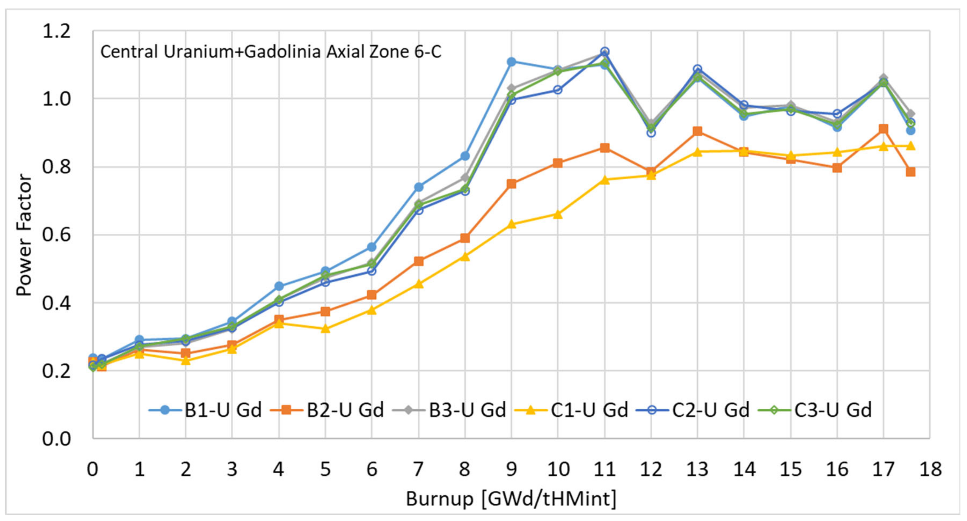
Pf of about 1.6 was observed for high power zones. The peaks correspond to the almost full burnout of the gadolinium isotopes in the core center and the subsequent increase in neutron flux. The formation of the tail is related to the power shift from the center of the core to the top and bottom. The power evolution for the medium power zones shows more stable behavior during the reactor cycle. However, a power decrease in the lower power zones was observed. This effect is related to the placement of the zones at the radial core peripheries and thus, a decrease in neutron flux due to neutron leakage and fuel depletion. In the Gd
2O
3 bearing axial burnup zones, the power increases in the function of Gd burnup and reaches maximum at 9–11 GWd/tHM
int, which corresponds to
Pf of 1.1, for high power zones. Afterward, the behavior of
Pf is similar to that of the pure uranium burnup zones, see
Figure 11.
Figure 12 shows the
Pf evolutions for the bottom pure uranium fuel zones (#11-B). The highest
Pf of about 1.4 was observed at BOC for the fresh reactor core. The magnitude of the
Pf is lower compared with the central axial zones. The
Pf decreased continuously to about 9–10 GWd/tHM
int, which corresponds to the power shift towards the reactor center due to the Gd burnout. Next,
Pf starts to increase to about 12–13 GWd/tHM
int due to a power drop in the center and compensation at the core peripheries. The power anomalies occur at 14 GWd/tHM
int. From this point,
Pf presents fluctuant behavior, with a maximal
Pf of about 1.2 at 17 GWd/tHM
int. The power evolutions in the bottom parts of the burnable absorber zones, which contain only pure uranium fuel, are similar to the power evolutions in other pure uranium zones. The maximal
Pf equals about 0.9 for the peak at 17 GWd/tHM
int, which is shown in
Figure 13. It is worth noting that the initial
Pf for the fresh core drops significantly in the second time step after the formation of absorbing fission products.
Pf time evolutions in the second from the bottom axial burnup zones (#10) show a more stable behavior compared with the very bottom burnup zone, as presented in
Figure 14. The power profiles are flatter, and the tail at 9–10 GWd/tHM
int is smaller. However, the peaks have a greater amplitude, with a maximal
Pf of about 1.7 at 15 GWd/tHM
int. The power evolution in the burnable absorber burnup zones shows similar behavior as that in the central fuel zone, see
Figure 15. However, the power increase is smoother due to the slower Gd burnout until about 13 GWd/tHM
int. The maximal
Pf equals about 1.4 for the peak at 15 GWd/tHM
int. The initial drop in
Pf is observable.
Figure 16 shows the evolutions of
Pf in the very top axial burnup zones (#1-C) adjacent to the top reflector. Likewise, in the bottom burnup zones, the power drop in the middle of the reactor cycle is observable. However, the curves present the anomalies in
Pf, practically from the beginning of the reactor’s cycle. The anomalies demonstrate a regular character, showing increases and decreases every single time step from about 5 GWd/tHM
int. Additionally, at approximately 9 GWd/tHM
int, the amplitude starts to increase from cycle to cycle. The maximal
Pf is about 1.4 for the EOC. Similar behavior of
Pf is seen in burnup zones containing burnable absorbers (see
Figure 17). In this case, the maximum
Pf is also about 1.0 for EOC. There is an observable increase in power density after the first time step.
Figure 18 shows the
Pf evolutions in the second from the top axial pure uranium burnup zones. The behavior of the curves is similar to that in the very top burnup zone in relation to power density anomalies. The maximal
Pf equals about 1.8 at EOC. The curves do not present a significant power drop at MOC, similar to the behavior in the second from the bottom axial burnup zone. The power increases in the second burnup step. The
Pf in the burnable absorber burnup zones increases from BOC to about 12 GWd/tHM
int (see
Figure 19). The power anomalies are visible from about 5 GWd/tHM
int. The maximal
Pf of about 1.4 was observed for EOC.
In further analysis, the axial power density asymmetry along the active core is considered. The approach allows for easy detection and quantification of the power density anomalies.
3.3. Power Density Anomaly Detection
The power asymmetry factor PAS was defined as the ratio of the power density in any top axial burnup zone to the symmetrical bottom burnup zone. The PAS has been calculated for all radial pure uranium and burnable absorber burnup zones. The factor allows for the detection of power density anomalies along the active core for a given reactor cycle length. The PAS values around unity show a symmetrical distribution of the power density along the active core. The anomalies correspond to the PAS factor far from unity, which shows the significant power density shifts towards reactor core peripheries. The PAS presents power density anomalies in a straightforward manner; however, its application demands the development of a high-resolution numerical model with the axial core division into at least a few burnup zones.
Figure 20 presents the
PAS factor for the initial reactor cycle in two axial burnup zones above (#5) and below (#7), as the central burnup zone (#6-C). It can be noted that up to about 11 GWd/tHM
int, the maximal deviation of the
PAS factors from unity is about 10%, but in most cases, it is much smaller. After 11–12 GWd/tHM
int, clear increases and decreases in
PAS are visible, which shows the asymmetry—and thus, the anomaly—of the power density distribution. The maximum deviations are about 20%. Similar behavior of the factors is observable for the pure uranium and burnable absorber burnup zones.
The
PAS factors for the four consecutive burnup zones at the top (zones #1-T and #2) and bottom (zones #11-B and #10) of the active core are taken into account. Such an approach allows for a cautious analysis of the anomalies along the active core.
Figure 20 also shows that regardless of the type of burnup zones, the
PAS anomalies occur practically from the beginning of the reactor cycle. The anomalies show the largest
PAS of about 1.8 after 11 GWd/tHM
int, and their amplitude increases with time. Anomalies for the outer zones directly adjacent to the reflector show a larger amplitude. The behavior of the
PAS factors in the peripheral zones indicates a large asymmetry of the power density distribution, especially at the end of the reactor cycle. The genesis of the numerical effect is discussed in the following section.
4. Discussion
The obtained results show the numerical anomalies in the axial power density distribution in the APR1400 rector’s core numerical model. The anomalies are observable in the time and spatial domains of numerical modeling. The largest anomalies were observed in the axial burnup zones located on the peripheries of the active core at the top and bottom reflectors at the end of the initial reactor cycle.
A major effect causing power density anomalies in coupled Monte Carlo neutron transport and burnup calculations is the difference in the initial neutron flux due to different designs of the top and bottom reflectors. In the presented numerical model, the control rod banks are located above the active core, which increases neutron absorptions in the top regions. Thus, initial neutron flux and power density are lower in the top zones and higher in the bottom zones. This initial flux asymmetry initiates the formation of further power density shifts and finally, strong anomalies. In the second calculation step, the power increases significantly in the top zones and decreases in the bottom zones. The effect is strictly related to the formation of absorbing 135Xe. The concentration of 135Xe in the top burnup zones is lower because of the lower initial power density. On the contrary, in the bottom burnup zones, the initial power density is higher, causing a larger production of 135Xe. In general, the differences in power density along the active core extend to the different formation rates of absorbing 135Xe and subsequent asymmetric power density distribution in the next irradiation step. The effect propagates with burnup.
The
135Xe distribution is shown in
Figure 21 in the form of the
135Xe asymmetry factor, defined as the ratio of
135Xe concentration in the subsequent top burnup zone to the
135Xe concentration in the subsequent bottom burnup zone. The
135Xe asymmetry factor time evolutions are shown for the same zones as for the
PAS factors. The plots show strict relationships between power shifts and
135Xe distribution along the active core. The high power density corresponds to the low concentration of
135Xe, and the low power density corresponds to the high concentration of
135Xe.
The anomalies in the top axial burnup zones occur faster from about 5 GWd/tHMint because of the additional absorptions in control rod material and the associated significant power density changes. The presence of anomalies in the center and bottom of the reactor core from about 14 GWd/tHMint is related to the burnout of the gadolinium burnable absorber, and thus, faster fuel depletion, resulting in significant power density shifts to the core peripheries. The power density shifts coincide with the initial power anomalies caused by the core asymmetry, which extends to the increase in their amplitude at the EOC. Thus, in regards to EOC, 135Xe begins to be the leading absorbing isotope, with a large influence on neutron flux distribution and power density. From the above, it can be determined that the numerical problem of power density anomalies mainly depends on the concentration of 135Xe having a large neutron absorption cross-section.
Future research will focus on the three significant areas related to the detection, interpretation, and finally, the prevention of power density anomalies. First, a more detailed modeling of the initial reactor cycle, with a larger number of burnup steps and zones, will be implemented for the parametric study. Second, the influence of control rod modeling on power density anomalies will be investigated. Third, the interactions between all absorbing isotopes for a given burnup and their influence on power density distribution will be analyzed. All these issues make the analysis more challenging in terms of developed numerical apparatus and computer power demand, but will allow for more reliable modeling of the reactor core.


