Prediction of Carbon Emission of the Transportation Sector in Jiangsu Province-Regression Prediction Model Based on GA-SVM

Abstract

To meet the twin carbon goals of “carbon peak” and “carbon neutrality”, it is crucial to make scientific predictions about carbon emissions in the transportation sector. The following eight factors were chosen as effect indicators: population size, GDP per capita, civil vehicle ownership, passenger and freight turnover, urbanization rate, industry structure, and carbon emission intensity. Based on the pertinent data from 2002 to 2020, a support vector machine model, improved by a genetic algorithm (GA-SVM), was created to predict the carbon peak time under three distinct scenarios. The penalty factor $c$ and kernel function parameter $g$ of the support vector machine model were each optimized using a genetic algorithm, a particle swarm algorithm, and a whale optimization algorithm. The results indicate that the genetic algorithm vector machine prediction model outperforms the particle swarm algorithm vector machine model and the whale optimization vector machine. As a result, the model integrating the support vector machine and genetic algorithm can more precisely predict carbon emissions and the peak time for carbon in Jiangsu province.

1. Introduction

Climate change is a global problem that impacts human survival and destiny. The greenhouse effect brought on by carbon emissions is one of several essential variables contributing to climate change. As the world economy expands quickly, carbon dioxide gas is emitted into the atmosphere due to the extensive use of industrial fuels, including coal, oil, and natural gas. The atmosphere’s invisible, transparent barrier of carbon dioxide gas absorbs heat rays from the Sun while preventing the Earth’s heat from escaping into space, warming the planet’s climate. Scientists predict that if the trend in surface temperature continues, the world’s temperature will rise by 2–4 degrees Celsius by 2050 [1], the North and South Polar icebergs will melt significantly, raising sea levels significantly, and some island nations and coastal cities will be submerged in water. Other secondary disasters, including an increase in pests and diseases, the EI Niño Phenomenon [2], increased ocean storms, land droughts, and a rise in desertification, will be associated with this.

On 22 September 2020, the Chinese government proposed that “China will increase its independent national contribution, adopt more aggressive policies and measures, strive to peak CO₂ emissions by 2030, and strive to achieve carbon neutrality by 2060” at the 75th session of the United Nations General Assembly. The adoption of total carbon emission prediction and control in the transportation industry is an inevitable consequence of energy saving and carbon reduction in the transportation industry. It represents the third largest source of carbon emissions [3].

In recent research on transportation carbon emissions, scholars have focused on three areas: factors influencing transportation carbon emissions, the prediction of transportation carbon emissions, and the control of transportation carbon emissions. There are models such as gray prediction, improved regression, and machine learning in the long-term forecast.

In terms of gray prediction, Pao et al. (2011) [4] studied Brazilian carbon emissions from 1980 to 2007 and predicted the carbon emissions from 2008 to 2013 using a gray prediction model (GM). The MAPE value of this prediction model is less than 3%. Huang et al. (2022) [5] proposed a nonlinear multivariate gray model (ENGM (1,4)) based on the environmental Kuznets curve (EKC) and adopted particle swarm for optimization; the MAPE value of this prediction model reached 0.6025%. The accuracy of such models is generally not high without algorithmic improvement.

With the rise of various machine learning algorithms, machine learning forecasting is also popular; for example, Sun et al. (2017) [6] used the particle swarm optimization (PSO) algorithm to optimize the extreme learning machine and used it to predict carbon emissions in Hebei province, China. Hong et al. (2018) [7] used a genetic algorithm to predict the carbon emissions of the Korean construction industry in 2030, with a MAPE value of 2.06%. Wen et al. (2020) [8] optimized the parameters in the BP neural network model by particle swarm to improve the prediction accuracy further. The MAPE figure reached 1.27%. The biggest drawback of this modeling approach is that the statistical sample has to be large enough and that it requires sufficiently accurate raw data.

In improved regression, Fang et al. (2018) [9] used a particle swarm-improved Gaussian process regression method, which can effectively optimize the hyperparameters of the covariance function in Gaussian process regression. The improved Gaussian process regression method improved the prediction accuracy of the original GPR method and outperformed other traditional prediction methods with a MAPE figure of 2.74421%. Using a lion swarm optimizer and a genetic algorithm, Qiao et al. (2020) [10] optimized a conventional least squares support vector machine model. The MAPE value of the new model was reduced to 0.726–1.878%. The vector machine model does not require large data samples and outperforms neural networks for small samples of carbon emissions with higher accuracy than gray prediction [11]. Flaws, such as easily plunging into local optimum, over-fitting, and poor generalization capability, remain. Then, a genetic algorithm is needed to improve it.

In summary, the novelty of this study is that, starting from the STIRPAT model, which affects multiple factors of carbon emissions, the data are first processed by partial least squares (PLS) [12] based on the possible covariance of the data, which ensures the operability of the data. To improve the prediction accuracy of the support vector machine and prevent it from entering the optimal local solution, its parameters are improved with a genetic algorithm. The new model combines multiple methods with multiple features that allow for predicting carbon emissions with high accuracy and flexibility. It considers complex influencing factors and provides new ideas and methods for the medium- and long-term prediction of carbon emissions.

2. Materials and Methods

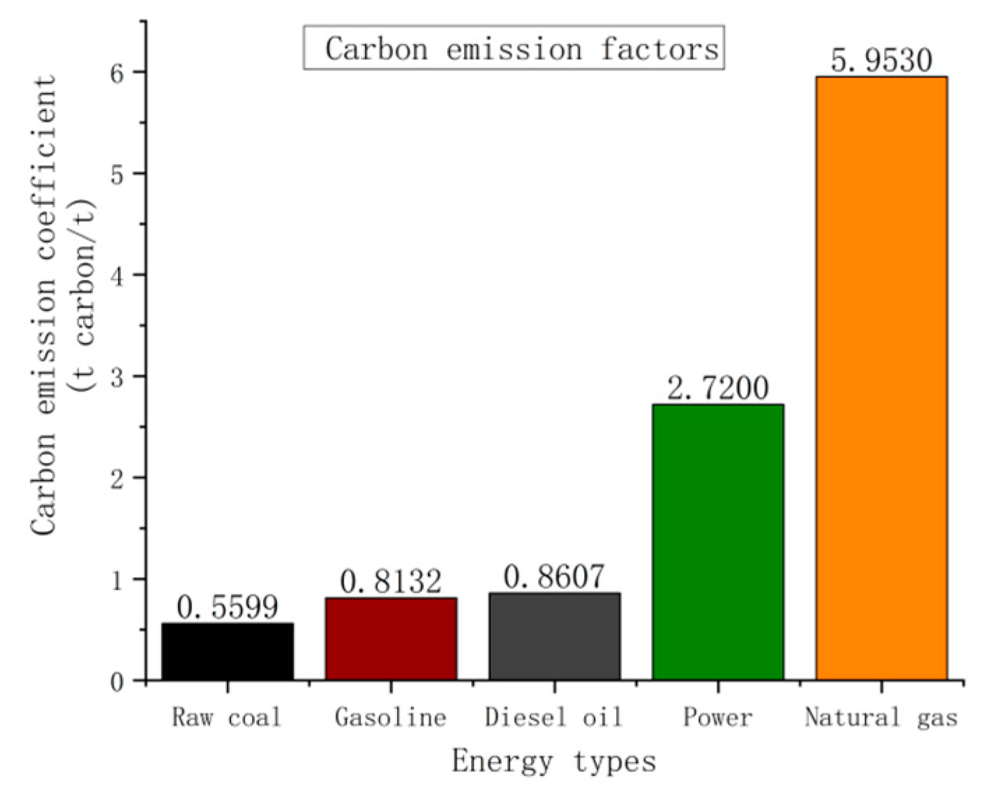
2.1. Establishment of Transportation Carbon Emission Measurement Model

Direct and indirect carbon emissions make up the overall industry’s emissions. Direct emissions refer to the greenhouse gas emissions generated by the burning activities of fossil fuels such as coal, natural gas, and oil, and industrial production processes; indirect emissions are emissions that result from the actions of an enterprise but occur at sources owned or controlled by other enterprises. Its testing model primarily considers direct carbon emissions due to the unique characteristics of transportation carbon emissions.

In 1971, Ehrlich and Holden proposed the IPAT model [13], which suggested that the total carbon emissions were related to the entire population, GDP per capita, and energy consumption intensity. In 1989, Kaya Yoichi proposed the Kaya model [14], which added a fourth influence factor of carbon emissions per unit of energy consumption to the IPAT model. In 1994, York and Dietz proposed the STIR model [15], which suggested that various factors should affect carbon emissions in a nonlinear relationship; the influencing factors were population, economy, and technology. In 2007, Ang et al. [16] proposed the LMDI model, which suggested that industrial structure also affects carbon emissions.

Referring to the STIRPAT model and the research results of Zhang et al. (2013) [17] and Wang et al. (2012) [18], on the factors influencing carbon emissions and combining the availability of data, this paper further refines the three independent variables of population, economy, and technology into eight nonlinear influencing factors, namely population size, GDP per capita, civil vehicle ownership, passenger turnover, freight turnover, urbanization rate, industry structure, and carbon emission intensity, as the independent variables of the transportation sector carbon emission test in Jiangsu province. Among them, emission intensity refers to the carbon emission of transportation brought by the growth of unit GDP, which is calculated as follows [19]:

$$I=\frac{H_t}{K_t}$$

(1)

where $I$ is the carbon emission intensity impact (t/ten thousand yuan), $H_t$ is the carbon emission for each year (ton), and $K_t$ is the total provincial GDP per unit year (ten thousand yuan).

The actual measurement of carbon emissions can be performed by IPCC’s factor calculation method for carbon emissions. Firstly, the transportation emission sources, such as power coal combustion, gasoline, diesel combustion, natural gas combustion, and electric power drive, must be identified. Second, the carbon emission factor is used to convert that energy-consuming process into the number of CO₂ emissions. The formula is as follows:

$$E_{c{o}_2}={\displaystyle \sum _{i=1}^n(E_i\times F_i\times 44÷12})$$

(2)

where $E_{c{o}_2}$ is CO₂ emissions (ten thousand t), $E_i$ is fuel consumption (ten thousand t), data from the China Energy Statistical Yearbook, and $F_i$ is the fuel carbon emission factor [20]. Several common energy carbon emission factors $F_i$ used in this paper can be seen in Figure 1 [21].

The units of raw coal, gasoline, and diesel in the graph are converted into units of carbon emissions, tons of carbon per ton of raw material, tons of carbon per ten thousand kilowatt hours of electricity, and tons of carbon per ten thousand cubic meters of natural gas.

2.2. Support Vector Machine Regression Prediction Model

The support vector machine model is a machine learning theory [22] based on the statistical learning theory proposed by C. Cortes in 1995. This can solve the problem of over-learning and under-learning of other prediction (e.g., neural network) methods when the sample data is small or difficult to obtain. Support vector machine algorithms were first applied to classification and recognition problems, but later, they were also widely used in regression prediction. The essence of the regression prediction problem of support vector machines is the inverse process of classification recognition, i.e., finding an interval space of width $2\epsilon$, into which as many sample points as possible fall and the samples that fall into it are non-lossy samples. Thus, the concept of the insensitive loss function is developed. To prevent the vector machine from overlearning, relaxation variables $\xi$, ${\xi }^{*}$ are introduced on both sides of the decision boundary. A detailed description can be seen in Figure 2 [23].

Next is an explanation of the core concept behind the support vector machine regression prediction model. According to spatial and statistical theories, the regression function of a support vector machine [20] can be described as, for a given spatial sample set where $T=\left\{\left(x_i,y_i\right)\right\}$, $i$ takes $\left(1,2\dots \dots n\right)$. Where $x_i\in R^n$, $y_i\in R$, and $R$ is the domain of real numbers. Predictive mapping $\phi ()$ to a higher dimensional space exists such that

$$f\left(x_i\right)={\omega }^T\times \phi \left(x_i\right)+b$$

(3)

where $\omega$ is the n-dimensional weight vector, $b$ is the bias value, and $y_i$ is the actual value of the sample. Finding the optimal hyperplane is to find the optimal $\omega$ and $b$. Then, the penalty factor $C$, the insensitive loss function $\epsilon$, and the relaxation variables $\xi$, ${\xi }^{*}$ are introduced. That is, the optimization problem of the sample falling into the support vector machine regression prediction can be expressed as follows:

$$\underset{\xi ,\omega ,{\xi }^{\ast },b}{min}\frac{1}{2}{\omega }^T\omega +C{\displaystyle \sum _{i=1}^n{\xi }_i}+{\xi }_i^{\ast }$$

(4)

$$s.t\{\begin{array}{c}{y}_i-f(x_i)\le {\xi }_i+\epsilon \\ f(x_i)-y_i\le {\xi }_i^{\ast }+\epsilon \\ {\xi }_i,{\xi }_i^{\ast }\ge 0\end{array}$$

(5)

Establish the LaGrange function [24] to solve the above quadratic programming problem by introducing the LaGrange coefficients ${\alpha }_i$, ${\alpha }_i^{*}$, $r_i$ and $r_i^{*}$, and the above optimization function with conditions can be rewritten as follows:

$$\begin{array}{l}L=\underset{\xi ,\omega ,{\xi }^{\ast },b}{min}\frac{1}{2}{\omega }^T\omega +C{\displaystyle \sum _{i=1}^n{\xi }_i}+{\xi }_i^{\ast }-{\displaystyle \sum _{i=1}^n{\alpha }_i({\xi }_i+\epsilon -y_i+f(x_i))}\hfill \\ -{\displaystyle \sum _{i=1}^n{\alpha }_i^{\ast }({\xi }_i^{\ast }+\epsilon +y_i-f(x_i))}-{\displaystyle \sum _{i=1}^n{r}_i}-{\displaystyle \sum _{i=1}^n{r}_i^{\ast }}\hfill \end{array}$$

(6)

We solve this by taking the partial derivatives of $\omega$ and $b$ in the equation and making their values equal to zero.

$$s.t\{\begin{array}{c}{\displaystyle \sum _{i=1}^n({\alpha }_i}-{\alpha }_i^{\ast })x_i=\omega \\ 0\le {\xi }_i,{\xi }_i^{\ast }\le C\end{array}$$

(7)

Substituting the result of the above equation back into Equation (3), we can also determine the following:

$$f(x_i)={\displaystyle \sum _{i=1}^n({\alpha }_i}-{\alpha }_i^{\ast })(x_i^T{x}_i)+b$$

(8)

The prediction function [20] using the kernel function to the higher dimensional space can be further obtained as follows:

$$f(x_i)={\displaystyle \sum _{i=1}^n({\alpha }_i}-{\alpha }_i^{\ast })\phi (x_i{)}^T\phi (x_i)+b$$

(9)

where ${\alpha }_i$ and ${\alpha }_i^{*}$ are Laplace operators, $b$ is the bias value, $x_i$ is the influence factor, and $\phi {\left(x_i\right)}^T\phi \left(x_i\right)$ is called the kernel function [25]. The kernel function can also be presented in other forms [26]. Commonly used kernel functions are linear kernel functions $k\left(x,x^{\prime }\right)=\left(x{x}^{\prime }\right)$, the polynomial kernel function $k\left(x,x^{\prime }\right)={\left[\left(x{x}^{\prime }\right)+1\right]}^d$, and the radial basis kernel function $k\left(x,x^{\prime }\right)=\exp (-{\left|\left|x-x^{\prime }\right|\right|}^2/{\sigma }^2)$, which can be further rewritten as $k\left(x,x^{\prime }\right)=g\times \exp (-{\left|\left|x-x^{\prime }\right|\right|}^2)$; this paper uses the radial basis kernel function to make regression predictions. So far, the support vector machine needs to regulate the two parameters, and $C$ and $g$ are introduced.

2.3. Genetic Algorithm Improved Prediction Model

Genetic Algorithm (GA) was first proposed by Professor J. Holland at the University of Michigan, USA, and is an algorithm that simulates the survival of the fittest [27]. At first, it mimicked the evolutionary mechanism of life in nature to achieve the optimization of specific goals in artificial systems. Currently, genetic algorithms are used exceptionally well in assisting other algorithms. The basic idea of the algorithm is that the genetic algorithm considers the set of solutions to the problem to be optimized as a “chromosome”, which is usually formed by a string of binary codes in the actual operation of the algorithm. Before executing the genetic algorithm, a predefined set of “chromosomes” (hypothetical or initial solutions) is given. Then, these initial solutions are placed in the environment of the optimization problem and based on the principle that the greater the fitness, the greater the survival of the fittest, and the genetically superior ones are selected with a high probability for replication. The genetically inferior ones are selected with a high probability of crossover and mutation. Thus, a new generation of “chromosomes” with greater adaptability than the original is created. In this way, the generations evolve and eventually converge to the most adapted generation of “chromosomes”; this is decompiled to obtain the optimal solution to the problem. The genetic algorithm has three basic operations.

2.3.1. Selection

For a given optimization objective function $f\left(x_i\right)$,$i$ is taken as $\left(1,2\dots \dots n\right)$. In order to unify the criteria, the objective function is generally to solve the minimization problem. If the objective function is the maximum problem, the negative or inverse of the objective function can be taken into the minimum optimization problem. As the degree of adaptation of the larger is more likely to save, and because the objective function is to seek the minimum, the degree of adaptation function can take the inverse of the objective function while considering the roulette probability, add 1 to it to avoid the probability of greater than 1, but also ensure that the emergence of negative values is eliminated; therefore, a cap conservative prediction $d$ is added. The degree of the adaptation function should be shown in the following equation:

$$F(x_i)=1/(1+d+minf(x_i))$$

(10)

In addition, the algorithm specifies that individuals with greater fitness are given a greater probability of being selected according to the roulette probability. The formula for the probability of an individual being selected for replication is as follows:

$$P(x_i)=F(x_i)/{\displaystyle \sum _{i=1}^{n}F(x_i)}$$

(11)

2.3.2. Crossover

The crossover operation is used to simulate the reproductive hybridization phenomenon in the process of genetic evolution. For two or more of the previous generation, the same positions are randomly selected, with a certain probability, and an exchange of information at the selected position is implemented. The exchange results in a new genetic combination, which inherits a part of each parent. The crossover operation can be performed at single or multiple points.

$$G_{k,I}^t={\alpha }_k{G}_{k,I}^{t-1}+(1-{\alpha }_k)G_{k,II}^{t-1}$$

(12)

$$G_{k,II}^t={\alpha }_k{G}_{k,I}^{t-1}+(1-{\alpha }_k)G_{k,II}^{t-1}$$

(13)

where $t$, $t-1$ is the number of genetic generations, ${\alpha }_k$ is the crossover probability, I is the first maternal sample, II is the second maternal sample, and the Arabic value is the gene fragment code. The Figure 3 shows that the crossover occurred at gene fragment one as follows [28]:

2.3.3. Mutation

In order to mimic unintentional genetic changes in organisms in their natural habitat, mutation manipulation is performed. The technique is based on genetic mutation, whereby a population’s gene value at a particular locus is altered with a predetermined mutation probability. Due to its capacity for global search, the crossover factor is dominant, whereas mutation strengthens the local search capacity and serves as an essential cofactor. Additionally, it prevents the creation of a single population that is “premature” and incapable of evolving, while ensuring the diversity of the entire population. The variation step is crucial in the mutation process. Although sluggish, small steps aid in convergence to the global optimum, which is crucial later in the algorithm. The calculation speed of large step size is very fast, but it is easy to reach the local optimum, so it is generally useful in the early stage of the algorithm. Therefore, Michalewicz [29] proposed a non-uniform variational step size, which decreases with the increase in population generations. In the early stage of the algorithm, a large step size is used to improve the search efficiency, and in the later stage of the algorithm, a small step size is used to ensure that the global optimum is obtained as much as possible. The step size formula can be expressed as follows:

$$\{\begin{array}{c}step=G_j^t-G_j^{t-1}=(G_{j,max}^t-G_j^{t-1})\times f(g)\hspace{1em}ifrandom(0,1)=0\\ step=G_j^t-G_j^{t-1}=(G_j^{t-1}-G_{j,min}^t)\times f(g)\hspace{1em}ifrandom(0,1)=1\end{array}$$

(14)

$$f(g)=r_2\times {(1-g/g_{max})}^{\lambda }$$

(15)

where $r_2$ is a uniform random variable between $\left(0,1\right)$, $G_{j,max}^t$ is the maximum value to which gene fragment $j$ can be mutated, $G_{j,min}^t$ is the minimum value to which gene fragment $j$ can be mutated, $g$ is the current epoch, $g_{max}$ is the maximum evolutionary algebra, and $\lambda$ is a fixed value that characterizes the step size with the algorithm’s algebraic descent curve morphology factor.

2.4. Combining Models

The accurate predictions of support vector machine regression depend on the two parameters $C$ and $g$ that need to be adjusted, and the genetic algorithm performs well in the work of finding the optimal. The vector machine parameters $C$ and $g$ are supported by using the deviation between the predicted and actual values of the test set as the objective function of the genetic algorithm. The specific algorithmic flow of the GA-SVM [30] (regression prediction using genetic algorithm and support vector machine) model is as follows (Figure 4) [28]:

3. Case Study

3.1. Data Selection of Transportation Carbon Emission Examples

The carbon emission energy consumption data of the transportation industry in Jiangsu Province come from the Jiangsu energy balance table under the regional energy balance table in the China Energy Statistics Yearbook, released by the state to obtain the consumption of energy transportation. The values are shown in

Table 1. Carbon Emission of Various Energy Sources in Jiangsu.

	Raw Coal	Gasoline	Diesel Oil	Power	Natural Gas
2002	7406.0	14,369.0	705.5	61.0	924.3
2003	7458.0	16,743.0	778.6	64.1	978.0
2004	7523.0	19,790.0	872.8	66.8	1109.2
2005	7588.0	23,984.0	969.7	69.1	1222.0
2006	7655.0	27,868.0	1032.4	71.4	1367.0
2007	7723.0	33,798.0	1221.4	73.7	1596.1
2008	7762.0	39,967.0	1349.7	74.9	1766.0
2009	7810.0	44,272.0	1370.1	76.3	1423.3
2010	7869.0	52,787.0	1381.9	78.2	1604.0
2011	8023.0	61,947.0	1535.2	79.1	1777.8
2012	8120.0	67,896.0	1604.2	79.9	1949.8
2013	8192.0	74,844.0	1725.3	80.6	1451.1
2014	8281.0	81,550.0	1782.1	81.5	1550.6
2015	8315.0	89,426.0	1699.5	82.5	1566.4
2016	8381.0	96,840.0	1733.7	83.2	1591.9
2017	8423.0	107,150.0	1884.2	84.2	1659.5
2018	8446.0	115,930.0	1987.2	84.9	1692.1
2019	8469.0	123,607.0	2111.4	85.6	1737.0
2020	8477.0	127,285.0	2230.5	86.2	1057.1

[31].

The total measured carbon emissions were then calculated according to the aforementioned formula. The data on urbanization rate, urban population, GDP per capita, passenger and freight turnover, and civil vehicle ownership were obtained from The Jiangsu Statistical Yearbook of the Jiangsu Bureau of Statistics. The carbon emission intensity of transportation was calculated according to the formula mentioned above. The specific values are as follows(

Table 2. Carbon emission and its influencing factors.

	C1	C2	C3	C4	C5	C6	C7	C8	C9
2002	7406	14,369	705.50	61.0	924.3	1549.12	0.1059	44.70	1127.012
2003	7458	16,743	778.61	64.1	978.0	1817.44	0.1189	46.77	1484.242
2004	7523	19,790	872.82	66.8	1109.2	2398.64	0.1217	48.18	1812.580
2005	7588	23,984	969.66	69.1	1222.0	3068.88	0.1007	50.11	1833.537
2006	7655	27,868	1032.40	71.4	1367.0	3644.79	0.0956	51.90	2039.071
2007	7723	33,798	1221.35	73.7	1596.1	4099.16	0.0825	53.20	2153.981
2008	7762	39,967	1349.70	74.9	1766.0	4707.74	0.0791	54.30	2454.832
2009	7810	44,272	1370.07	76.3	1423.3	5154.46	0.0742	55.60	2566.292
2010	7869	52,787	1381.88	78.2	1604.0	6111.57	0.0688	60.60	2859.385
2011	8023	61,947	1535.17	79.1	1777.8	7513.99	0.0622	62.00	3092.492
2012	8120	67,896	1604.18	79.9	1949.8	8474.64	0.0609	63.00	3355.649
2013	8192	74,844	1725.34	80.6	1451.1	10,536.80	0.0584	64.40	3582.324
2014	8281	81,550	1782.09	81.5	1550.6	11,028.70	0.0571	65.70	3852.806
2015	8315	89,426	1699.46	82.5	1566.4	7374.00	0.0541	67.50	4019.513
2016	8381	96,840	1733.70	83.2	1591.9	8290.69	0.0515	68.90	4180.560
2017	8423	107,150	1884.23	84.2	1659.5	9726.51	0.0498	70.20	4493.663
2018	8446	115,930	1987.16	84.9	1692.1	9684.01	0.0487	71.20	4765.136
2019	8469	123,607	2111.42	85.6	1737.0	11,114.57	0.0487	72.50	5100.959
2020	8477	127,285	2230.46	86.2	1057.1	11,538.86	0.0484	73.44	5226.856

).

In the above table, C1 refers to population, and the unit is ten thousand people; C2 refers to GDP (Gross National Product) per capita, and the unit is yuan; C3 refers to civil vehicle ownership, and the unit is ten thousand vehicles; C4 refers to industry structure, proportion of secondary and tertiary industries in entire industries, and the unit is %; C5 refers to passenger turnover, the index of total passenger transport work in a certain period, and the unit is 100 million person-kilometers; C6 refers to freight turnover, the product of the number of goods transported (ton) and the transportation distance (km), and the unit is 100 million ton-kilometers; C7 refers to carbon emission intensity, CO₂ emissions per unit of GDP, and the unit is tons per 10,000 yuan; C8 refers to urbanization rate, proportion of the urban population in total population, and the unit is %; C9 refers to carbon emissions, and the unit is the ten thousand ton.

3.2. Data Covariance Diagnosis and Dimensionality Reduction

After taking the logarithm of the eight indicators of the data of carbon emissions in the transportation sector of Jiangsu Province from 2002 to 2020, the results of the multicollinearity test are shown in the

Table 3. Results of the multicollinearity test.

Variable	VIF	1/VIF
Population	176.546	0.005664
GDP per capita	3233.207	0.000309
Civil vehicle ownership	360.834	0.002771
Industry structure	225.794	0.004429
Passenger turnover	4.104	0.243665
Freight turnover	54.136	0.018472
Carbon emission intensity	82.210	0.012164
Urbanization rate	640.636	0.001561

. Except for the variable of passenger turnover, whose VIF value is less than 10, the VIF values of the other seven variables are much greater than 10. This indicates that there is a severe multicollinearity problem among these variables. When choosing the ordinary least squares method, for the model with relatively few variables itself, eliminating individual or several variables, or expanding the sample data, will again destroy the stability of the explanatory model and obtain inaccurate results. Partial least squares (PLS) are used to decompose all eight variables and extract some components from the variables to form new and independent principal components. Thus, the adverse effects of the multicollinearity of variables in the modeling process are overcome.

$R^2$ values indicate the explanatory power of all the independent variables for the dependent variable, and the

Table 4. Model $R^2$ Summary.

Dependent Variable	One Principal Component	Two Principal Component	Three Principal Component	Four Principal Component
C9	0.974	0.985	0.998	0.999

indicates the $R^2$ values for different principal components, which can be used to assist in the analysis of the final number of extracted components; if the $R^2$ values do not increase significantly when the number of components increases, then the number of corresponding components is optimal.

A larger $R^2$ value indicates that all X is stronger for the explanation of Y; it can be seen that with four principal components, the $R^2$ value is 0.999, which explains the original model very well, so four principal components ($U1,U2,U3,U4$) are selected. The principal component formula is shown as follows. Finally, the regression equation is obtained:

$$\begin{array}{c}\hfill U1=0.369\ast C1+0.373\ast C2+0.370\ast C3+0.370\ast C4\\ \hfill +0.226\ast C5+0.363\ast C6-0.361\ast C7+0.372\ast C8\end{array}$$

(16)

$$\begin{array}{c}\hfill U2=-0.246\ast C1-0.148\ast C2-0.096\ast C3-0.093\ast C4\\ \hfill +0.915\ast C5+0.041\ast C6-0.125\ast C7-0.214\ast C8\end{array}$$

(17)

$$\begin{array}{c}\hfill U3=0.134\ast C1+0.135\ast C2+0.144\ast C3+0.404\ast C4\\ \hfill +0.002\ast C5-0.151\ast C6+0.885\ast C7+0.210\ast C8\end{array}$$

(18)

$$\begin{array}{c}\hfill U4=-0.576\ast C1-0.243\ast C2+0.211\ast C3+0.101\ast C4\\ \hfill -0.190\ast C5+0.719\ast C6-0.276\ast C7-0.359\ast C8\end{array}$$

(19)

The coefficients of these four principal components are different and uncorrelated. Therefore, we have turned the eight variables with covariance into four independent variables, which means that the dimensionality of the data has been reduced. The following calculations are carried out based on these four independent variables.

3.3. GA-SVM Simulation Prediction

The original base data for 2002–2020 were logarithmized, normalized, and processed by partial least squares to form the new data matrix for 2002–2020. The data from 2002–2016 were selected as the training samples to train the GA-SVM prediction model, and the data from 2016–2020 were used as the test samples. MATLAB programming simulation [32] was used to calculate the operating curve of the fitting results and the operating curve of the relative error of the test set data, as shown in Figure 5.

From the above figures, it can be seen that the GA-SVM model can predict the trend in total carbon emissions well. Moreover, the relative error of the GA-SVM model prediction is relatively small, and the maximum relative error does not exceed 2%, which shows that the GA-SVM prediction model has high discrimination accuracy and that the model is more stable.

3.4. Comparison of Three Simulation Predictions

In this paper, the mean absolute percentage error (MAPE) [32] and the correlation coefficient $R^2$ [33] are used to evaluate the WOA-SVM (Whale Optimization Vector Machine) [34] regression prediction model, the PSO-SVM (Particle Swarm Optimization Vector Machine) [35] model, and the GA-SVM prediction model. The MAPE is calculated as follows:

$$MAPE=\frac{1}{n}{\displaystyle \sum _{i=1}^n|\frac{{\xi }^{\ast }-\xi }{\xi }|}$$

(20)

The correlation coefficient $R^2$ is calculated as follows:

$$R^2=\frac{{\displaystyle \sum _{i=1}^n{({\xi }^{\ast }-mean(\xi ))}^2}}{{\displaystyle \sum _{i=1}^n{(\xi -mean(\xi ))}^2}}$$

(21)

where ${\xi }^{*}$ is the predicted value of carbon emissions in the test set, $\xi$ is the actual value of carbon emissions in the test set, $mean\left(\xi \right)$ is the average of the actual values of the test set samples, and $n$ denotes the number of sample sets. The smaller the MAPE value and the closer the correlation coefficient $R^2$ is to 1, the higher the prediction accuracy of the model and the better the test fit.

In order to test the performance of the GA-SVM transportation industry carbon emission prediction model, the WOA-SVM regression prediction model and PSO-SVM optimization model are added together for comparison and analysis, and the MAPE values are taken to be expanded by 100 times for visual comparison, referred to as MAPE (%) hereafter. The fitting results of each model are shown in Figure 6. The accuracy comparison results of the three models are shown in

Table 5. Precision Comparison of Various Prediction Models.

Comparison Parameters	GA-SVM	PSO-SVM	WOA-SVM
$R^2$	0.9082	0.8450	0.1203
MAPE (%)	0.0297	0.3208	0.6435

.

It can be intuitively concluded that the MAPE (%) value of the GA-SVM prediction model proposed in this paper is lower than the other two prediction models, comparing the above data, and that the $R^2$ is closer to 1 than the other two prediction models. In summary, the GA-SVM prediction model has higher prediction accuracy and prediction precision than the other models and avoids falling into local optimal solutions like the WOA-SVM prediction model. Thus, it can predict the carbon emissions of the Jiangsu transportation industry well.

3.5. Three Scenarios Predict Carbon Peak Times

The 14th Five-Year Plan for Green Transportation Development in Jiangsu Province was formally released in September 2021. According to the Plan, Jiangsu Province’s transportation-related carbon emissions would peak in 2035.

The STIRPAT model states that population, economics, and technology are the critical determinants of carbon emissions. The typical scenario is created: the average population growth rate from 2010 to 2020 is around 0.75 percent. Furthermore, in 2021, there will be a decline of 1.12%. The active three-child policy should cause Jiangsu’s population to expand in the short term at a slower rate than the state’s existing growth rate, which is currently set at −1.5%, and settle at an equilibrium level over the long run. The gray prediction model’s outcomes determine GDP per capita and vehicle ownership inputs. Population growth and passenger and freight turnover have a direct relationship, with Jiangsu Province having experienced average annual growth rates of 2.6% and 11.0%, respectively, over the past five years. COVID-19 [36] has had a significant negative influence on the tourist, traffic, and transportation sectors in recent years, and people’s travel preferences have evolved to favor short trips more frequently. In the next ten years, there will inevitably be a slight fall in both passenger and freight turnover, with the growth rates set at −3%, −2%, and both growth rates at −0.4%, and 9%, respectively; this is due to the population decline, technological advancements, and the effects of aging. The advent of alternative fuel cars has reduced the economic intensity of carbon emissions. However, because science and technology are still at a bottleneck, the reduction will gradually slacken, as indicated by the predictions of the gray prediction model GM (1,1) [37]. The urbanization rate and industry structure, which is likewise similar and also entered as projected by the gray forecasting model GM, continues to increase but tends to slow down.

In order to obtain the relevant parameter values of the future factors of the transportation industry in Jiangsu Province under three different scenarios, the National Population Development Plan (2016–2030), the Fourteenth Five-Year Plan for the National Economic and Social Development of Jiangsu Province, the Outline of the Long-term Goals in 2035, the Outline of the Construction of a Transportation Power and other relevant documents were referred to. The relevant parameter values of the future factors of the transportation industry in Jiangsu Province under three different scenarios are obtained. They are the standard scenario parameter values, the low-carbon scenario parameter values (population, civil vehicle ownership, passenger and freight turnover, urbanization rate, industrial structure, per capita GDP and other positive correlation variables increased by 5%, while carbon emission intensity and other negative correlation variables decreased by 5%), and the high carbon scenario parameter values (contrary to the low emission scenario), which are substituted into the GA-SVM prediction model to obtain the following curves(Figure 7):

The carbon peak follows the publicly stated planning period, as seen in the three scenario projection charts. The implementation of low-carbon policies can achieve the carbon peak one year early. The adoption of low-carbon policy measures can be advised in the following ways based on the eight influencing elements that were previously examined.

(1)

Encourage the use of shared bicycles, buses, and other public transportation, and improve the organization of the road system and urban traffic management. Public transportation can reduce traffic congestion and create a controlled, organized traffic flow. The problem of using public transit for the final mile to get home can be resolved by introducing new shared bicycles. Traffic can be organized more rationally, local blockages can be avoided, commute times can be cut down through improved road system structure and traffic control levels.

(2)

Improve the energy system. In energy, Jiangsu has been dominated by gasoline and diesel, which is in demand for transportation energy; these are the primary sources of carbon emissions. We can also observe the gradual expansion of alternative energy sources such as electricity and natural gas. Future generations still need to support new energy sources more vigorously while reducing their reliance on fossil fuels.

(3)

Innovation in science and technology endeavors to overcome new energy technology constraints and to access cleaner and effective new energy sources. Improve the technologies used to process carbon emissions and the entire carbon emission control process.

(4)

Carry out various afforestation activities to improve vegetation coverage.

(5)

Actively carry out carbon collection projects to turn carbon dioxide into resources.

All these administrative and technical steps can lower energy use, carbon dioxide emissions, and carbon intensity, while promoting the green and sustainable growth of the transportation sector.

4. Conclusions

(1)

The novelty of this study is manifested in the selection of methods and data processing. First, in the selection of methods, since the sample size of carbon emissions is generally small, the support vector machine model performs well in small sample prediction and is suitable for predicting such samples. Secondly, in terms of data processing, PLS is selected for covariance diagnosis to avoid the instability of the interpretation model caused by discarding the original variables.

(2)

From the perspective of prediction accuracy, the GA-SVM prediction model has a lower MAPE (%) value than the other two comparative prediction models and a higher $R^2$ that is closer to 1 than the other two models. It is not easy to fall into the optimal local solution. Compared with other reference methods, it can be seen that the MAPE value of the GA-SVM prediction model is less than 0.03%, which is more accurate than the prediction model in other references.

In conclusion, GA-SVM is significantly superior to other models regarding absolute relative error and correlation coefficient evaluation indicators. Its accuracy is applicable to the short-term and medium-term prediction of the future trend in carbon emissions or carbon peaks in small samples. However, in terms of long-term prediction, the error increases with time, which needs to be supported by sufficient training and test samples, which is the direction of future efforts.

References

1. Matthews, H.D.; Caldeira, K. Transient climate–carbon simulations of planetary geoengineering. Proc. Natl. Acad. Sci. USA 2007, 104, 9949–9954. [Google Scholar] [CrossRef] [PubMed] [Green Version]
2. Trenberth, K.E. The definition of el nino. Bull. Am. Meteorol. Soc. 1997, 78, 2771–2778. [Google Scholar] [CrossRef]
3. Wang, H.; Zhang, R.; Liu, M.; Bi, J. The carbon emissions of Chinese cities. Atmos. Chem. Phys. 2012, 12, 6197–6206. [Google Scholar] [CrossRef] [Green Version]
4. Pao, H.T.; Tsai, C.M. Modeling and forecasting the CO2 emissions, energy consumption, and economic growth in Brazil. Energy 2011, 36, 2450–2458. [Google Scholar] [CrossRef]
5. Huang, S.; Xiao, X.; Guo, H. A novel method for carbon emission forecasting based on EKC hypothesis and nonlinear multivariate grey model: Evidence from transportation sector. Environ. Sci. Pollut. Res. 2022, 29, 60687–60711. [Google Scholar] [CrossRef]
6. Sun, W.; Wang, C.; Zhang, C. Factor analysis and forecasting of CO2 emissions in Hebei, using extreme learning machine based on particle swarm optimization. J. Clean. Prod. 2017, 162, 1095–1101. [Google Scholar] [CrossRef]
7. Hong, T.; Jeong, K.; Koo, C. An optimized gene expression programming model for forecasting the national CO2 emissions in 2030 using the metaheuristic algorithms. Appl. Energy 2018, 228, 808–820. [Google Scholar] [CrossRef]
8. Wen, L.; Yuan, X. Forecasting CO2 emissions in China’s commercial department, through BP neural network based on random forest and PSO. Sci. Total Environ. 2020, 718, 137194. [Google Scholar] [CrossRef]
9. Fang, D.; Zhang, X.; Yu, Q.; Jin, T.C.; Tian, L. A novel method for carbon dioxide emission forecasting based on improved Gaussian processes regression. J. Clean. Prod. 2018, 173, 143–150. [Google Scholar] [CrossRef]
10. Qiao, W.; Lu, H.; Zhou, G.; Azimi, M.; Yang, Q.; Tian, W. A hybrid algorithm for carbon dioxide emissions forecasting based on improved lion swarm optimizer. J. Clean. Prod. 2020, 244, 118612. [Google Scholar] [CrossRef]
11. Shao, Y.; Lunetta, R.S. Comparison of support vector machine, neural network, and CART algorithms for the land-cover classification using limited training data points. ISPRS J. Photogramm. Remote Sens. 2012, 70, 78–87. [Google Scholar] [CrossRef]
12. Geladi, P.; Kowalski, B.R. Partial least-squares regression: A tutorial. Anal. Chim. Acta 1986, 185, 1–17. [Google Scholar] [CrossRef]
13. Holden, C. Ehrlich versus Commoner: An environmental fallout. Science 1972, 177, 245–247. [Google Scholar] [CrossRef] [PubMed]
14. Kaya, Y. Impact of Carbon Dioxide Emission Control on GNP Growth: Interpretation of Proposed Scenarios; Intergovernmental Panel on Climate Change/Response Strategies Working Group: Paris, France, 1989. [Google Scholar]
15. Stern, P.C.; Dietz, T. The value basis of environmental concern. J. Soc. Issues 1994, 50, 65–84. [Google Scholar] [CrossRef]
16. Ang, B.W. The LMDI approach to decomposition analysis: A practical guide. Energy Policy 2005, 33, 867–871. [Google Scholar] [CrossRef]
17. Zhang, C.; Nian, J. Panel estimation for transport sector CO2 emissions and its affecting factors: A regional analysis in China. Energy Policy 2013, 63, 918–926. [Google Scholar] [CrossRef]
18. Wang, T.; Li, H.; Zhang, J.; Lu, Y. Influencing factors of carbon emission in China’s road freight transport. Procedia-Soc. Behav. Sci. 2012, 43, 54–64. [Google Scholar] [CrossRef] [Green Version]
19. Yan, J.; Su, B.; Liu, Y. Multiplicative structural decomposition and attribution analysis of carbon emission intensity in China, 2002–2012. J. Clean. Prod. 2018, 198, 195–207. [Google Scholar] [CrossRef]
20. Kim, K.D.; Ko, H.K.; Lee, T.J.; Kim, D.S. Comparison of greenhouse gas emissions from road transportation of local government by calculation methods. J. Korean Soc. Atmos. Environ. 2011, 27, 405–415. [Google Scholar] [CrossRef] [Green Version]
21. Eggleston, H.S.; Buendia, L.; Miwa, K.; Ngara, T.; Tanabe, K. IPCC Guidelines for National Greenhouse Gas Inventories: Volume 2-Energy; IGES: Hayama, Japan, 2006. [Google Scholar]
22. Blum, A. Machine Learning Theory; Carnegie Melon Universit, School of Computer Science: Pittsburgh, PA, USA, 2007; Volume 26. [Google Scholar]
23. Hearst, M.A.; Dumais, S.T.; Osuna, E.; Platt, J.; Scholkopf, B. Support vector machines. IEEE Intell. Syst. Their Appl. 1998, 13, 18–28. [Google Scholar] [CrossRef] [Green Version]
24. Li, H. Lagrange Multipliers and Their Applications; Department of Electrical Engineering and Computer Science, University of Tennessee: Knoxville, TN, USA, 2008. [Google Scholar]
25. Micchelli, C.A.; Pontil, M.; Bartlett, P. Learning the Kernel Function via Regularization. J. Mach. Learn. Res. 2005, 6, 1099–1125. [Google Scholar]
26. Amari, S.I.; Wu, S. Improving support vector machine classifiers by modifying kernel functions. Neural Netw. 1999, 12, 783–789. [Google Scholar] [CrossRef] [PubMed]
27. Mayer, D.G.; Belward, J.A.; Widell, H.; Burrage, K. Survival of the fittest—Genetic algorithms versus evolution strategies in the optimization of systems models. Agric. Syst. 1999, 60, 113–122. [Google Scholar] [CrossRef]
28. Yao, J.B.; Yao, B.Z.; Li, L.; Jiang, Y.L. Hybrid model for displacement prediction of tunnel surrounding rock. Neural Netw. World 2012, 22, 263. [Google Scholar] [CrossRef] [Green Version]
29. Michalewicz, Z. Genetic Algorithms, Numerical Optimization, and Constraints. In Proceedings of the Sixth International Conference on Genetic Algorithms, Pittsburgh, PA, USA, 15–19 July 1995; Morgan Kauffman: San Mateo, CA, USA, 1995; Volume 195. [Google Scholar]
30. Li, X.Z.; Kong, J.M. Application of GA–SVM method with parameter optimization for landslide development prediction. Nat. Hazards Earth Syst. Sci. 2014, 14, 525–533. [Google Scholar] [CrossRef] [Green Version]
31. Statistics, Energy. China Energy Statistics Yearbook (2002–2020); National Energy Department, Government of China: Beijing, China, 2020.
32. Nasiruzzaman, A.B.M. Using MATLAB to develop standalone graphical user interface (GUI) software packages for educational purposes. In MATLAB-Modelling, Programming and Simulations; IntechOpen: London, UK, 2010; pp. 17–40. [Google Scholar]
33. Qian, X.; Lee, S.; Soto, A.M.; Chen, G. Regression model to predict the higher heating value of poultry waste from proximate analysis. Resources 2018, 7, 39. [Google Scholar] [CrossRef] [Green Version]
34. Sunaryono, D.; Siswantoro, J.; Anggoro, R. Android based course attendance system using face recognition. J. King Saud Univ.-Comput. Inf. Sci. 2021, 33, 304–312. [Google Scholar] [CrossRef]
35. Ardjani, F.; Sadouni, K.; Benyettou, M. Optimization of SVM Multiclass by Particle Swarm (PSO-SVM). In Proceedings of the 2010 2nd International Workshop on Database Technology and Applications, Wuhan, China, 27–28 November 2010. [Google Scholar]
36. Ciotti, M.; Ciccozzi, M.; Terrinoni, A.; Jiang, W.C.; Wang, C.B.; Bernardini, S. The COVID-19 pandemic. Crit. Rev. Clin. Lab. Sci. 2020, 57, 365–388. [Google Scholar] [CrossRef]
37. Qin, W.; Wei, Y.; Yang, X. Research on Grey Wave Forecasting Model. In Advances in Grey Systems Research; Springer: Berlin/Heidelberg, Germany, 2010; pp. 349–359. [Google Scholar]
Figure 1. Carbon emission factors of several common raw materials.
Sustainability 15 03631 g001
Figure 2. The parameters for the support vector regression.
Sustainability 15 03631 g002
Figure 3. Chromosomes before and after crossover.
Sustainability 15 03631 g003
Figure 4. The framework of the hybrid model.
Sustainability 15 03631 g004
Figure 5. Operating curve of Transport Carbon Emission Prediction Model. (a) Training results of GA-SVM. (b) Test Results of GA-SVM. (c) Relative Error of GA-SVM. (d) Fitness curve of GA-SVM.
Sustainability 15 03631 g005
Figure 6. Comparison of Results of Various Prediction Models.
Sustainability 15 03631 g006
Figure 7. Three scenarios of carbon peak time.
Sustainability 15 03631 g007