Abstract
The aim of this research is to analyze, from a macro-economic perspective, the dynamic relationship between higher education and the unemployment rate in Romania. After the political changes at the end of 1989, in Romania the number of individuals enrolled in universities and the number of highly educated graduates increased substantially. Through the research carried out in this article, we analyze whether this explosion of highly educated individuals is sustainable and is a factor in the evolution of the unemployment rate, specifically, whether higher education causes a short and/or a long-run decrease or increase of the unemployment rate, or whether the variables are independent. The autoregressive distributed lag (ARDL) model, the augmented Dickey-Fuller (ADF) procedure, and other econometric techniques specific to the dynamic analysis of time series were used as methodological approaches. The results prove that, at the macro-economic level, higher education and unemployment rate are not co-integrated in the long-run. However, for the analyzed period, there was a significant but modest short-run positive effect of higher education on unemployment rate. Our study emphasizes the importance, for a balanced and sustainable labor market, of correlating the number of individuals enrolled in higher education institutions with the needs of employers. We underline that a non-sustainable increase in the number of highly educated graduates may become a cause of the increase of unemployment and permanent migration of highly educated individuals. The obtained results can be useful for policy makers and can contribute to the development of effective strategies focused on higher education.
1. Introduction
Education is a highly important socio-economic variable, because investing in education determines human capital formation, which is an important factor for sustainable economic growth [1,2,3,4,5,6,7,8]. As [9,10] emphasized, education has substantially contributed to improving the quality of life over the last millennium in most countries of the world, and especially in European countries. One of the main reasons why education must be analyzed from a socio-economic perspective is related to the impact that education has on reducing income inequalities [11] and the association between education and the labor markets [8,12,13,14]. Moreover, as [15,16,17] pointed out, as investment in human capital leads to an increase in labor productivity, the economy develops more and more efficiently. Although investment in higher education has long been seen as regressive and a source of perpetuating social and economic inequalities [18], rapid technological progress, the challenges of digitalization and rapid information transfer have led national governments to pay special attention to higher education. Nowadays, economists consider higher education as the engine of economic competitiveness, playing a crucial role in the sustainable development of modern knowledge economies. Rapid technological transformations and the need for a skilled labor force has led societies to focus on investing in higher education, increasing the number of individuals with higher education experiences and the number of higher education institutions. According to [17,19], the number of students enrolled in higher education institutions has increased by more than 300% from 1970 to the beginning of the 21st century. Currently, according to [20], there are approximately 235 million students enrolled in universities worldwide. Higher education is gradually becoming a mass phenomenon. However, as [17] pointed out, for societies to optimally benefit from all the positive effects of a highly educated labor force, the graduates of the various higher education institutions must be fully integrated into the labor market. At the same time, full employment is a chimera, and the highly educated labor force is no exception. For many societies, there is no correlation between the labor market’s needs and the highly qualified labor force supply, which leads to the undesirable, but frequently encountered, situation of graduates transitioning from the educational training directly into unemployment or being employed, but in jobs inferior to the training and skills acquired, with a much lower salary than they deserve and expect. The impact of unemployment on highly educated individuals is different compared to other educational groups, due to the unique characteristics of this category of labor force, their high expectations, as well as the financial resources already invested in their education and development. Recent research has proved that unemployment has devastating negative effects on the lives of highly educated individuals [21,22].
The apparently significant increase in the unemployment rate of highly educated individuals and the magnitude of the mismatch between the acquired skills of graduates and the skills required by employers are topics that have attracted the attention of researchers, especially in recent years, against the background the higher education expansion in modern societies. A series of studies from the economic literature has demonstrated that higher education improves the probability of employment or re-employment and shortens the unemployment duration of individuals, e.g., [8,13,14] and [23,24,25,26,27,28,29,30]. On the other hand, there are also studies proving that there is no significant difference between higher education graduates and the other educational groups, or even that higher education causes a worsening of (re)employment chances in the cases of Spain and Greece [24] and elsewhere [31,32,33].
The dynamic relationship between higher education and unemployment, considered using aggregate data, is much less investigated in the literature than the dynamic relationship between higher education and economic growth. In one study, Ref. [34] examined the nexus between higher education and unemployment in the UK. The results of their study emphasized that the expansion of higher education evolved simultaneously with the economic recession encountered at the beginning of 1990, causing the increase of unemployment of highly educated individuals and the decrease of permanent employment. Relatedly, Ref. [35] analyzed the link between higher education and unemployment in Germany and showed that the massification of higher education leads to an increase in the unemployment of highly educated individuals. Subsequently, Ref. [36] investigated the same association between higher education and unemployment, again for Germany, and demonstrated that the positive effect of higher education on unemployment has been overestimated, and that regions with high enrollment rates in higher education also have high unemployment rates for highly educated individuals.
From a larger view, Ref. [6] proved that the effect of higher education on employment and unemployment varied across the 15 European countries investigated. For Finland, Belgium and UK, higher education significantly increased the probability of employment. For Southern European countries such as Italy, Greece and Portugal, holding a higher education diploma does not have the expected effect on the probability of employment. The study also demonstrated that higher education has a modest effect on avoiding long-term unemployment. Using annual time series for 1960–2007 period and the ARDL model approach, Ref. [17] analyzed the short- and long-run dynamic relationship between higher education and unemployment in Turkey. Their results proved that, both in the short- and long-run, higher education led to an increase in the unemployment rate. The authors underlined that Turkish government must correlate the number of highly educated graduates with the capacity of the labor market to absorb them. Using annual time series data for the 1973–2013 period and the ARDL model approach, Ref. [37] examined the nexus between higher education development and unemployment for Pakistan. The empirical results emphasized a significant and negative long-run effect of higher education development on unemployment in Pakistan. Based on the obtained results, recommendations for policy makers were formulated.
In the case of Romania, [38,39] analyzed aspects related to labor market insertion of highly educated graduates, higher education expansion, inadequate skills in relation to labor market requirements and under-employment of highly educated graduates. Using the Engel-Granger two-step methodology, [40] investigated the link between the demand for higher education and the unemployment rate and proved that there is a negative long-run relationship between the demand for higher education and the unemployment rate for the 1991–2012 period.
In conclusion, the effect of higher education on unemployment and employment fluctuates from one economy to another, being determined by a complexity of factors. Nevertheless, the rigorous study of the association between higher education and unemployment is highly important, because a negative first experience on the labor market can lead to the depreciation of a labor force that has invested years in educational and professional training [41,42,43], as well as to serious post-unemployment difficulties for affected individuals in finding a job that matches their educational background, specialization and acquired skills, which, inevitably, will generate long-term negative effects [43].
Based on the main results obtained in the literature, the aim of this research is to investigate the long-run and/or short-run dynamic equilibrium nexus between higher education and unemployment for Romania. The case of Romania is special, because the number of individuals enrolled in a higher education institution, the number of universities and the number of highly educated graduates have all substantially increased after the change of the communist regime at the end of 1989. The number of university graduates (i.e., bachelor’s degree, master’s degree, post-graduate courses, doctoral and post-doctoral programs), in 2020, the most recent year for which we have data as of the time of writing this paper, was 131,534 individuals, according to the National Institute of Statistics (NIS), 2023. For comparison, the number of bachelor’s degree graduates in 1990 was 25,927 individuals. The number of higher education institutions was 88 in 2021, compared to 48 institutions registered for 1990, according to the NIS in 2023. Through the research carried out in this article, we analyze whether this explosion of the highly educated individuals is sustainable and is a factor in the evolution of the unemployment rate, specifically, whether higher education causes a long-run and/or a short-run decrease or increase of the unemployment rate, or whether the variables are independent. As a methodological approach, we use the autoregressive distributed lag (ARDL) model, and time series stationary testing using the augmented Dickey-Fuller (ADF) procedure, as well as other econometric techniques specific to the time series dynamic analysis of co-integration and causality. This study is the first of its kind to analyze the nexus between higher education and unemployment for Romania with the help of the ARDL model.
2. Data and Variables
To investigate the nexus between higher education and unemployment in Romania, we used the annual time series data that describe the evolution of higher education and unemployment. As a proxy for higher education, we used the total number of individuals who have completed university education-first cycle (According to NIS, the statistical data on university education-first cycle, from 1991–2013, includes only the number of individuals who passed their last year of higher education, regardless of whether or not they managed to pass the bachelor’s exam. This number of graduates is calculated on the basis of data obtained at the end of the academic year, after taking the outstanding exams in the last session of autumn. Starting with the academic year 2014/2015, the data on the number of university graduates—first cycle, refer to the number of graduates with a bachelor’s degree). Statistical data describing the dynamic of this variable were collected from the Tempo-Online database of NIS (2022). Unfortunately, NIS provides data on master’s and Ph.D. graduates only for the period 2014–2020. Therefore, this information could not be used in the analysis. As a proxy for the dynamics of unemployment in Romania, we used the registered unemployment rate and the international labor organization (ILO) unemployment rate (both rates are used to describe unemployment in Romania). Statistical data were collected, analogous to the other proxy, from the NIS Tempo-Online database (2022). Thus, we will analyze the potential long-run and/or short-run relationship between the total number of individuals who have completed university programs—first cycle (bachelor degree) and the registered unemployment rate for the period 1991–2020, and the total number of individuals who have completed university programs—first cycle and the ILO unemployment rate for the period 1996–2020 (unfortunately, we have data on the ILO unemployment rate only since 1996).
3. Methodological Approach
To investigate the nexus between higher education and unemployment, we used a log-linear function, as follows:
where is the unemployment rate, is the free term of the model, is the higher education, and is the residual error.
To facilitate the interpretation of the coefficients, we used a natural logarithm for the values of analyzed variables. By using the log function, the regression coefficients are interpreted as elasticity, i.e., a percentage change of the endogenous variable in response to a 1% change of the explanatory variable. According to [44,45], a stochastic process , is stationary, if it simultaneously meets the following conditions:
- The mean is constant and independent of time, ;
- The variance is constant over time, , ;
- The covariance is a function only of the time lag between variables.
Most time series which describe economic phenomena are non-stationary, the mean and variance not being constant in relation to the time factor. Checking the stationary nature of a time series can be verified using the unit root tests. If one chooses to use the Granger test to check the causality between variables, the stationary of the time series is vital, because, as [46,47] point out, the use of Granger causality for non-stationary time series can lead to identifying a relationship that is, in fact, a simple, spurious correlation. The stabilization of a non-stationary time series can be achieved with the help of mathematical procedures, such as the differentiation of the 1st or 2nd order of the respective variables [45]. For Granger causality, a time series must be stationary and of the same order. If the series does not stabilize at the same order of the differential, then other approaches are needed, such as the method of co-integration analysis introduced by [48,49] and called autoregressive distributed lag (ARDL).
According to [17,48,49], ARDL is a very efficient method for the analysis of small samples, producing robust estimates. As [50] underlined, the ARDL model can be used for time series, even with a mixed order of integration. A detailed presentation of the ARDL model can be found in [48,49].
Due to the particularities of our data, we chose to use the ARDL model for our dataset. The objective of our research is to analyze if the significant growth of the number of highly educated graduates is sustainable and is found in the dynamics of the unemployment rate in Romania. We will further investigate which of these two hypotheses is true: H0—the analyzed variables are independent; or HA—higher education causes a long-run and/or a short-run decrease or increase of the unemployment rate.
3.1. Results of the Unit Root Tests
A first step in specifying an ARDL model is to analyze the stationarity of variables, to check if there are I(2) stationary variables, in which case the ARDL model cannot be used. The most commonly used tests to check the stationarity of variables are the Dickey-Fuller test (DF), the augmented Dickey-Fuller test (ADF), the Philips-Peron test (PP) and the Kwiatkowski test (KPSS). We used the ADF test to check the stationarity of the series describing the analyzed variables and their integration order. The tests were performed using statistical software EViews, version 12. In Table 1, we present the results of the ADF test for the total number of individuals who have completed undergraduate university programs, denoted by lnHE1, and the registered unemployment rate, denoted by lnU1, for 1991–2020, with and without trend. To determine the length of the lags, we used the Schwarz criterion; the maximum number of lags chosen is 6. We observed that, both for the variant with intercept and for the variant with trend and intercept, at a significance threshold of 5%, the null hypothesis cannot be rejected for any of the variables, neither variable being I(0). For both variables, the problem of non-stationarity disappears after the first differential, as can be seen in Table 1.

Table 1.
Results of the ADF test, lnHE1 and lnU1, 1991–2020.
The ADF test was used for the total number of individuals who completed undergraduate university programs during 1996 and 2020; this is denoted by lnHE2, and the ILO unemployment rate for the 1996–2020 period is denoted by lnU2. As analogue, we used the Schwarz criterion. The maximum number of lags was 5, due to the smaller number of observations of the two series. As we can notice from Table 2, the problem of non-stationary disappears for both variables after the first differential, so both are I(1) variables (in the case of the variable lnHE2, only for the form without trend).
Table 2.
Results of the ADF test, lnHE2 and lnU2, 1996–2020.
3.2. Results of the ARDL Model
Unlike other time-series co-integration models, which work only with stationary variables in the same differential order, the ARDL model can be used regardless of whether the analyzed variables are pure variables I(0), pure I(1) or one of them is I(0) and the other I(1) or vice versa. The ARDL model is the best option for our data, given that, at a significance threshold of 10%, the registered unemployment rate seems to stabilize even at the 0th order of the differential. ARDL is also a suitable method for samples with a small number of observations.
The general expression of the ARDL (p,q) model is:
where and are the endogenous and exogenous variables of the model, as expressed by time series. These can be both I(0), both I(1) or one of them I(0) and the other I(1), and vice versa. is the constant, and are the coefficients of the model, j takes values from 1 to k; p and q are the optimal lags (p, for the dependent variable, and q, for the independent variable), and is the vector of the residual errors.
In Table 3 we present the ARDL model for the relationship between the registered unemployment rate and the total number of individuals who have completed undergraduate university programs for the period 1991–2020. As a selection criterion, we used the Akaike informational criterion (AIC), and for the maximum number of lags, we chose the 4 lag variant for the dependent variable, and 4 lags for the independent variable. As can be determined from Table 3, there is a significant short-run inverse relationship between higher education and registered unemployment rate.
Table 3.
ARDL model for dependent variable lnU1 and explicative variable lnHE1.
For the estimates provided by this model to be robust, it is important not to have serial correlation. To check if the errors in this model are independent, we used the Breusch-Godfrey serial correlation LM test. We can notice from Table 4 that the null hypothesis cannot be rejected (H0: there is no serial correlation up to lag 4). Thus, we do not have serial correlation in the basic ARDL model described in Table 3.
Table 4.
The results of the Breusch-Godfrey Serial Correlation LM, lnU1, lnHE1.
In order to select the optimal variant of lags for the dependent and independent variable, the EViews algorithm analyzed 20 variants of the ARDL model. In the end, the selected model was the ARDL (3, 3). Figure 1 shows the graphical visualization of the selection of the most suitable ARDL model, based on the AIC selection criterion.
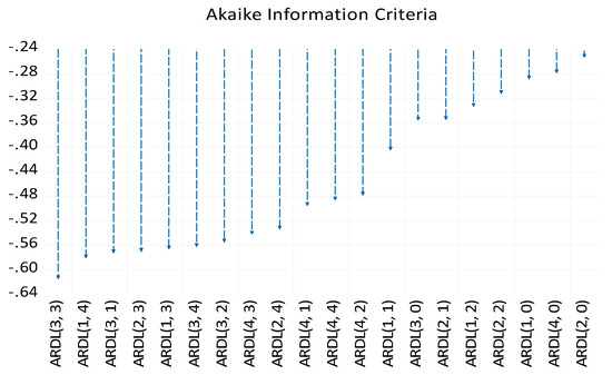
Figure 1.
Selection of the most closely fitted ARDL model, AIC criterion, lnU1, lnHE1 variables. Source: author’s processing, using EViews 12.
The main purpose for estimating an ARDL model is for it to be used as a basis for verifying the co-integration, the long-run relationship, between the analyzed variables. We used the ARDL long run form and bounds test to determine whether there was a long-run relationship between registered unemployment rate, lnU1, and the total number of individuals who have completed undergraduate university programs, lnHE1. The results are presented in Table 5. If the F-statistic value is higher than the upper limit (I(1), if the variable is stationary I(1) or I(0), if the variable is I(0)), estimated at a 5% significance, and if the absolute value of t-statistic is higher than the upper limit, estimated in absolute value, at a 5% significance threshold, then we can reject the null hypothesis, H0: there is no long-term co-integration between the two variables. In the present case, it is observed that the value of F-statistic is 1.105916 and therefore lower than the value of the upper limit, and the absolute value of t-statistic is −1.350886, lower than the absolute value of the upper limit, therefore we cannot reject the null hypothesis; between the two analyzed variables there is no long-term co-integration, only a short-run relationship. Thus, the construction of an error correction regression (ECM) to study the speed of system regulation in the situation of lack of co-integration between variables does not make sense. In terms of the short-run analysis, the increase in the total number of individuals who have completed undergraduate university programs caused a decrease in the registered unemployment rate in Romania during the analyzed period.
Table 5.
The results of the ARDL Long Form and Bounds Test, lnU1 and lnHE1.
Because the ARDL long form and bounds test shows the lack of co-integration between the variables lnU1 and lnHE1, there is no long-term equilibrium relationship between these two variables, but only a short-term relationship. The specification of the ARDL short-run model has the form:
where is the difference operator, p and q are the optimal lags for the dependent variable and for the explicative variable, and is the error term.
Since the estimation of the coefficients of the ARDL short-run model is done using the least squares method, we have to determine the optimal lag that we will use in specifying this model. To determine the optimal lag we use the Akaike information criterion (AIC), the Schwartz Bayesian criterion (SC), the Hannan-Quinn information criterion (HQ), the final prediction error (FPE), and the likelihood ratio test (LR). In Table 6 we present the results of finding the optimal lag for the dependent variable lnU1 and the explanatory variable lnHE1. We notice that three of the criteria, FPE, AIC and HQ, suggest that the optimal lag is 3, and two criteria, LR and SC, suggest that the optimal lag is 1. We will consider the optimal lag the one chosen by the most criteria; thus, the lag is 3.
Table 6.
Finding the optimal lag for lnU1, lnHE1.
The results of the estimation of Equation (3) for the variables lnU1 and lnHE1 are presented in Table 7. We notice that the registered unemployment rate is not significantly influenced by its own values with lag values 1, 2, and 3. The regression coefficients of these terms are negative, which would suggest an inverse link, but they are not significant.
Table 7.
Results of the ARDL short-run model lnU1, lnHE1.
According to the Breusch-Godfrey serial correlation test, there is no serial correlation in the ARDL short-run model, lnU1, lnHE1; the null hypothesis cannot be rejected, as we can see from Table 8.
Table 8.
The results of the Breusch-Godfrey serial correlation LM, lnU1, short-run, ARDL model.
We used the CUSUM and CUSUM of squares tests to check the stability of the ARDL short-run model. From Figure 2 and Figure 3 we can notice that the model is stable.
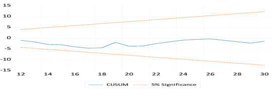
Figure 2.
CUSUM test, ARDL short-run, lnU1, lnHE1. Source: author’s processing, using EViews 12.
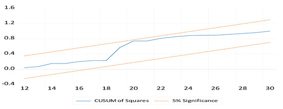
Figure 3.
CUSUM of squares test, ARDL short-run, lnU1, lnHE1. Source: author’s processing, using EViews 12.
The results of specifying the ARDL model for the variables total number of individuals who have completed undergraduate university programs and ILO unemployment rate, for the period 1996–2020, are presented in Table 9. The selection criterion used is again AIC, and as the maximum number of lags, we chose 4 for the endogenous variable and 4 lags for the independent variable.
Table 9.
ARDL model, dependent variable lnU2, independent variable lnHE2.
The error checking of this model was carried out using the Breusch-Godfrey serial correlation LM test. The results showed that null hypothesis, H0: there is no serial correlation up to lag 4, cannot be rejected, and so there is no serial correlation in the basic ARDL model, as described in Table 9. From Table 9 we can also notice that the selected model for this pair of variables is ARDL (3, 0); therefore, there are 3 lags for the dependent variable and 0 lags for the independent one. In Figure 4 we present the graphical visualization of the selection of the best-fitting ARDL model, based on the AIC selection criterion.
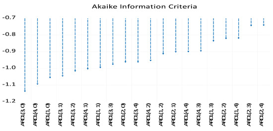
Figure 4.
Selection of the most closely fitted ARDL model, AIC criterion, lnU2, lnHE2. Source: author’s processing, using EViews 12.
As we previously pointed out, the specification of the ARDL model is used as a basis for checking the co-integration between the analyzed variables. The results of the long run form and bounds co-integration test are presented in Table 10. We can notice that both the F-statistic value and the t-statistic value (in absolute value) are less than both the lower limit and the upper limit at a significance threshold of 5%, which shows that there is no co-integration between the two analyzed variables. Therefore, we can conclude that there is no long-term equilibrium relationship between ILO unemployment rate and the total number of individuals who have completed undergraduate university programs. Moreover, for this time, the effect of the total number of individuals who have completed undergraduate university programs on the ILO unemployment rate is not significant, even in the short-term analysis.
Table 10.
The results of the ARDL Long Form and Bounds Test, lnU2 și lnHE2.
Next, we analyzed the optimal lag for the dependent variable lnU2 and the independent variable lnHE2. Four of the criteria, namely, LR, FPE, AIC and HQ, suggested that the optimal lag is 3. The results of estimating Equation (3) for the variables lnU2, lnHE2 are presented in Table 11. We notice that the ILO unemployment rate is not significantly influenced by its own values with lag 1, 2, and 3, or by the value of the total number of individuals who have completed undergraduate university programs, also with lag 1, 2 and 3.
Table 11.
Results of the ARDL short-run model lnU2, lnHE2.
The result of the serial correlation test is shown in Table 12. As we can notice, we cannot reject the null hypothesis, and, therefore, there is no serial correlation in the ARDL short-run model, lnU2, lnHE2.
Table 12.
The results of the Breusch-Godfrey serial correlation LM, lnU2, lnHE2.
We tested the stability of the ARDL short-run model with the CUSUM and CUSUM of squares tests, and the results are presented in Figure 5 and Figure 6. From the analysis of both figures, it follows that the model is stable.
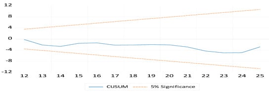
Figure 5.
CUSUM test, ARDL short-run, lnU2, lnHE2. Source: author’s processing, using EViews 12.
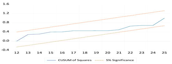
Figure 6.
CUSUM of squares tests, ARDL short-run, lnU2, lnHE2. Source: author’s processing, using EViews 12.
4. Conclusions
The aim of this paper was to investigate the potential long-run and/or short-run equilibrium relationships between higher education and unemployment for Romania. As a proxy for higher education, we used the total number of individuals who have completed university programs—first cycle (bachelor’s degree); statistical data describing the dynamic of this variable were collected from the Tempo-Online database of NIS for the periods 1991–2020 and 1996–2020. Unfortunately, statistical data on the number of graduates of master’s programs and Ph.D. programs are provided by the NIS only for the period 2014–2020, as annual data. Therefore, this information could not be used in the econometric analysis. This is a limitation of the study, but also a potential future research direction. As a proxy for unemployment, we used the registered unemployment rate, expressed as a percentage, for the period 1991–2020, and the ILO unemployment rate, also expressed as a percentage, for the period 1996–2020. As [51] underlined, the first study evaluating unemployment in Romania by the ILO standards was conducted in 1994. Thus, for the period 1991–1996, we do not have data on the ILO unemployment rate. As a research methodology, we used the ARDL model because it is a suitable approach for our datasets, ARDL being recommended by the literature for samples with a small number of observations and for variables with different degrees of stationarity. The results of the empirical analysis proved that there is no co-integration, either between the total number of individuals who have completed undergraduate university programs and the registered unemployment rate for the period 1991–2020, or between the total number of individuals who have completed undergraduate university programs and the ILO unemployment rate for the period 1996–2020. However, there is a significant short-run inverse relationship between the total number of individuals who have completed undergraduate university programs and the registered unemployment rate. In the short run, the total number of individuals who have completed undergraduate university programs causes a decrease in the registered unemployment rate, but has no significant effect on the ILO unemployment rate. The results of the study are similar to those obtained by [40], regarding the existence of a short-run inverse link between higher education and unemployment in Romania, but [40] also highlights a long-run relationship for the two variables. Our findings are in line with those obtained by [6] and [37], but only as to the short run. The results are, however, in opposition to the one obtained by [17], which highlights that the increase in the number of higher education graduates is one of the reasons that determine the increase in unemployment, both in the long-run and in the short-run, in Turkey during the period 1960–2007.
Although higher education improves the employment probability and shortens the unemployment duration of individuals in Romania [8,28,30], the results of this study showed that, at the macro-economic level, higher education and the unemployment rate are not co-integrated in the long run. In interpreting the obtained results, we must take into account the fact that, before the fall of the communist regime, the number of highly educated graduates was very low, and there was a shortage of highly qualified labor on the Romanian labor market. Additionally, the result emphasizes the importance, for a balanced and sustainable labor market, of correlating the number of individuals enrolled in higher education institutions with the needs of the labor market. If the investment in higher education will continue to be unbalanced, and without a correlation with the evolution of the labor market, we will witness a negative long-term effect of higher education on the unemployment rate. A non-sustainable increase in the number of highly educated graduates may become a cause of the increase of highly educated labor force unemployment and, of course, increased emigration of highly educated individuals to countries that offer increased integration with the labor market and a higher living standard. As [17] pointed out, if higher education causes a long-run increase in the unemployment rate, then governments should focus on new job creation and better job opportunities for highly educated individuals, instead of focusing only on increasing the number of highly educated graduates. The obtained results can be useful for policy makers and can contribute to the development of effective policies focused on higher education, which lead, in the long run, to sustainable economic growth. As [52] underlined, sustainable development of a society also means an optimal level of employment, which means a reduction of the unemployment rate to the value of its natural level.
As for future research directions, we will focus on investigating the causes that keep this substantial increase in the number of highly educated individuals from being reflected in the dynamics of the unemployment rate in the long run. We will analyze to what extent the education and training offered by the Romanian higher education institutions is consistent with the requirements of the labor market, with its dynamism and with the expectations of employers. We will also analyze the impact of digitalization on the labor market, on the demand and supply of labor force, and the role of Romanian universities in providing a labor force with digital skills, one which is flexible and able to adapt in the shortest possible time to the challenges brought by new technologies. Higher education is the engine of a modern knowledge economy; thus, these research directions are highly important for the sustainable development of society.
Author Contributions
All five authors contributed equally to this research work. All authors discussed the results and contributed to the final manuscript. All authors have read and agreed to the published version of the manuscript.
Funding
This research received no external funding.
Data Availability Statement
The data supporting reported results can be found at http://statistici.insse.ro:8077/tempo-online/#/pages/tables/insse-table.
Conflicts of Interest
The authors declare no conflict of interest.
References
- Denison, E. Why Growth Rates Differ? Postwar Experience in Nine Western Countries; The Brookings Institution: Washington, DC, USA, 1967; 494p. [Google Scholar]
- Mincer, J. Education and Unemployment. NBER Work. Pap. 1981, 3838, 1–34. [Google Scholar]
- Lucas, R.E. On the Mechanics of Economic Development. J. Monet. Econ. 1988, 22, 3–42. [Google Scholar] [CrossRef]
- Barro, R.J. Economic Growth in a Cross-Section of Countries. Q. J. Econ. 1991, 106, 407–443. [Google Scholar] [CrossRef]
- Dickens, W.T.; Sawhill, I.; Tebbs, J. The Effects of Investing in Early Education on Economic Growth. Policy Brief, 153, The Brookings Institutions. 2006. Available online: https://www.brookings.edu/wp-content/uploads/2016/07/200604dickenssawhill.pdf (accessed on 21 November 2022).
- Núñez, I.; Livanos, I. Higher Education and Unemployment in Europe: An Analysis of the Academic Subject and National Effects. High. Educ. 2010, 59, 475–487. [Google Scholar] [CrossRef]
- Maneejuk, P.; Yamaka, W. The Impact of Higher Education on Economic Growth in ASEAN-5 Countries. Susteinability 2021, 13, 520. [Google Scholar] [CrossRef]
- Dănăcică, D.E. Employment and Unemployment of Highly Educated Labor Force in Romania; Academica Brâncuși Publishing House: Târgu-Jiu, Romania, 2022; pp. 25–75. [Google Scholar]
- Stevens, P.; Weale, M. Education and Economic Growth. NIESR Working Paper. 2003. Available online: http://cee.lse.ac.uk/conference_papers/28_11_2003/martin_weale.pdf (accessed on 15 November 2022).
- Lazic, Z.; Ðordevic, A.; Gazizulina, A. Improvement of Quality of Higher Education Institutions as a Basis for Improvement of Quality of Life. Sustainability 2021, 13, 4149. [Google Scholar] [CrossRef]
- Ram, R. Educational Expansion and Schooling Inequality: International Evidence and Some Implications. Rev. Econ. Stat. 1990, 72, 266–274. [Google Scholar] [CrossRef]
- McKenna, C.J. Education and the Distribution of Unemployment. Eur. J. Polit. Econ. 1996, 12, 113–132. [Google Scholar] [CrossRef]
- Domadenik, P.; Pastore, F. The Impact of Education and Training Systems on the Labour Market Participation of Young People in CEE Economies. A Comparison of Poland and Slovenia. GDN Research Report. 2004. Available online: https://www.cerge-ei.cz/pdf/gdn/rrc/RRCIII_50_paper_01.pdf (accessed on 21 November 2022).
- Niepel, V. The Importance of Cognitive and Social Skills for the Duration of Unemployment; ZEW Discussion Papers No. 10-104; Zentrum für Europäische Wirtschaftsforschung (ZEW): Mannheim, Germany, 2010. [Google Scholar]
- Podrecca, E.; Carmeci, G. Does Education Cause Economic Growth? DiSES Working Papers 96B; University of Trieste: Trieste, Italy, 2002. [Google Scholar]
- Gregorio, J.D. Economic Growth in Chile: Evidence, Sources and Prospects; Working Papers of Central Bank of Chile 298; Central Bank of Chile: Santiago, Chile, 2004. [Google Scholar]
- Erdem, E.; Tugcu, C.T. Higher Education and Unemployment: A Cointegration and Causality Analysis of the Case of Turkey. Eur. J. Educ. 2012, 47, 299–309. [Google Scholar] [CrossRef]
- Pillay, P. Higher Education and Economic Development. Literature Review; Centre for Higher Education Transformation: Cape Town, South Africa, 2011; pp. 1–7. Available online: https://www.borbolycsaba.ro/wp-content/uploads/2013/09/Higher-Education-and-Economic-Development-Literature-Review.pdf (accessed on 2 February 2023).
- Wolf, A. Does Education Matter? Myths about Education and Economic Growth; Penguin Publishing Group: London, UK, 2002; p. 3. [Google Scholar]
- UNESCO. Available online: https://www.unesco.org/en/higher-education (accessed on 2 February 2023).
- Bai, L. Graduate Unemployment: Dilemmas and Challenges in China’s Move to Mass Higher Education. China Q. 2006, 185, 128–144. [Google Scholar] [CrossRef]
- Li, S.; Whalley, J.; Xing, C. China’s Higher Education Expansion and Unemployment of College Graduates. China Econ. Rev. 2014, 30, 567–582. [Google Scholar] [CrossRef]
- Lubyova, M.; van Ours, J. Unemployment Dynamics and the Restructuring of the Slovak Unemployment Benefit System. Eur. Econ. Rev. 1997, 41, 925–934. [Google Scholar] [CrossRef]
- D’Agostino, A.; Mealli, F. Modeling Short Unemployment in Europe; ISER Working Paper; Institute for Social & Economic Research: Essex, UK, 2000. [Google Scholar]
- Grogan, L.; van den Berg, J. Determinants of Unemployment in Russia. J. Popul. Econ. 2001, 14, 549–568. [Google Scholar] [CrossRef]
- Farber, H.S. Job Loss in the United States, 1981 to 2001. In Accounting for Worker Well-Being, Research in Labor Economics; Polachek, S.W., Ed.; Emerald Group Publishing Limited: Bingley, UK, 2004; pp. 69–117. [Google Scholar]
- Ollikainen, V. Gender Differences in Unemployment in Finland. Doctoral Thesis, University of Jyvaskyla, Jyväskylän yliopisto, Finland, 2006. Chapter 4. pp. 82–110. Available online: https://jyx.jyu.fi/bitstream/handle/123456789/13191/9513925609.pdf (accessed on 24 November 2022).
- Kavkler, A.; Danacica, D.E.; Babucea, A.G.; Bicanic, I.; Bohm, B.; Tevdovski, D.; Tosevska, K.; Borsic, D. Cox Regression Models for Unemployment Duration in Romania, Austria, Slovenia, Croatia, and Macedonia. Rom. J. Econ. 2009, 6, 81–104. [Google Scholar]
- Dănăcică, D.E. The Impact of Factors Influencing Unemployment Duration and Exit Destinations of Higher Educated People in Romania and Hungary. Stud. UBB Oeconomica 2012, 57, 3–26. [Google Scholar]
- Dănăcică, D.E. The Effect of Factors Influencing Unemployment Duration and (Re)employment Probability (Cercetări Privind Impactul Factorilor ce Influenţează Durata Şomajului şi Probabilitatea (Re)angajării în România); Expert Publishing House: Bucharest, Romania, 2013; pp. 44–84. [Google Scholar]
- Foley, M.C. Determinants of Unemployment Duration in Russia; Center Discussion Paper No. 770; Yale University: New Haven, CT, USA, 1997; Available online: https://core.ac.uk/download/pdf/7056835.pdf (accessed on 23 November 2022).
- Kettunen, J. Education and Unemployment Duration. Econ. Educ. Rev. 1997, 2, 163–170. [Google Scholar] [CrossRef]
- Wolbers, M.H.J. The Effect of Education on Mobility between Employment and Unemployment in Netherlands. Eur. Sociol. Rev. 2000, 16, 185–200. [Google Scholar] [CrossRef]
- Woodley, A.; Brennan, J. Higher Education and Graduate Employment in the United Kingdom. Eur. J. Educ. 2000, 35, 239–249. [Google Scholar] [CrossRef]
- Schomburg, H. Higher Education and Graduate Employment in Germany. Eur. J. Educ. 2000, 35, 189–200. [Google Scholar] [CrossRef]
- Plümper, T.; Schneider, C.J. Too Much to Die, too Little to Live: Unemployment, Higher Education Policies and University Budgets in Germany. J. Eur. Public Policy 2007, 14, 631–653. [Google Scholar] [CrossRef]
- Qazi, W.; Ali Raza, S.; Sharif, A. Higher Education Development and Unemployment in Pakistan: Evidence from Structural Break Testing. Glob. Bus. Rev. 2017, 18, 1089–1110. [Google Scholar] [CrossRef]
- Florea, S.; Oprean, C. Towards an Integrated Project: Higher Education and Graduate Employment in Romania. Manag. Sustain. Dev. 2010, 2, 78–85. [Google Scholar]
- Naghi, D.I. Young Graduates Are Looking for Jobs! Between Education and the Labor Market. Eur. J. Soc. Sci. 2014, 1, 86–90. [Google Scholar] [CrossRef]
- Mirică, A. Higher Education—A Solution to Unemployment? Case Study: Romania. Rev. Rom. Stat. 2014, 3, 63–75. [Google Scholar]
- Mroz, T.A.; Savage, T.H. The Long-Term Effects of Youth Unemployment. J. Hum. Resour. 2006, 41, 259–293. [Google Scholar] [CrossRef]
- Bell, D.N.F.; Blanchflower, D.G. Young People and the Great Recession. IZA DP No. 5674. 2011. Available online: https://www.econstor.eu/bitstream/10419/52080/1/666568758.pdf. (accessed on 19 November 2022).
- Bartlett, W.; Uvalić, M.; Durazzi, N.; Monastiriotis, V.; Sene, T. From University to Employment: Higher Education Provision and Labour Market Needs in the Western Balkans; European Comission: Brussels, Belgium, 2006; Available online: http://www.lse.ac.uk/business-and-consultancy/consulting/assets/documents/From-University-to-Employment.pdf (accessed on 18 November 2022).
- Gagea, M. Identificarea transformărilor necesare staționarizării unei serii de timp. Ann. Alexandru Ioan Cuza Univ. Iași 2005, 50, 432–438. [Google Scholar]
- Gujarati, D.N.; Porter, D.C. Basics Econometrics, 5th ed.; McGraw-Hill Companies, Inc.: New York, NY, USA, 2009; pp. 737–773. [Google Scholar]
- Granger, C.W.J.; Newbold, P. Spurious Regressions in Econometrics. J. Econom. 1974, 2, 111–120. [Google Scholar] [CrossRef]
- Cheng, B.S. An Investigation of Cointegration and Causality Between Fertility and Female Labour Force Participation. Appl. Econ. Lett. 1996, 3, 29–32. [Google Scholar] [CrossRef]
- Pesaran, M.H.; Shin, Y. An autoregressive distributed lag modelling approach to cointegration analysis. In Econometrics and Economic Theory in the 20th Century: The Ragnar Frisch Centennial Symposium 1998; Strom, S., Ed.; Cambridge University Press: Cambridge, UK, 1999; Chapter 11, Part V; pp. 371–413. [Google Scholar]
- Pesaran, M.H.; Shin, Y.; Smith, R.J. Bounds Testing Approaches to the Analysis of Level Relationships. J. Appl. Econ. 2001, 16, 289–326. [Google Scholar] [CrossRef]
- Shrestha, M.B.; Bhatta, G.R. Selecting appropriate methodological framework for time series data analysis. J. Financ. Data Sci. 2018, 4, 71–89. [Google Scholar] [CrossRef]
- Bădulescu, A. Unemployment in Romania. A Retrospective Study. Theor. Appl. Econ. 2006, 2, 71–76. [Google Scholar]
- Zaman, G. Dezvoltarea Durabilă, Imperativ Pentru Prezentul şi Viitorul României. In Dezvoltarea Durabilă in Secolul XXI, Revista 22. 2006. Available online: https://revista22.ro/supliment/este-posibila-o-dezvoltare-durabila-in-romania (accessed on 2 February 2023).


Disclaimer/Publisher’s Note: The statements, opinions and data contained in all publications are solely those of the individual author(s) and contributor(s) and not of MDPI and/or the editor(s). MDPI and/or the editor(s) disclaim responsibility for any injury to people or property resulting from any ideas, methods, instructions or products referred to in the content. |
© 2023 by the authors. Licensee MDPI, Basel, Switzerland. This article is an open access article distributed under the terms and conditions of the Creative Commons Attribution (CC BY) license (https://creativecommons.org/licenses/by/4.0/).