Environmental Condition Boundary Design for Direct-Drive Permanent Magnet (DDPM) Wind Generators by Using Extreme Joint Probability Distribution

Abstract

In future engineering applications, it is important for a direct-drive permanent magnet (DDPM) wind generator to be designed with optimized environmental condition boundary. This paper presents a novel extreme joint probability distribution method of boundary design to formulate the evaluation model and correlation between component design and environmental conditions. With this method, the joint probability distributions of multidimensional parameters for typical wind resource areas in China are studied. A 3.3-MW DDPM wind generator is involved in the case study to validate the superiority of the method. Furthermore, to improve the generalizability of the method, some typical wind resource data platforms are calibrated regarding the measured data. It is shown that the ERA5 dataset can be used as a supplement to enhance the representativeness of the measured data for the joint probability distributions. Therefore, the proposed method can be potentially used to optimize the system design of future DDPM wind generators.

1. Introduction

Recent years have seen growing focus on direct-drive permanent magnet (DDPM) wind generators owing to their higher reliability and better performance. However, with increasing scale of wind generators and complexity of operating environmental conditions, it is of great importance to study and reveal the relationship between the environmental condition and generator designing boundary.

Some studies propose probability methods for wind turbine design optimization. For example, a probabilistic integrated multidisciplinary approach is used for designing optimization of MW-level wind turbines considering the stochastic variability of the mean wind speed [1]. With this approach, the wind speed frequency distribution can be involved in blade dynamics design, so that the levelized cost of energy (LCOE) is about 12.7% lower than when using traditional deterministic designing methods. Some other studies aim to model a more complete environmental joint distribution for probabilistic analysis of offshore structures or renewable energy modules with reduced design conservatism and more accurate distribution [2,3]. In [4], a probabilistic framework is designed to assess the structural reliability of wind turbines in fatigue load, with validation in flat terrain, which shows that the uncertainty in the wind climate parameters accounts for 10~30% of the total uncertainty in the structural reliability.

However, most of the above studies focus on the joint probability analysis or uncertain influence of environmental conditions on the limit or fatigue load of structural components [5,6], whereas for the electrical components of a wind turbine, especially for wind generators, there should be more applicable optimization methods that use available data [7,8,9]. More specifically, most traditional methods regard the environmental conditions as individual variables, which may lead to conservative design results. Actually, from the view of engineering applications, the effects of wind, temperature, altitude, and operation period on the wind generator design are coupled, so the mutual coupling relationship among these environmental variables should be considered in generator design. In addition, the situation wherein multiple environmental parameters reach the maximum values simultaneously during the recurrence period should be considered as well. Consequently, using current generator design methods without considering the above issues may lead to the fact that the environmental design boundaries exceed the operating environmental conditions, so there may exist lower power density of generator as well as more waste of materials. In conclusion, it is a vital issue to formulate the relationship between the design boundaries of the wind generator and joint probability of environmental conditions. That is, the environmental design boundaries for wind generator design can be further optimized to ensure the reliability of system operation while also keeping high power density and material utilization. This is one of the issues to be addressed in this study.

Another issue is related to the evaluation method of wind generator design. Due to the increasing complexity of large-scale wind generators, the way to evaluate the effects of varying design parameters on the economy of generators is a challenging topic. Currently, most studies use the LCOE for comprehensive evaluation of system economy. For example, NREL formulates a wind generator model to predict the cost with varying wind turbine capacities, and also provides the tools with which to evaluate the effects of the difference between capacity and configuration on the total cost of energy [10]. In [11], a wind farm with 6–20-MW wind turbines is analyzed by using the LCOE to evaluate the coupled effects of wind farm scale and system cost on offshore wind power development. Some other studies use LCOE and wind statistical methods to minimize the system cost and provide design principles of determining the optimal wind power curve and rated wind speed curve [12].

However, current LCOE-based evaluation methods for wind generator design mainly focus on evaluating the economic effect of generator capacity and system configuration on wind farm construction, whereas less analysis has been done on the influence of the varying generator designing elements on the whole wind turbine performance, and thus no further optimization can be performed. That is, it is still necessary to optimize the wind generator design boundaries by blending the LCOE evaluation with multiple scheme selection, so as to formulate a straightforward and feasible scheme for engineering applications.

To address the above issues, this paper presents an environmental condition boundary design method for DDPM generators (DDPMGs) by using extreme joint probability distribution.

The key contributions of this work can be summarized as follows.

(1)

By considering the unique characteristics of MW-level DDMPG design and operation, we analyze the key parameters of environmental conditions that affect the generator designing boundaries. These key parameters involve the wind speed, environmental temperatures, altitude, and wind duration period. The correlation mechanisms of these parameters are shown by using the upcoming joint probability distribution method. The coupled relationship between the DDPMG designing boundaries and environmental conditions can thus be revealed.

(2)

To select the optimal DDPMG designing scheme and perform LCOE evaluation, an extreme joint probability distribution method is designed for the environmental conditions. The 3.3.3-MW Goldwind DDPMG and datasets from five typical wind farms of China are used for experimental validation, demonstrating the joint mechanism of the key parameters and effectiveness of the proposed method on boundary optimization.

The rest of the paper is organized as follows. The key parameters of environmental conditions are analyzed in Section 2. The proposed environmental condition boundary design method for DDPM wind generators by using extreme joint probability distribution is proposed in Section 3. Case studies in multiple Chinese regions are performed in Section 4. The extended wind resource data simulation platforms are analyzed to discuss the representativeness of the datasets in Section 5. Finally, the conclusions and discussions are provided in Section 6.

2. Analysis on the Key Parameters of Environmental Conditions

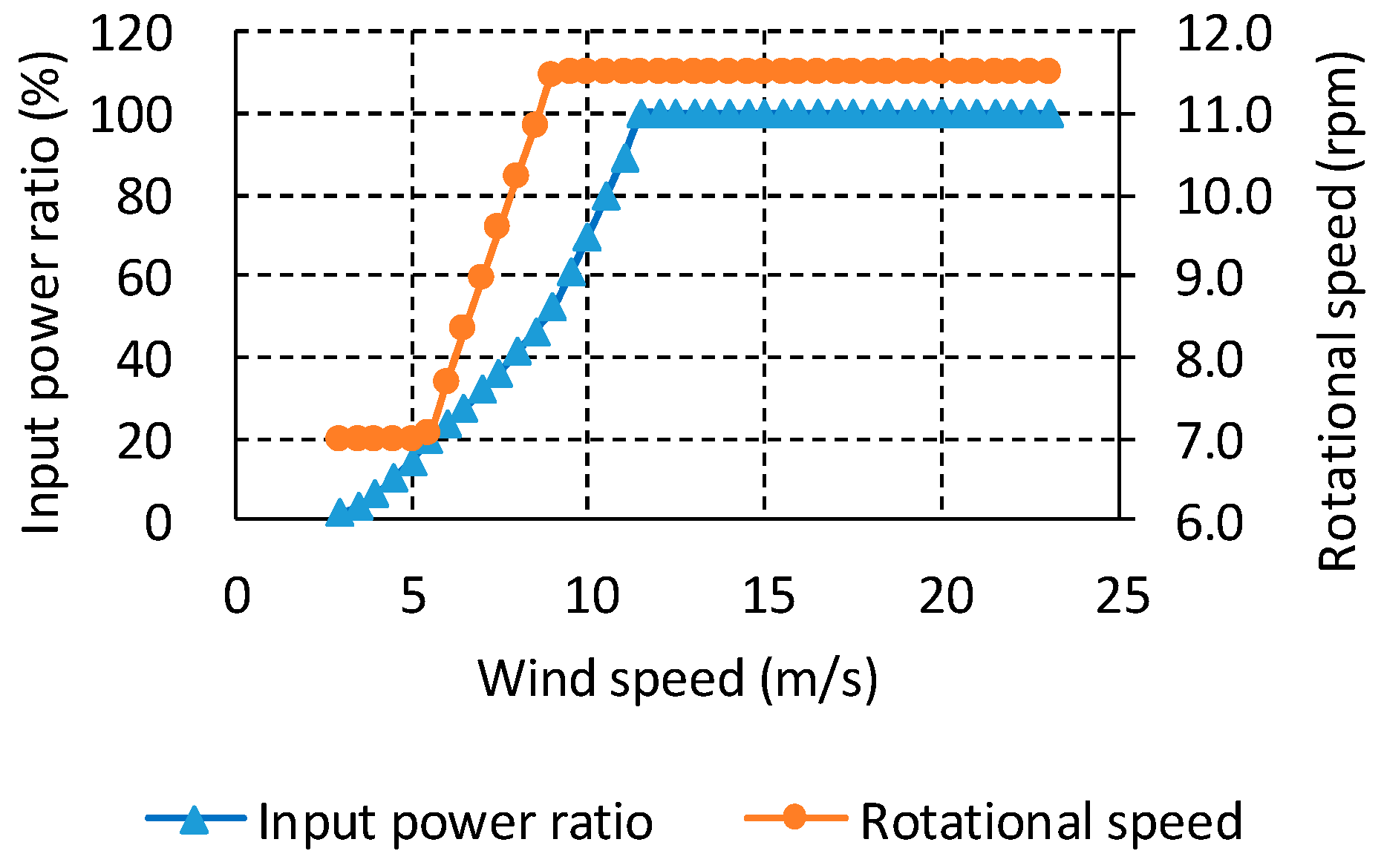
2.1. Effects of Wind Speed on Operating Characteristics of DDPMG

For the DDPMGs, the operating characteristics are directly related to the wind speed. Figure 1 shows the input power ratio curve and rotational speed curve versus wind speed. Note that the generator rotational speed of DDPMG is consistent with the rotor speed, so we get the generator efficiency curve with considering the electromagnetic losses, as shown in Figure 2. From Figure 1 and Figure 2 we can see that the initially increasing wind speed enables the rapid rise of output power ratio and efficiency, and the peak value is located on the point where the output power is approximately 20% of the rated power. Then, further increasing output power leads to higher generator copper loss, so that the efficiency becomes a bit lower. In conclusion, the operation characteristics are closely related to the wind speed.

2.2. Effects of Ambient Temperature and Altitude on Operating Characteristics of DDPMG

For designing a DDPMG, the maximum winding temperature is directly related to the environmental conditions, such as the ambient temperature and altitude, which have direct effects on the safe operation of the generator. This is because the generator produces heat during electricity production, whereas for different ambient temperatures and altitudes, the generator cooling system design should be correspondingly adjusted to ensure that the winding temperature can be kept within the allowable material temperature range. Generally, the generator cooling system should be designed to ensure that the generator can operate at the full power continuously in the whole operating ambient temperature range without exceeding the maximum allowable working temperature of the material. Engineering applications have shown that for the DDPMGs, the winding is the dominating source of heat, accounting for approximately 80% of the total heat loss. Then, with IEC standards [13,14], as well as the above analysis on DDPMGs, we provide the unique evaluation principle for the winding temperature rise versus ambient temperature and altitude, so we get the maximum winding temperature in terms of different ambient temperature boundary conditions as

$$T_H=\Delta T_H+T_{eH}=\Delta T_0\frac{235+T_{eH}}{235+T_{e0}}\left(1+\frac{H}{10000}\right)+T_{eH},$$

(1)

where $T_H$, $\Delta T_H$, and $T_{eH}$ are the maximum winding temperature (°C), maximum winding temperature rise (K), and maximum ambient temperature (°C), in some certain operating environment conditions, respectively. $\Delta T_0$ is the allowable maximum winding temperature rise in the condition of 0 m altitude and corresponding maximum ambient temperature (K), $T_{e0}$ is the maximum ambient temperature at 0 m altitude (°C), and $H$ denotes the actual altitude under some certain operating environment condition (m).

According to (1), when the maximum winding temperature reaches the upper allowable operating temperature, the corresponding ambient conditions, i.e., $T_{e{H}_{MAWT}}$ and $H_{MAWT}$ in (2), are called the boundaries of environmental conditions for safe operation of a generator, described as

$$T_{H_{MAWT}}=\Delta T_H+T_{e{H}_{MAWT}}=\Delta T_0\frac{235+T_{e{H}_{MAWT}}}{235+T_{e0}}\left(1+\frac{H_{MAWT}}{10000}\right)+T_{e{H}_{MAWT}}.$$

(2)

2.3. Effects of Wind Duration Period on Operating Characteristics of DDPMG

According to Section 2.1 and Section 2.2, the operating process of the DDPMG is transient because the random change of natural wind, although the safe operation also relies on the maximum allowable temperature of material. Therefore, for the material used in the generator, the heat capacity is related to the duration period of each part to reach the maximum allowable operating temperature. The heat capacity of the material is defined as

$$C_t=C_i{\rho }_i{V}_i,$$

(3)

where $C_i$ is the heat capacity (J/kg·K⁻¹) and ${\rho }_i$ and $V_i$ are the material density (kg/m³) and volume (m³), respectively.

Clearly, a larger heat capacity needs a longer time to reach the maximum allowable operating temperature. For MW-level large-scale DDPMGs, the heat capacity is relatively large, so it takes a longer time for the DDPMG to transfer from the cold state to the heat stable state, compared to double-fed induction generators (DFIGs). Experiments show that it may take about 2~3 h for a 3.3-MW DDPMG to reach the stable state of heat after start-up, as shown in Figure 3.

From the above analysis on the key parameters of environmental conditions provided by Section 2.1, Section 2.2 and Section 2.3, we can get the following basic conclusions for DDPGM boundary design.

(a)

Some key environmental conditions may have direct influence on the DDPMG operating speed, input power, operating efficiency, maximum winding temperature for safe operation, and the period of reaching stable temperature. These conditions include the wind speed, ambient temperature, altitude, and wind duration period.

(b)

When the wind speed varies between 3 m/s and 25 m/s, the generator rotational speed, input, and output power, as well as the operating efficiency will be located at different characteristic operating points. The component temperature can reach the maximum steady-state temperature only when the wind speed continues for a certain period of time in the rated power range.

(c)

According to Equations (1) and (2), to ensure that the operating temperature does not exceed the maximum allowable operating temperature of the material, although the generator can operate for a long time under different combination of ambient temperature and altitude, the ambient temperature corresponding to the altitude of 1000 m can be used as the baseline of the ambient temperature boundary conditions for safe operation.

For the precise design process of DDPMG, comprehensive analysis and optimization should be made with considering the above effects of ambient conditions. More specifically, an extreme joint probability distribution method of boundary design is to be proposed as follows to formulate the evaluation model and analysis process of the correlation between component design and environmental conditions.

3. Extreme Joint Probability Distribution Method of Boundary Design

As stated before, the environmental conditions are the key design boundary conditions for DDPMG design. Compared to traditional deterministic design methods, which may lead to conservativeness and higher cost, the proposed extreme joint probability distribution method ensures precise designing boundaries with higher material utilization ratio. First, the LCOE evaluation model is provided as follows.

3.1. Cost Model Based on LCOE

The cost model describes the relationship between the generator design and economy. Adjusting the design scheme leads to varying system cost and performance. Thus, the LCOE is usually adopted for evaluation [10]. It can be described as

$$LCOE=\frac{(CAPEX-T_{de}\times R_{dis}-V\times R_{dis})+OPEX\times R_{dis}}{AEP\times R_{dis}},$$

(4)

where $CAPEX$ is the capital expenditure, $AEP$ is the annual energy production, $T_{de}$ is the discount against tax, $R_{dis}$ is the discount rate, $V$ is the salvage value, and $OPEX$ is the operating expenditure.

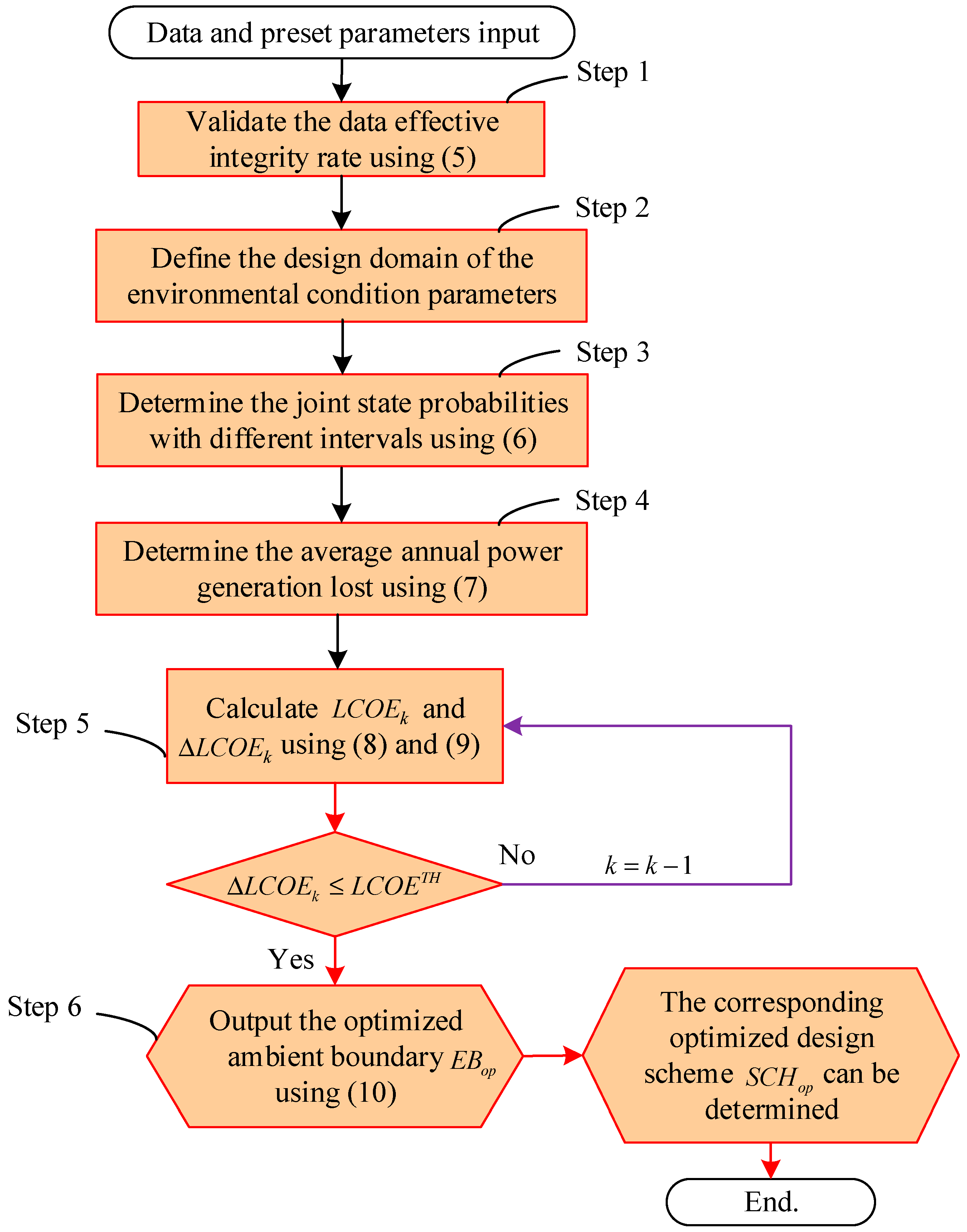
3.2. Evaluation Method and Process of the Proposed Method

The basic implementation steps of the proposed joint probability distribution statistical method based on environmental conditions are given as follows.

• Step 1: Validate the datasets of environmental condition parameters.

The environmental condition parameters used for analysis are N years of historical data obtained from the measurements of wind towers and wind turbines. The wind measuring towers are set in the target wind field to analyze the actual situation of the wind energy resources. Considering the efficiency of data statistics, the original data are first converted into average data with the interval of 10 min. Then, to ensure the validity of the data, the rationality and integrity of the data are checked. Reasonableness verification can be conducted through the reasonable range test of main parameter values (including wind speed, wind direction, and temperature) and the correlation test of average wind speed difference at different heights, as well as the average variation trend of the key parameter values per unit hour. Integrity verification includes quantitative and time sequence check, to ensure that the integrity of data sources included in statistics is larger than 90%. That is, the data effective integrity rate $VID$ should be

$$VID=\frac{MD-LD-AD}{MD}\ge 90\%,$$

(5)

where $MD$, $LD$, and $AD$ denote the measurement data, missing data, and abnormal data, respectively. Note that all wind speed values should be standardized by using the wind speed value at the height where the dominating number of wind turbine hubs are located.

• Step 2: Define the design domain of the environmental condition parameters.

We take the ambient temperature and wind speed as examples to define the design domain.

The parameter range of ambient temperature is expressed as [$D_{En}^L$, $D_{En}^U$], where $D_{En}^L$ and $D_{En}^U$ denote the lower limit and upper limit, respectively. Similarly, the parameter range of wind speed can be expressed as [$D_v^L$, $D_v^U$], where $D_v^L$ and $D_v^U$ denote the lower limit and upper limit, respectively.

The parameter range of ambient temperature is divided into $m$ ambient temperature subintervals, denoted as [$D_{En}^L+i\times {\delta }_{En}$, $D_{En}^L+(i+1)\times {\delta }_{En}$], where $i\in [0,m-1]$; ${\delta }_{En}$ is the temperature interval, and $D_{En}^L+i\times {\delta }_{En}$ and $D_{En}^L+(i+1)\times {\delta }_{En}$ are the lower and upper limits of this subinterval, respectively. Similarly, the parameter range of wind speed is divided into $n$ wind speed subintervals, denoted as [$D_v^L+j\times {\delta }_v$,$D_v^L+(j+1)\times {\delta }_v$], where $j\in [0,n-1]$, ${\delta }_v$ is the wind speed interval, $D_v^L+j\times {\delta }_v$ and $D_v^L+(j+1)\times {\delta }_v$ are the lower limit and upper limit of this subinterval, respectively.

• Step 3: Determine the joint state probabilities with different intervals.

The ith subinterval of ambient temperature and the jth subinterval of wind speed form an interval combination. Thus, the $m$ ambient temperature subintervals and $n$ wind speed subintervals constitute multiple combinations. Clearly, the generator has different joint state probabilities in different interval combinations. Herein, the joint probability is used to identify the cumulative duration proportion of the target wind generator under different interval combinations, and can be described as

$$P_{En\_v}^{(i,j)}=\frac{{\displaystyle {\sum }_1^{k1}{t}_1^{En\_v}}+{\displaystyle {\sum }_1^{k2}{t}_2^{En\_v}}}{{\tau }_1\cdot {\displaystyle {\sum }_1^{k1}(t_1^r-t_1^l-t_1^s)+{\tau }_2\cdot {\displaystyle {\sum }_2^{k1}(t_2^r-t_2^l-t_2^s)}}},$$

(6)

where $P_{En\_v}^{(i,j)}$ is the joint probability, $k_1$ and $k_2$ are the numbers of the generators and wind measuring towers in the target wind farm, respectively, ${\tau }_1$ and ${\tau }_2$ are the designing correction errors of the generators and wind measuring towers, taken from the range of [1, 5] and [1, 3], respectively, $t_1^r$ and $t_2^r$ are the start time and stop time of the generators and wind measuring towers, respectively, $t_1^l$ and $t_2^l$ are the duration time of missing data for the generators and wind measuring towers, respectively, and $t_1^s$ and $t_2^s$ are the duration time of abnormal data for the generators and wind measuring towers, respectively. $t_1^{En\_v}$ and $t_2^{En\_v}$ are the total operation time of the generators and wind measuring towers, under the interval combination composed of the ith subinterval of ambient temperature and the jth subinterval of wind speed.

Note that the total operation time refers to the wind duration period which equals to the time interval that the components reach the stable states of heat. According to the operation characteristics of electrical components in wind turbines, three kinds of duration (30 min, 2 h and 4 h) are defined. For example, the temperature rise stability time of IGBT in the converter is 30 min; the thermal stability time of grid-side reactor, current-sharing reactor, du/dt and fast melting time are all set as 2 h; the thermal stability time of the capacitor and bus system is 4h; the thermal stability time of the winding and magnetic steel of the DDPMG is about 2 h to 3 h. Thus, various target components correspond to different wind duration periods.

• Step 4: Determine the average annual power generation loss with different intervals.

When the actual operating environment conditions of the unit exceed the environmental conditions corresponding to the maximum allowable operating temperature of components, the unit will implement the capacity limit operation strategy for safety protection, which leads to the annual average power generation loss. On the other hand, when the environmental conditions of turbine design are reduced, the combined effect of reducing the component design cost and loss of power generation will result in the decrease of LCOE. This inspires us to narrow the range of environmental conditions.

The annual average power generation loss is defined as

$$AE{P}_{loss}^i=8760\times P_r\times P_{En\_v}^{(i,\gamma )}\times {\eta }_d\times {\eta }_a,$$

(7)

where $P_r$ is the rated capacity of the target wind turbine, ${\eta }_d$ is the operational loss ratio with limited capacity usually set between 5~10%, and ${\eta }_a$ is the availability of wind turbine. For a given wind farm, if the target wind generator is under the wind speed of the full power operation, the heating components of the generator are kept under the most severe environmental conditions. In this case, the subinterval of wind speed is fixed as $\gamma$, so the subinterval of ambient temperature can be selected among the $m-1$ possible subintervals, and the joint possibility under the wind speed of the full power operation can thus be denoted as $P_{En\_v}^{(i,\gamma )}$. Then, by using (7), the annual average power generation loss under full power operation but different ambient temperatures can be derived.

• Step 5: LCOE-based scheme selection and ambient condition boundary optimization.

By defining $E{B}_k$ as the upper bound of the $k$th ambient subinterval, we get the corresponding design scheme denoted as $SC{H}_k$. With (4) and (7), the LCOE is derived using $SC{H}_k$, as

$$LCO{E}_k=\frac{(CAPE{X}_k-TDE\times R_{dis}-V\times R_{dis})+OPEX\times R_{dis}}{(AE{P}_k-AE{P}_{loss}^k)\times R_{dis}},$$

(8)

where $CAPE{X}_k$ and $AE{P}_k$ are the capital expenditure and annual energy production using $SC{H}_k$, respectively. $AE{P}_{loss}^k$ can be computed by using (7).

Similarly, the design scheme $SC{H}_{k-1}$ can be formulated to compute the $LCO{E}_{k-1}$ for the $k-1$th ambient subinterval. Then, we have the LCOE difference between the two adjacent ambient subintervals with $SC{H}_k$ and $SC{H}_{k-1}$, respectively, as

$$\Delta LCO{E}_k=\frac{\left|LCO{E}_{k-1}-LCO{E}_k\right|}{LCO{E}_k}\times 100\%.$$

(9)

With (9), a calculation loop starts from $k=m-1$ when the subinterval corresponds to $[D_{En}^L+k\times {\delta }_{En}, D_{En}^L+(k+1)\times {\delta }_{En}]$, with the corresponding LCOE difference as $\Delta LCO{E}_k$. If $\Delta LCO{E}_k$ is larger than the preset threshold $\Delta LCO{E}^{TH}$, we set $k=m-2$ and compare $\Delta LCO{E}_{k-1}$ to $\Delta LCO{E}^{TH}$. The loop will not stop until the LCOE difference $\Delta LCO{E}_{\beta }$ ensures that $\Delta LCO{E}_{\beta }\le \Delta LCO{E}^{TH}$. Then the optimized available ambient boundary is updated as $[D_{En}^L, D_{En}^L+\beta \times {\delta }_{En}]$.

• Step 6: Output the optimized ambient boundary $E{B}_{op}$ and corresponding design scheme $SC{H}_{op}$.

With the computation results of Step 5, we get the upper bound of the optimized ambient boundary $[D_{En}^L, D_{En}^L+\beta \times {\delta }_{En}]$ as

$$E{B}_{op}=D_{En}^L+\beta \times {\delta }_{En}.$$

(10)

The optimized design scheme denoted by $SC{H}_{op}$ can thus be determined as well using the computed $E{B}_{op}$ and corresponding input variables of generator design.

In conclusion, the overall steps of the above joint probability distribution statistical method based on environmental conditions can be shown in Figure 4.

4. Case Studies of Typical Regions in China

4.1. Analysis of Environmental Conditions in Typical Land Areas of China

The data of 1550 wind towers and 9543 wind turbines in North China, Central China, East China, Northwest and Northeast China are used. Data validation indicates that 606 wind towers and 5414 wind turbines are available for the upcoming case studies. The wind tower distribution of the multiple target provinces in China is shown in Figure 5.

Then, the parameter designing regions are defined. The parameter range of wind speed is set as [9 m/s, 12 m/s], with the interval 0.5 m/s, the parameter range of ambient temperature is set as [25 °C, 40 °C], with the interval 1 °C, and the parameter range of altitude is set as [0 m, 2500 m], with the interval 250 m when the altitude is above 1000 m. The wind duration periods are taken as 30 min, 2 h, and 4 h, respectively.

With the above regions, multiple interval combinations are derived, including the relational matrix of ambient temperature versus wind speed with varying altitude intervals, the relational matrix of ambient temperature versus altitude with varying wind speed intervals, the relational matrix of ambient temperature versus wind speed with varying duration periods, etc. Consequently, the joint state probabilities with different intervals are calculated by using Equation (6).

For five typical regions in North China, Central China, East China, and Northwest and Northeast China, the joint probabilities are plotted. Figure 6 shows the joint probabilities of ambient temperature versus altitude, with the 2-h wind duration period and wind speed higher than 10 m/s. Figure 7 shows the joint probabilities of ambient temperature versus wind speed, with the 2-h wind duration period and altitude range of [0 m, 1000 m].

It can be concluded from Figure 6 that among the five typical regions in China, the North China region has the widest temperature and altitude ranges of distribution. The maximum joint probability is 1.39%, which appears in the altitude range of [1250 m, 1500 m] with the ambient temperature larger than 25 °C. The maximum joint probability of temperature occurs in [1250 m, 1500 m] as well, with the ambient temperature higher than 37 °C, which means that there is little probability that the wind speed is greater than 10 m/s and the ambient temperature is greater than or equal to 37 °C for 2 h within this altitude range. For the other four regions (Central China, East China, Northwest and Northeast China), we can find the following.

(a)

The northwest region has the maximum joint probability of 0.62% in the altitude range of [0 m, 1000 m] with the ambient temperature greater than 25 °C. The maximum joint probability of temperature is 0.0051%, which occurs in Northeast China with the ambient temperature greater than 37 °C.

(b)

In the altitude range of [1000 m, 1250 m], the maximum joint probability is 0.59%, which occurs in Northeast China as well, with the ambient temperature greater than 25 °C. The maximum joint probability of temperature is 0.03%, with the ambient temperature greater than 29 °C.

(c)

In the altitude range of [1250 m, 1500 m], the maximum joint probability is 0.102%, which occurs in Northwest China, with the ambient temperature greater than 25 °C. The maximum joint probability of temperature is 0.003%, with the ambient temperature greater than 31 °C.

(d)

The joint state probabilities with altitude greater than 1500 m are very small and are neglected.

In general, except the North China, most available ambient data are concentrated in the altitude range of [0 m, 1250 m]. This provides some analytical support for generator boundary design in these regions.

Similar to the analysis of Figure 6, we get the following conclusions from Figure 7.

(a)

Among the five typical regions in China, there exist joint probabilities within the wind speed range of [9 m/s, 12 m/s] and temperate range of [25 °C, 37 °C]. The maximum joint probability is 0.14%, which occurs in Northwest China, with the wind speed greater than 9 m/s and ambient temperature higher than 25 °C.

(b)

The maximum joint probability of temperature is 0.0004%, which occurs in Central China with the wind speed greater than 11 m/s and ambient temperature larger than 37 °C.

Note that when designing wind turbines for a specific region, the boundary of wind speed can be selected according to the full wind speed of the turbine in the target region, by performing the generation loss and iteration analysis by using the proposed joint probability calculation method.

4.2. Design Scheme Selection and Ambient Boundary Optimization by Using LCOE Evaluation

Herein, we perform valuation for two design schemes with two ambient boundaries. The ambient temperature boundary A (denoted as $E{B}_A$) is set based on the IEC Standard for DDPMG applications [13]. A corresponding designing scheme is thus derived, named $SC{H}_A$. The optimized ambient temperature boundary B (denoted as $E{B}_B^{op}$) is gained by using the iterative computation provided by the method of Section 3.2. A corresponding optimized design scheme is derived as $SC{H}_B^{op}$. It is assumed that the two schemes have the same operation cost (i.e., the $OPEX$), the same curves of rotational speed vs. torque, and the same wind frequency distribution and winding temperatures. Then different capital costs (i.e., the $CAPEX$) and generator efficiency curves can be derived.

A Goldwind DDPMG is used for validation, with the generator rated capacity $P_r=3.3$ MW. The AEP loss can be computed by using (7). The operational loss ratio ${\eta }_d$ is set to be 5%, and the availability of wind turbine is set to be 96%.

For $SC{H}_A$, using the IEC standard, we get the altitude range as [0 m, 1000 m], with the wind speed larger than 10 m/s, the ambient temperature boundary $E{B}_B^{op}$ set as 40 °C, and the wind duration period is set as 2 h. For varying $SC{H}_B$, the altitude range, wind speed range, and wind duration period are the same as $SC{H}_A$, whereas the ambient temperature range is given as [25 °C, 40 °C], with the interval 1 °C for iterative optimization. With the proposed method in Section 3.2, we get the optimized scheme $SC{H}_B^{op}$, with the optimized ambient temperature boundary $E{B}_B^{op}=$35 °C.

The generator efficiency curves versus generator output ratio using the two design schemes are shown in Figure 8, where Scheme B_op denotes the optimized scheme known as $SC{H}_B^{op}$.

Further comparative analysis of the two design schemes is listed in

Table 1. Comparative analysis of the two design schemes.

Parameters		$\mathit{D}{\mathit{R}}_{\mathit{B}-\mathit{A}}$
Cost of generator (Yuan)		−2.98
Cost of turbine (Yuan/kW)		−1.07
Generator efficiency (%)	Rated power point	−0.78
	50% rated power point	−0.2
AEP for 5~8 m/s wind speed (kW/h)		−0.22~0.15
LCOE for 5~8 m/s wind speed (Yuan/kW/h)		−0.28~0.35

. The difference of output power and LCOE versus varying annual wind speed is shown in

Table 2. Comparative analysis of AEP and LCOE versus varying annual wind speed.

Annual Average Wind Speed (m/s)	AEP (%) $\left(\mathit{D}{\mathit{R}}_{\mathit{B}-\mathit{A}}\right)$	LCOE (%) $\left(\mathit{D}{\mathit{R}}_{\mathit{B}-\mathit{A}}\right)$
5	−0.17	−0.29
5.5	−0.19	−0.31
6	−0.20	−0.31
6.5	−0.21	−0.29
7	−0.19	−0.36
7.5	−0.15	−0.35
8	−0.16	−0.34
Average value	−0.18	−0.32

. The scheme difference ratio is defined as $D{R}_{B-A}=(SC{H}_B^{op}-SC{H}_A)/SC{H}_A\times 100\%$.

From the above analysis, we can get the following conclusions.

(a)

Figure 8 and Table 1 show that by using the optimized scheme, $SC{H}_B^{op}$ enables smaller generator cost but a bit higher loss and lower efficiency. The efficiency decreases by 0.78% on the rated power point, and 0.2% on the 50% rated power point, compared to the standard IEC scheme, i.e., $SC{H}_A$.

(b)

For the AEP, $SC{H}_B^{op}$ provides an approximately 0.18% decrease of mean cost in the wind range of 5~8 m/s, compared to $SC{H}_A$, whereas higher average speed renders less decrease of cost.

(c)

For the turbine cost, $SC{H}_B^{op}$ enables a 2.98% decrease of generator cost and a 1.07% decrease of turbine cost, compared to $SC{H}_A$, so a higher revenue can be gained for the same selling price of turbine.

(d)

For the LCOE, Table 2 shows that $SC{H}_B^{op}$ enables a 0.32% decrease of average LCOE in the wind range of 5~8 m/s.

Generally, although using $SC{H}_B^{op}$ renders 0.18% decrease of output power, it enables a 1.07% decrease of turbine cost and 0.32% of LCOE, compared to the standard IEC scheme $SC{H}_A$. Therefore, in engineering applications, $SC{H}_B^{op}$ is potentially preferable in improving the competitiveness of wind power production.

For instance, we can plan a wind farm in the five typical regions of China, as stated in Section 4.1, with 3.3MW DDPGMs optimized by $SC{H}_B^{op}$ whose ambient temperature boundary $E{B}_B^{op}=$35 °C. The corresponding ambient altitude range is [0 m, 1000 m], with the wind speed greater than 10 m/s and wind duration period as 2 h.

5. Extended Data Resources for Supplement of Ambient Boundary Analysis

By applying the proposed joint probability distribution method in engineering ambient boundary design of DDPMGs, we have found that some target regions in China may have insufficient wind towers while some measurement modules remain to be constructed, so the representativeness of the analysis results to the actual situation will be affected. The lack of representativeness may lead to inaccurate design of ambient boundary for DDPMGs in some scenarios.

To alleviate this deficit, we perform wind resource data simulation to calibrate the measured data in real wind farms with some typical wind resource datasets, so as to enable supplementary analysis.

The mesoscale model simulation is a preferable method for supplement of ambient boundary analysis [15,16], and is adopted in this work. In the absence of measurement data, the distribution map of environmental conditions can be obtained via mesoscale simulations, and the environmental conditions of the target region can be preliminarily determined. Although the mesoscale model simulation is stable, flexible, convenient, and easy to obtain, we should make the calibration by using the real datasets of measurements.

The most widely used mesoscale model simulation datasets are listed in

Table 3. Typical mesoscale simulation reanalysis datasets.

Dataset	Source	Time Range	Interval	Variable	Spatial Resolution	Height Layer
ERA5	ECWMF	1979-now	1 h	Wind, temperature, pressure	0.25° × 0.25°	100 m/10 m
MERRA2	NASA	1980-now	1 h	Wind, temperature, pressure	0.625° × 0.5°	50 m/10 m
ERA_Interim	ECWMF	1979-now	6 h	Wind, temperature, pressure humidity, precipitation	0.75° × 0.75°	multiple
JRA55	JRA	1962-now	6 h	Wind, temperature, pressure humidity, precipitation	0.56° × 0.56°	multiple

, and explained as follows.

ERA5: the fifth generation of atmospheric reanalysis of the global climate provided by the European Centre for Medium-Range Weather Forecasts (ECMWF).

MERRA2: the modern retrospective analysis research and applied reanalysis dataset provided by the National Aeronautics and Space Administration (NASA).

ERA_Interim: the atmospheric reanalysis of the global climate provided by ECMWF during the transition period by using NWP and IFS-CY31r2 systems.

JRA55: the dataset provided by the Japan Meteorological Agency (JMA) and Central Research Institute of Electric Power Industry (CRIEPI).

It is revealed that compared with ERA_Interim and JRA55, ERA5, and MERRA2 have smaller time intervals and higher spatial resolutions, satisfying the environmental condition analysis requirements in parameter variables. In addition, based on the principles of wind data analysis and statistical rules, we use EAR 5 and MERRA 2 datasets for comparative validation of scheme using real measured datasets from wind towers. More specifically, with the analysis in Section 4.1, 15 wind towers in five typical land areas in China are randomly selected to compute the joint probabilities of wind speed and ambient temperature. The results are compared to those gained from ERA5 and MERRA2. Figure 9 shows the difference between the probabilities by using the two methods, respectively.

It is seen from Figure 9 that the probability differences between wind towers and MERRA2 are always positive, indicating the larger joint probabilities by using real tower measurements, with the mean probability deviation around 0.107%. In comparison, the probability differences between wind towers and ERA5 are more average, with the mean probability deviation around 0.045%. Clearly, using ERA5 to approximate the joint probability ensures higher accuracy than using MERRA2. Thus, we perform further validation for the five China regions using ERA5.

We test 606 wind towers in the five China regions, and count the number of regions that the probability using wind tower measurement is larger than that using the ERA5 (denoted as $N_{Tower>ERA5}$), as listed in

Table 4. Probability deviation between using wind tower and ERA5.

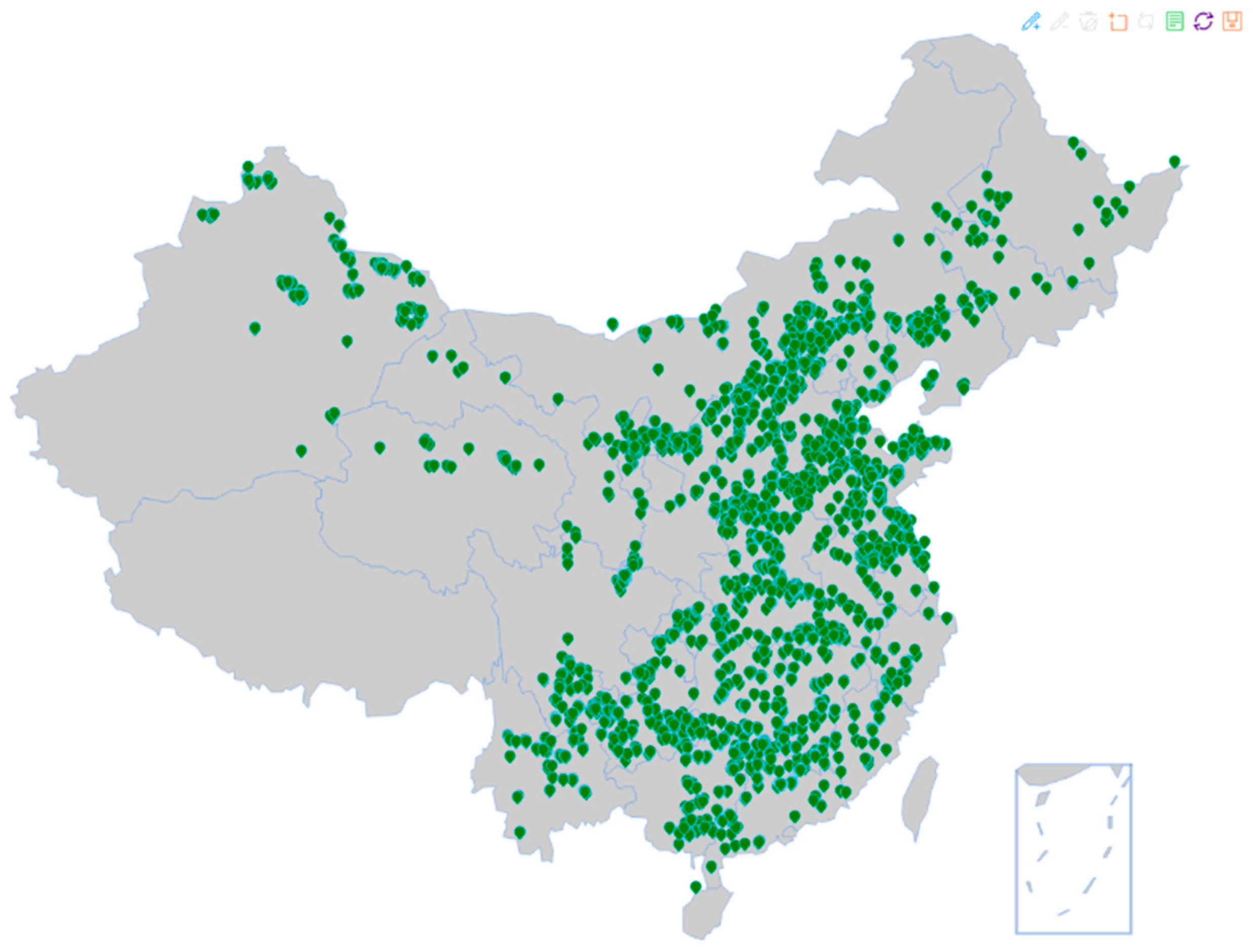
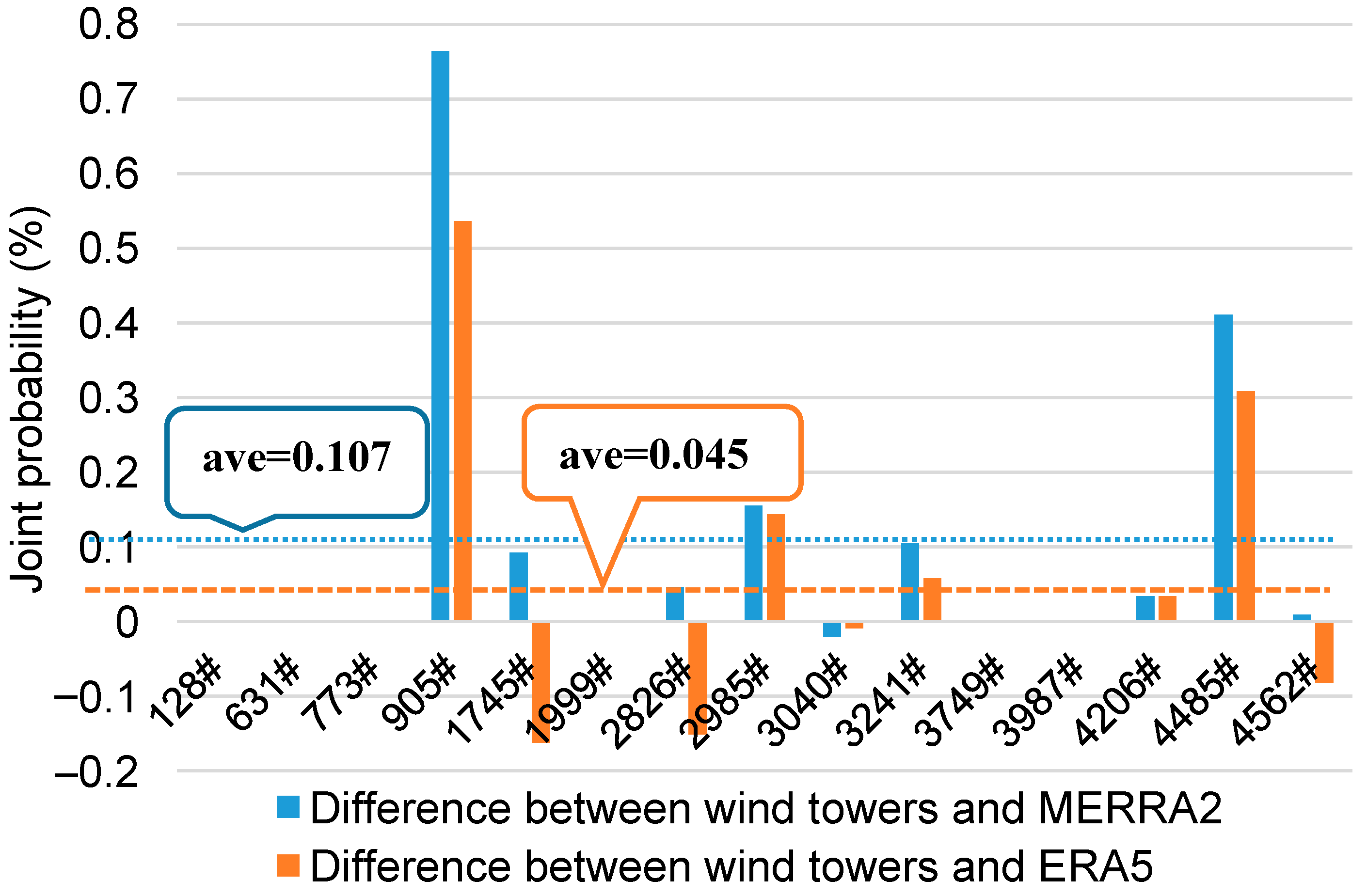
Region	Number of Wind Towers	${\mathit{N}}_{\mathit{T}\mathit{o}\mathit{w}\mathit{e}\mathit{r}>\mathit{E}\mathit{R}\mathit{A}5}$	Minimum Difference (%)	Maximum Difference (%)	${\mathit{N}}_{\left|\mathit{d}\right|>0.5}$
North China	269	21	−0.776	0.372	5
Central China	79	25	−0.489	0.424	0
Northeast China	70	11	−0.536	0.137	1
East China	120	22	−0.333	0.241	0
Northwest China	68	12	−0.501	0.187	1
Total	606	91	--	--	7

. We then count the corresponding differences between the two ways and get the minimum and maximum values. The number of the regions that the absolute values of the difference is greater than 0.5% (denoted as $N_{\left|d\right|>0.5}$) is also listed.

It is seen from Table 4 that only 15% (91/606) of probabilities using wind towers are larger than those using EAR5. For the difference between the two methods, only 1.15% (7/606) of the cases are higher than 0.5%. That is, the joint probability distribution of using ERA5 is very similar to that of using wind towers, so the ERA5 dataset can be used as an effective supplement to improve the representativeness of the joint probability distribution computation. This provides support for analyzing the environmental conditions of the target wind field to be constructed in future engineering applications.

6. Conclusions

To ensure accurate boundary design of DDPM wind generators in engineering applications, this paper proposes a novel environmental condition boundary design method using the extreme joint probability distribution.

Compared to traditional methods of environmental boundaries design which may exceed the operating environmental conditions with lower power density of generator and higher waste of materials, this work formulates the relationship between the design boundaries of wind generator and joint probability of environmental conditions. Accordingly, the wind generator design boundaries can be optimized by blending the LCOE evaluation with multiple scheme selection, so as to formulate a straightforward and feasible scheme for wind engineering. Furthermore, to validate the proposed boundary design method, the Goldwind 3.3-MW DDPMG and five typical wind farms in China are used for case studies. Moreover, some mesoscale model simulation datasets like ERA5 and MERRA2 are analyzed as effective supplements to improve the representativeness of computing the joint probability distribution.

Note that this work mainly focuses on the DDPMG wind generators, so optimizing the design boundaries for other types of wind generators should involve the datasets of their unique characteristics and environmental conditions, whereas the parameter ranges shown in Section 3 should be adjusted accordingly. Moreover, more typical datasets of wind areas beyond China are to be gathered and analyzed to validate and extend the feasibility of the boundary design method. These are topics for upcoming studies.

References

- Caboni, M.; Campobasso, M.; Minisci, E. Wind Turbine Design Optimization under Environmental Uncertainty. J. Eng. Gas Turbines Power Trans. ASME 2016, 138, 082601. [Google Scholar] [CrossRef]
- Simão, M.L.; Sagrilo, L.; Videiro, P. A multi-dimensional long-term joint probability model for environmental parameters. Ocean. Eng. 2022, 255, 111470. [Google Scholar] [CrossRef]
- Dong, J.; Lv, S.; Zhu, Y.; Han, H.; Zhang, G. Research on Wind Power Energy Storage Joint Optimization Operation under the Double Detailed Rules Assessment Taking into Account the Benefits of Green Certificate. Sustainability 2023, 15, 431. [Google Scholar] [CrossRef]
- Toft, H.; Svenningsen, L.; Sørensen, J.; Moser, W.; Thøgersen, M. Uncertainty in wind climate parameters and their influence on wind turbine fatigue loads. Renew. Energy 2016, 90, 352–361. [Google Scholar] [CrossRef]
- Vorpahl, F.; Schwarze, H.; Fischer, T.; Seidel, M.; Jonkman, J. Offshore wind turbine environment, loads, simulation, and design. Wiley Interdiscip. Rev. Energy Environ. 2013, 2, 548–570. [Google Scholar] [CrossRef]
- Dong, S.; Chen, C.; Tao, S. Joint probability design of marine environmental elements for wind turbines. Int. J. Hydrog. Energy 2017, 42, 18595–18601. [Google Scholar] [CrossRef]
- Mirnikjoo, S.; Abbaszadeh, K.; Abdollahi, S. Multiobjective Design Optimization of a Double-Sided Flux Switching Permanent Magnet Generator for Counter-Rotating Wind Turbine Applications. IEEE Trans. Ind. Electron. 2021, 68, 6640–6649. [Google Scholar] [CrossRef]
- Dube, L.; Garner, K.; Kamper, M. Performance of Multi Three-Phase Converter-Fed Non-Overlapping Winding Wound Rotor Synchronous Wind Generator. In Proceedings of the International Conference on Electrical Machines (ICEM), Valencia, Spain, 5–8 September 2022. [Google Scholar]
- Yuan, Z.P.; Li, P.; Li, Z.L.; Xia, J. Data-Driven Risk-Adjusted Robust Energy Management for Microgrids Integrating Demand Response Aggregator and Renewable Energies. IEEE Trans. Smart Grid 2023, 14, 365–377. [Google Scholar] [CrossRef]
- Fingersh, L.; Hand, M.; Laxson, A. Wind Turbine Design Cost and Scaling Model; Technical Report, TP-500-40566; National Renewable Energy Laboratory: Golden, CO, USA, 2006.
- Shields, M.; Beiter, P.; Jake, D.; Nunemaker, A.; Cooperman, P. Duffy, Impacts of Turbine and Plant Upsizing on the Levelized Cost of Energy for Offshore Wind. Appl. Energy 2021, 298, 117189. [Google Scholar] [CrossRef]
- Chen, J.; Wang, F.; Stelson, K. A mathematical approach to minimizing the cost of energy for large utility wind turbines. Appl. Energy 2018, 228, 1413–1422. [Google Scholar] [CrossRef]
- IEC 60034-29; Rotating Electrical Machines-Part 29: Equivalent Loading and Superposition Techniques—Indirect Testing to Determine Temperature Rise. IEC: Geneva, Switzerland, 2008.
- IEC 60034-1; Rotating Electrical Machines-Part 1: Rating and Performance. IEC: Geneva, Switzerland, 2017.
- Hasager, C.; Badger, M.; Nawri, N. Mapping Offshore Winds Around Iceland Using Satellite Synthetic Aperture Radar and Mesoscale Model Simulations. IEEE J. Sel. Top. Appl. Earth Obs. Remote Sens. 2015, 8, 5541–5552. [Google Scholar] [CrossRef] [Green Version]
- Castorrini, A.; Gentile, S.; Geraldi, E.; Bonfiglioli, A. Investigations on offshore wind turbine inflow modelling using numerical weather prediction coupled with local-scale computational fluid dynamics. Renew. Sustain. Energy Rev. 2023, 171, 113008. [Google Scholar] [CrossRef]