Abstract
As an alternative for sustainable transportation and economic development, biofuels are being promoted as renewable and climate-friendly resources of energy which can help to reduce the consumption of fossil fuels, some pollutant emissions and mitigate the climate change impact from transport. With the successful development of the biofuel industry, the location selection for biofuel production plant is one of the major concerns for the governments and policymakers. Finding locations for the construction of new biofuel production plants includes several dimensions of sustainability, including economic, social and environmental; therefore, this selection process can be considered a complex multi-criteria decision-making problem with uncertainty. As an advanced version of fuzzy set, picture fuzzy set (PiFS) is one of the comprehensive tools to handle the uncertainty with the account of truth, abstinence and falsity membership degrees. Thus, this work proposes a new decision-making methodology based on the weighted aggregated sum product assessment (WASPAS) approach and similarity measure with picture fuzzy information. By using picture fuzzy numbers, the proposed methodology can effectively address the uncertain information and qualitative data that often occurs in practical applications. In this methodology, a picture fuzzy similarity measure-based weighting model is proposed to find the criteria weights under picture fuzzy environment. For this purpose, a new similarity measure is introduced to measure the degree of similarity between picture fuzzy numbers. Moreover, the rank of the options is determined based on an integrated WASPAS approach under a PiFS context. To illustrate the effectiveness of the proposed framework, a case study of biofuel production plant location selection is presented from the picture fuzzy perspective. Further, a comparison with existing methods is conducted to test the validity and applicability of the obtained results. The sensitivity analysis is performed with respect to different values of decision parameter, which proves the stability, robustness, and practicality of the proposed approach. The presented picture fuzzy WASPAS approach feasibly enables the policymakers to identify the most desirable location for a biofuel production plant by considering the social, environmental and economic aspects of sustainability.
1. Introduction
Energy is a critical enabler of economic transformation and social wellbeing; therefore, the need for abundant, affordable, secure, safe, and clean energy and its related services is increasing to promote the economic and social growth of the developing countries [1,2]. Increased rate of fossil fuel combustion is one of the major human sources of greenhouse gas (GHG) emissions, acid rain, pollutions and CO2-driven climate change [3,4]. Global demand for energy, food security, environmental degradation and significant weather problems are the most critical issues that are motivating to search for low-carbon alternative fuels at both regional and national levels [5,6].
Biofuels are considered to be one of the renewable and sustainable sources of energy, with the high prospect and potential of reducing carbon emissions, as well as mitigating the climate change [7]. The production of biofuels from a sustainability perspective is an important and critical process for conserving biodiversity, ensuring global energy security, reducing environmental issues and improving economic and social aspects, especially in developing countries [8,9,10]. Transportation and agricultural industries are one of the main consumers of fossil fuels and a prime contributor to environmental pollution, which can be reduced by replacing biofuels. There are several complex aspects in the production of biofuels. One such aspect is the placement of biofuel production plants (BPPs), which faces challenges at all phases of the production and logistics planning [11].
The assessment of BPP locations involves numerous criteria which are strongly related to the triple bottom line (TBL) theory of sustainability [8,9]. Thus, it is essential to evaluate the criteria based on the social, environmental and economic aspects of sustainability. In the literature, few studies have been developed to assess the locations for BPP. In this context, Bai et al. [12] focused their study on the planning and assessment of biorefinery plant locations. Zhang et al. [13] suggested a two-phase multiple attribute methodology for selecting the suitable location for BPP. In that study, they used a geographic information system with a minimum transportation cost model to identify the best location. Duarte et al. [11] designed a mixed integer linear programming-based optimization tool that considers the process design and configuration of the supply chain during BPP location selection. Their study was implemented on a real case study of second-generation BPP location selection in Colombia. Kheybari et al. [9] developed a multi-criteria decision support framework based on best worst method. Further, they implemented their framework on a case study of bioethanol location selection in Iran. Najafi et al. [14] firstly identified the relevant sustainability indicators for BPP location selection. They used the Shannon entropy model to derive the criteria weights and the additive ratio assessment method to find the ranking of locations for biodiesel fuel production plants. Nordin et al. [15] presented a spatial optimization model for evaluating the locations of agricultural BPP and feedstocks in Sweden. Moreover, they provided implications for animal fodder availability, renewable energy and climate emissions.
The theory of fuzzy set (FS) [16] is characterized by the truth/membership degree of the function. After the pioneering work of Zadeh [16], various extensions of FS have been introduced to express the uncertain information of real-life problems [17,18,19,20,21,22]. In FSs, the truth degree (TD) is defined on interval [0, 1], while the falsity degree (FD) defines its complement. However, this statement does correlate with human behavior in practical examples. To evade the concerns of FSs, the notion of the intuitionistic fuzzy set (IFS) [23] has been proposed with three parameters: the TD, the FD and the indeterminacy degree (ID) satisfying the condition that the sum of TD and FD is ≤1. Since its appearance, many theories and applications have been discussed in the literature [24,25,26].
In the process of voting, the voters present multiple-selection opinions as follows: ‘yes’, ‘no’, ‘abstain’, and ‘refusal’. This case cannot be exactly described by FSs [16], IFSs [23], Pythagorean fuzzy sets (PFSs) [27], Fermatean fuzzy sets (FFSs) [28] or hesitant fuzzy sets (HFSs) [29]. This specific type of information is frequently used in several real-life problems including survey analysis, voting system and data analysis, where voters may be separated into the aforementioned four classes. To deal with such situations, Cuong [30,31] pioneered the notion of the picture fuzzy set (PiFS) theory, which contains the degrees of truth, abstinence and falsity such that their sum cannot exceed the unit interval. The concept of PiFS expresses the uncertainty and non-determinism more efficiently than FS, IFS, PFS, FFS and HFS. Many theories and applications have been presented in the context of PiFS [32]. For instance, Jana et al. [33,34] proposed a series of Hamacher and Dombi aggregation operators to aggregate the picture fuzzy information. A new dynamic programming algorithm-based picture fuzzy clustering model has been proposed for large-scale group decision-making problems [35]. Due to the advantages of PiFSs, Simic et al. [36] extended the classical COmbinative Distance-Based ASsessment (CODAS) approach under a PiFS environment and applied it for solving vehicle shredding facility location with multiple criteria. Singh and Kumar [37] integrated the quality function deployment with picture fuzzy numbers and proposed a hybrid multi-criteria group decision-making framework. Wei et al. [38] studied the picture fuzzy bidirectional projection method for solving group decision-making problems with multiple tangible and intangible criteria. A hybrid picture fuzzy similarity measure-based ranking model has been developed for assessing projects from a sustainability perspective [39]. Fetanat and Tayebi [40] proposed a hybrid decision support system by using the PiFS concept to prioritize the petroleum refinery effluents. A strategy-based picture fuzzy conversion model has been developed by Zhao et al. [41], which considers the evidential reasoning concept with picture fuzzy information.
Despite the fact that there are several MCDM methods in the literature, the investigators generally opt for a method that works well with the type and intricacy of the problem considered. As one of the newly developed approaches, weighted aggregated sum product assessment (WASPAS) [42] optimizes the weighted aggregated functions and ranks the options according to a compromise solution. The WASPAS method has been applied for a variety of purposes, such as sustainable project portfolio selection [43], foreign direct investment assessment [44], hair mask product selection [45], etc. The classical WASPAS method has been extended from q-rung orthopair fuzzy perspective. Moreover, they utilized their method for the assessment of alternative fuel technologies under an uncertain environment [46]. Mishra et al. [47] assessed the biomass crops for biofuel production by using a new single-valued neutrosophic WASPAS methodology. Wei et al. [48] extended the WASPAS method by using the reducible weighted Maclaurin symmetric mean operator and PFS theory. Further, they presented the application of the WASPAS method in teaching quality assessment. Chakraborty and Saha [49] combined the WASPAS approach with fuzzy analytic hierarchy process (AHP) for assessing the healthcare waste technology selection problem. Utilizing the uncertainty concepts, Ebadzadeh et al. [50] proposed a fuzzy WASPAS approach for assessing the environmental risks of the petrochemical industry. In the context of PiFSs, Simic et al. [51] and Senapati and Chen [52] introduced the hybrid picture fuzzy WASPAS approaches with applications in last-mile delivery mode assessment and an air-conditioning system selection, respectively. Unfortunately, there has been no study extending the similarity measure-based WASPAS method with PiFSs to solve BPP location selection problem in the literature.
Due to the broader range of PiFSs in handling the vague information, the current work focuses on the development of a new decision support system under the PiFS context and applied for assessing the locations for BPP construction. The decision-making methods assist the “decision-making experts (DMEs)” to make an optimal decision [45]. Some MCDM methods have been developed to solve the BPP location selection problem [8,9,10,11,12,13], but these studies have some drawbacks:
- (i)
- unable to derive the criteria weights;
- (ii)
- unable to express the vague information.
Inspired by the concept of WASPAS, this study proposes an integrated WASPAS method with picture fuzzy information, in which the weights of the criteria are derived through the PiFSM-based model. A few studies [51,52] simply extended the classical WASPAS to PiFSs setting, but they did not consider the significance of DMEs and criteria weights during the process of decision making. To the best of the authors’ knowledge, none of the previous studies have addressed the BPP location selection problem using an integrated picture fuzzy similarity measure-based WASPAS approach.
Based on the above discussions, the key contributions of this work are listed as:
- By means of literature survey and interview with experts, a comprehensive index system is presented to evaluate the key criteria for BPP locations’ assessment.
- A novel formula is presented to derive the DMEs’ weights.
- A novel criteria weight-determining model is developed based on PiFSM. For this purpose, we introduce a new similarity measure for PiFSs.
- A modified WASPAS method based on the combination of new weight-determination process and picture fuzzy information is introduced for solving BPP location selection from sustainability perspective.
- To prove the effectiveness of the present WASPAS approach, an empirical case study of BPP location selection is presented within the context of PiFSs.
The rest of this study is arranged as follows: Section 2 presents the basic concepts and then introduces a new SM for PiFSs. Section 3 establishes a hybrid decision support system for making decisions under picture fuzzy environment. Section 4 implements the proposed system on a case study of BPP location selection problem of Ahmedabad, India. In addition, this section further discusses the sensitivity and comparative analyses to confirm the validity of obtained results. Section 5 discusses the findings and scope for further research.
2. Literature Review
In the current section, we firstly discuss the fundamental definitions related to this study. Further, we introduce an SM, which quantifies the degree of similarity between PiFSs.
2.1. Basic Concepts
Definition 1.
A PiFS H on a finite universal setis mathematically expressed as [30,31]
where and denote the degrees of truth, abstinence and falsity membership of in H, respectively, with the condition. For each the degree of refusal membership is computed by
Definition 2.
Letbe a picture fuzzy number (PiFN). Then, the score and accuracy functions are represented by Equations (1) and (2), respectively [53].
Example 1.
For any two PiFNsandthe score function of H1 isand the score function of H2 is therefore, the order of the PiFNs is
Example 2.
For any two PiFNsandthe score function of H1 isand the score function of H2 istherefore, H1 = H2. In this case, we are unable to discriminate the order of H1 and H2. Then, we compute accuracy values of H1 and H2, which areand respectively. Thus, the order of given PiFNs is
Definition 3
([30,31,54]). Let and be two PiFNs. Then, the operational laws on PiFNs are defined as
- (i)
- (ii)
- (iii)
- (iv)
- (v)
Example 3.
Letandbe two PiFNs. Then the operational laws given by Definition 3are computed as
- (i)
- and
- (ii)
- (iii)
- (iv)
- (v)
Definition 4
([55]). Let A real-valued function is said to be a PiFSM if it satisfies the following postulates:
- (s1).
- (s2).
- (s3).
- if and only if
- (s4).
- Forifthenand
2.2. Picture Fuzzy Similarity Measure
SM, as one of the well-known information measures, is widely applied for data mining, medical diagnosis, pattern recognition, etc. As PiFS considers the wider range of fuzzy information, some authors have proposed some SMs to assess the degree of similarity between PiFSs [55]. For instance, Luo and Zhang [56] analyzed the drawbacks of the existing picture fuzzy similarity measures (PiFSMs). To overcome their drawbacks, the authors have introduced a new similarity measure (SM) for PiFSs with an application in pattern recognition problems. Singh and Ganie [57] proposed some new SMs for PiFSs with applications in several areas. Khan et al. [58] highlighted the counter-intuitive cases of several existing PiFSMs and further proposed a bi-parametric PiFSM and distance measure for a medical diagnosis application. Tian et al. [39] proposed a PiFSM and used it to develop a decision-making algorithm for solving projects evaluation from sustainability viewpoints.
The exponential function has an advantage over the polynomial, trigonometric and logarithmic functions. Unfortunately, there is no study regarding the exponential-function-based PiFSM. Inspired by this concept, we propose a SM for PiFSs and further use it to derive the numeric weights of criteria.
For we present a new PiFSM in accordance with [59,60]
Lemma 1.
Ifthenand.
Proof.
The derivative of is which is negative; therefore, the given function is decreasing in Thus, and . For more details, please see ref. [59]. □
Theorem 1.
The functiongiven by Equation (4), is a valid similarity measure for PiFS.
Proof.
To prove this theorem, we have to verify the properties (s1)–(s4) of Definition 4.
(s1). For where and
therefore, Thus, in accordance with Lemma 1, we have .
(s2). It is obvious from Equation (4).
(s3). From Equation (4), if then . Conversely, let . Then, from Equation (4), we obtain
It implies that
Hence,
(s4). Given that then and Then,
Consequently, with Lemma 1, we have Similarly, we can verify that □
3. Integrated Picture Fuzzy WASPAS (PiF-WASPAS) Method for MCDM Problems
In this section, an integrated method is introduced to tackle the MCDM problems from a picture fuzzy perspective, which is based on the classical WASPAS approach. The proposed method is developed to handle the MCDM problems with unknown criteria and DMEs’ weights. In the proposed framework, a novel formula is presented to compute criteria weights based on PiFSM. With the use of PiFSs, the DMEs provide more flexibility in expressing their preferences under uncertain situations. The steps of PiF-WASPAS method are as follows:
Step 1: Construct the linguistic decision matrix (LDM).
In the MCDM problem, consider a set of options with respect to a set of criteria Let be a set of ‘l’ DMEs which give his/her opinions on each option Pi under the criteria in forms of PiFNs. Let be the LDM provided by the DMEs, where denotes the performance value of an option under each criterion in terms of linguistic values (LVs) given by expert.
Step 2: Determining the DMEs weights.
In the process of group decision-making, the significance of DMEs’ weights is an important concern. For the assessment of kth expert, let be the PiFN; then, the formula for kth DME’s weight is evaluated by
Clearly, and .
Step 3: Create an aggregated picture fuzzy decision matrix (A-PiFDM).
To aggregate the group DMEs’ opinions, the picture fuzzy weighted averaging operator (PiFWAO) [28] is used on PiFDM. Let be the A-PiFDM, where
Step 4: Calculate the weights of the criteria.
Suppose is the weight of the criterion set with and To find the criteria weights, we present a PiFSM-based formula, given as
Step 5: Normalize the A-PiFDM.
The normalized A-PiFDM from A-PiFDM is computed, where
Here, and denote the benefit and cost types of criteria, respectively.
Step 6: Determine the measure of weighted sum model (WSM) for each option as follows:
where i = 1, 2, …, m.
Step 7: Evaluate the measure of weighted product model (WPM) for each option as follows:
where i = 1, 2, …, m.
Step 8: Evaluate the integrated measure of the WASPAS for each option as follows:
wherein ‘’ signifies the coefficient of decision mechanism, where (when and the WASPAS is altered into the WPM and the WSM, respectively).
Step 9: According to the values of where i = 1, 2, …, m, rank the given alternatives.
Step 10: End.
4. Case Study: Biofuel Production Plant (BPP) Location Selection
For this case study, we selected Ahmedabad, the largest city in the state of Gujarat. Ahmedabad is a lively business city and rising center of the education, information technology and manufacturing sectors. To show the performance of the present hybrid methodology, we implement it on a case study of BPP location selection problem in Ahmedabad, Gujarat. An Indian company wants to establish a new BPP in Ahmedabad but it does not have any proper procedure for establishment. In this study, we focus on the development of a new robust approach for BPP construction companies which will assist the DMEs to evaluate the most suitable location for BPP.
To select the most suitable BPP, a panel of four DMEs has been created who have more than 10 years’ experience in the field of sustainability and ecological planning. After preliminary analysis, this team has considered five prospective locations, which are location 1 (P1), location 2 (P2), location 3 (P3), location 4 (P4), and location 5 (P5). The key idea of the study is to firstly identify the indicators/criteria for locating BPP. Thirteen criteria are considered and described in Table 1.

Table 1.
Considered criteria for BPP location selection.
Steps 1–3:Table 2 (adopted from [37]) depicts the importance of the DMEs and criteria in the form of LVs and then converted into PiFNs. Table 3 presents the DMEs’ weights with the score degree-based model using Table 2 and Equation (5). Table 4 describes the importance of DMEs as LDM to evaluate the BPP location options concerning each criterion. The LDM offered by four DMEs have been combined utilizing Equation (6) into an A-PiFDM considering the significance ratings of DMEs, which are provided in Table 5.
Table 2.
Linguistic ratings for weighting the DMEs, BPP locations [61].
Table 3.
Weights of DMEs for evaluation of the BPP locations.
Table 4.
LDM created by DMEs for BPP location selection.
Table 5.
A-PiFDM for BPP location selection.
Step 4: From the proposed PiF similarity measure-based model, we find the weights of the criteria by using Equation (8), which are given as follows (see Figure 1):
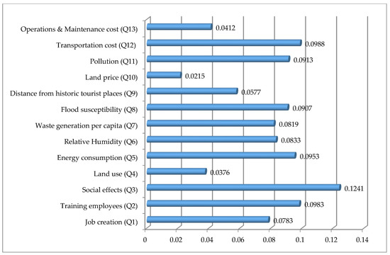
Figure 1.
Significance values/weight of criteria for BPP location selection.
Here, Figure 1 presents the weights of the different indicators/criteria for locating BPP with respect to some goals. Social effects (Q3) with a weight value of 0.1241 have turned out to be the most important criterion for locating BPP. Transportation cost (Q12) with a weight value of 0.0988 is the second most important criterion for locating BPP. Training employees (Q2) ranks third, with a significance value of 0.0983; energy consumption (Q5) ranks fourth, with a significance value of 0.0953; and pollution (Q11), with a significance value of 0.0913,ranks as the fifth most important criterion for locating BPP; others are considered crucial criteria for BPP location selection.
Step 5: Since the criteria Q1,Q2, Q3 and Q9 are of benefit types and the others are non-cost types, using Equation (8) and Table 5, the normalized A-PiFDM is presented in Table 6.
Table 6.
Normalized A-PiFDM for BPP location selection.
Steps 6–9: Using Table 6 and Equations (9) and (10), the measures of WSM and WPM are evaluated. Subsequently, in accordance with Equation (11), the utility degree (at is computed and shown in Table 7. From Table 7, the prioritization order of BPP locations is P2 P1 P5 P3 P4; therefore, P2 is the most desirable location for BPP location selection.
Table 7.
Utility degree of each option using the PiF-WASPAS method.
5. Discussion
This section firstly discusses the effect of the parameters on the obtained outcomes and further discusses the comparative study based on the proposed and existing approaches under a PiFS context.
5.1. Sensitivity Analysis
Here, different values of are considered for investigation. This assessment is performed to illustrate the performance of the present WASPAS methodology. The variation of values can assist us in discussing the sensitivity of the introduced methodology from WSM to WPM. From Table 8 and Figure 2, the rank of locations over different criteria for BPP location selection is presented from different parameter values. Hence, it is established that the desirable location for BPP location selection is dependent on and sensitive to criteria weights. According to Figure 2, location (P2) has obtained the first rank for each parameter value, location (P4) has obtained the last rank for BPP location selection. Based on the aforementioned study, it is observed that using the diverse values of the parameters will enhance the permanence of the PiF-WASPAS methodology.
Table 8.
The utility degree of option over different parameter (λ) values.
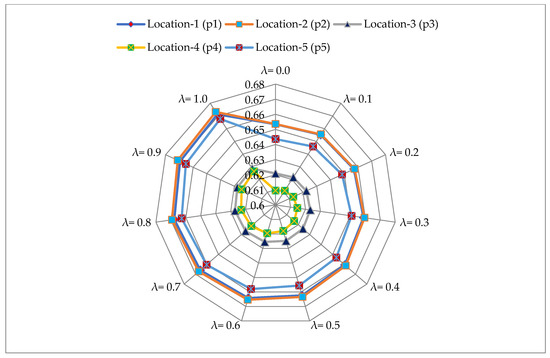
Figure 2.
Sensitivity analysis test on decision parameter λ values for each option.
5.2. Comparative Study
Here, a comparative study is conducted to show the effectiveness of the obtained outcomes over the existing picture fuzzy information-based MCDM approaches. For this purpose, we compare the proposed method with some of the existing methods, including the PiF-COPRAS method [62], the PiF-VIKOR method [63] and the ranking method [64].
5.2.1. PiF-COPRAS [62]
This method involves the following steps:
Steps 1–4: Similar to proposed model.
Step 5: Sum of the ratings for benefit and cost types criteria.
Let and be the aggregated ratings of each option with benefit and cost types of criteria, respectively. Then, we utilized Equations (12) and (13) to evaluate the values of and
Step 6: The relative degree (RD) of each option is determined as
Step 7: The utility degree (UD) of each option is computed as
The PiF-COPRAS method is implemented on the same case study of BPP location selection problem. The overall results of PiF-COPRAS are shown in Table 9. From Table 5 and Equations (12)–(15), the RD and UD of each option are obtained. Based on the UD (see Table 9), option (P2) is found to be the most suitable choice with maximum RD (0.4122) for prioritizing the BPP location.
Table 9.
The results of PiF-COPRAS model for BPP location.
5.2.2. PiF-VIKOR [63]
Steps 1–4: Same as previous model.
Step 5: The ideal and anti-ideal solutions are determined under a PiFS context.
Step 6: In accordance with the proposed projection measure and A-PiFDM, we compute the group utility (GU) and the individual regret (IR) over each option Pi, which are given by
where such that Similarly, we can compute [63].
The compromise score (CS) (ei) for each option is computed as
Step 7: Prioritize the candidates.
Corresponding to the values of GU, IR and CS, determine the ranking order of the given options.
Step 8: Determination of the compromise solution.
Consider the candidate Pi as a CS in accordance with e1 (the least among ei values) if:
(R1): The option Pi has an acceptable improvement, i.e., wherein m determines the number of alternatives.
(R2): The alternative Pi is stable in the process of decision making, i.e., it is also best ranked by gi or ri.
If anyone of the conditions is not held, then a group of CSs is proposed, which consists of:
- (a)
- Alternatives P1 and P2 if only the condition (R2) is not held.
- (b)
- Alternatives P1, P2, P3, …,Pk if (R1) is not satisfied; and Pk is evaluated by the expression
We implement the PiF-VIKOR approach on the aforementioned case study of BPP location selection problem. Therefore, the best and worst values of the BPP locations are computed as {(0.773, 0.057, 0.115), (0.777, 0.050, 0.118), (0.835, 0.050, 0.111), (0.297, 0.060, 0.610), (0.269, 0.060, 0.638), (0.253, 0.050, 0.647), (0.244, 0.060, 0.664), (0.274, 0.060, 0.633), (0.777, 0.050, 0.166), (0.224, 0.050, 0.675), (0.227, 0.050, 0.673), (0.200, 0.050, 0.700), (0.298, 0.060, 0.609)} and {(0.629, 0.057, 0.245), (0.639, 0.070, 0.284), (0.590, 0.082, 0.272), (0.352, 0.050, 0.546), (0.428, 0.060, 0.474), (0.400, 0.069, 0.508), (0.397, 0.073, 0.512), (0.470, 0.050, 0.428), (0.636, 0.050, 0.245), (0.256, 0.050, 0.644), (0.415, 0.061, 0.488), (0.397, 0.073, 0.512), (0.372, 0.057, 0.530)} (Wang et al., 2018).
Using Equations (15)–(17), the values of gi, ri and eibased on the projection measure are derived and shown in Table 10. In accordance with these obtained values, the prioritization order of BPP location selection is determined (see Table 10). Minimum value of ei determines the best BPP location, i.e., P3.
Table 10.
The values of gi, ri and ei for the evaluation of BPP location.
5.2.3. Ranking Method [64]
Steps 1–5: Same as previous model
Step 6: Estimate the collective value of each alternative using Equation (9).
Step 7: Find the score values of overall aggregated values.
Step 8: As per the decreasing score values, prioritize the options.
We apply the Garg’s method on the aforementioned BPP location selection problem. In this regard, we obtain the collective values as c1 = (0.646, 0.057, 0.243), c2 = (0.652, 0.058, 0.244), c3 = (0.604, 0.061, 0.284), c4 = (0.600, 0.057, 0.288) and c5 = (0.658, 0.060, 0.260).
Step 9: The score values of the aggregated values ci(i = 1, 2, 3, 4, 5) are (c1) = 0.6728, (c2) = 0.6749, (c3) = 0.6295, (c4) = 0.6274 and (c5) = 0.6689.
Step 10: Since (c2) > (c1) > (c5) > (c3) > (c4), we have P2 P1 P5 P3 P4. Hence, the best location for BPP is P2.
From Table 11, it can easily be determined that option P2 has the best significance value in all the methods except in the PiF-VIKOR [63] model. In comparison with the existing procedures, the main advantages of the introduced PiF-WASPAS methodology are as follows (see Figure 3):
Table 11.
Comparison of the parameters with the existing methodologies.
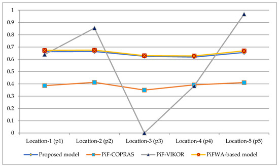
Figure 3.
Comparison of degree of utility/closeness index of each manufacturing firm with various methods.
- In PiF-COPRAS [62] and Garg’s method [64], the overall compromise/collective scores are obtained with the use of picture fuzzy weighted averaging operators. In PiF-VIKOR [62], the compromise score is estimated based on the projection measure. The proposed PiF-WASPAS is a novel, robust, utility-based method. This approach is an integration of WPM and WSM. The precision of this approach is stronger than that of WPM and WSM. WASPAS enables the attainment of the maximum precision of assessment, utilizing the introduced methodology for optimizing the weighted AOs.
- For the PiF-COPRAS method [62], the decision expert’s weight is assumed and PiF-VIKOR [63] and Garg’s method [64] do not consider the decision expert’s weight. In the present method, each decision expert is assigned equal weight value. In addition, the computation process of the PiF-WASPAS method is simpler, and therefore, the accuracy and reliability of the results are higher.
- In PiF-COPRAS [62], the CRITIC tool is applied to find only the objective weight of the criteria. In Garg’s method [64], the weight of a criterion is randomly chosen. In the PiF-VIKOR approach [63], the entropy-based model is used to evaluate the objective weight of criteria. In the developed methodology, a procedure based on the similarity measure is applied to compute the objective weight of criteria owing to its simplicity and smaller number of calculation steps, which proves that the proposed method is more flexible, efficient, and sensible.
However, the method proposed in this study has some limitations:
- This method ignores the subjective and objective weights of criteria.
- In this method, we consider only benefit and cost types of criteria and ignore the target-based criteria.
6. Conclusions
In this paper, we presented a hybrid decision making framework for evaluating and prioritizing the BPP location from the uncertainty and sustainability perspectives. In this regard, first, a new similarity measure has been introduced for PiFSs. Next, we have incorporated the WASPAS approach with PiFSM and a score degree-based model within the environment of PiFSs. The criteria weights have been derived through the PiFSM-based weighting formula. Further, the proposed method has been implemented on a case study of BPP locations’ assessment, which shows the applicability and effectiveness of the presented decision-making framework. The criteria evaluation index for BPP location selection is presented, which contains three aspects of sustainability, namely social, environmental and economic (Figure 4). These three dimensions consist of three, six and four criteria, respectively, and the weights of all criteria are derived using the proposed weighting model. The calculation result shows that the alternative ‘location (P2)’ is the most suitable choice for a given case study based on available data. Further, sensitivity and comparative analyses have been discussed to confirm the results acquired by the proposed PiF-WASPAS model. The presented method incorporates the benefits of the picture fuzzy numbers and the WASPAS technique. In this study, the picture fuzzy numbers can express uncertain and incomplete information that inherently exists in the BPP location section decision-making problem, while WASPAS offers formulation flexibility and simple calculations. The main benefits of the presented framework are the ease of computation in the picture fuzzy background and utilizing a model for deriving more reasonable weights of indicators.
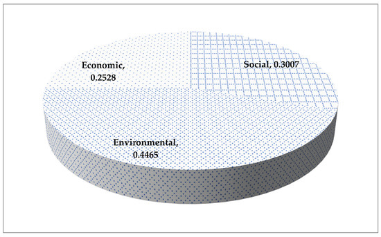
Figure 4.
Depiction of the significance degrees of different aspects of sustainability.
In the future, it would be exciting to improve the limitations of the present study by proposing some new methods, such as operational competitiveness rating (OCRA), double normalization-based multiple aggregation (DNMA), gained lost dominance score (GLDS), etc. In addition, this study can be extended to q-rung orthopair rough fuzzy sets, interval-valued picture fuzzy sets, and interval-valued q-rung orthopair rough fuzzy sets by developing new aggregation operators to aggregate the DMEs’ opinions, and can be applied to alternative social baking systems, transportation management, plastic waste recycling technology selection, green energy projects’ assessment and vertical farming technology evaluation.
Author Contributions
Methodology, P.R.; Validation, J.L.; Formal analysis, I.M.H., F.C. and P.R.; Investigation, J.L.; Writing—original draft, I.M.H.; Supervision, F.C. and S.G.; Project administration, S.G. All authors have read and agreed to the published version of the manuscript.
Funding
This research is funded by Researchers Supporting Project number (RSP2023R389), King Saud University, Riyadh, Saudi Arabia.
Institutional Review Board Statement
Not applicable.
Informed Consent Statement
Not applicable.
Data Availability Statement
Not applicable.
Conflicts of Interest
The authors declare no conflict of interest.
References
- Yücenur, G.N.; Çaylak, Ş.; Gönül, G.; Postalcıoğlu, M. An integrated solution with SWARA & COPRAS methods in renewable energy production: City selection for biogas facility. Renew. Energy 2020, 145, 2587–2597. [Google Scholar]
- Zhang, G.; Shi, Y.; Maleki, A.; Rosen, M.A. Optimal location and size of a grid-independent solar/hydrogen system for rural areas using an efficient heuristic approach. Renew. Energy 2020, 156, 1203–1214. [Google Scholar] [CrossRef]
- Zhu, B.; Su, B.; Li, Y. Input-output and structural decomposition analysis of India’s carbon emissions and intensity, 2007/08–2013/14. Appl. Energy 2018, 230, 1545–1556. [Google Scholar] [CrossRef]
- Trappey, A.J.C.; Trappey, C.V.; Lin, G.Y.P.; Chang, Y.-S. The analysis of renewable energy policies for the Taiwan Penghu island administrative region. Renew. Sustain. Energy Rev. 2012, 16, 958–965. [Google Scholar] [CrossRef]
- Paletto, A.; Bernardi, S.; Pieratti, E.; Teston, F.; Romagnoli, M. Assessment of environmental impact of biomass power plants to increase the social acceptance of renewable energy technologies. Heliyon 2019, 5, e02070. [Google Scholar] [CrossRef] [PubMed]
- Cai, W.; Li, X.; Maleki, A.; Pourfayaz, F.; Rosen, M.A.; Nazari, M.A.; Bui, D.T. Optimal sizing and location based on economic parameters for an off-grid application of a hybrid system with photovoltaic, battery and diesel technology. Energy 2020, 201, 117480. [Google Scholar] [CrossRef]
- Benti, N.E.; Aneseyee, A.B.; Geffe, C.A.; Woldegiyorgis, T.A.; Gurmesa, G.S.; Bibiso, M.; Asfaw, A.A.; Milki, A.W.; Mekonnen, Y.S. Biodiesel production in Ethiopia: Current status and future prospects. Sci. Afr. 2023, 19, e01531. [Google Scholar] [CrossRef]
- Ghaderi, H.; Pishvaee, M.S.; Moini, A. Biomass supply chain network design: An optimization-oriented review and analysis. Ind. Crops Prod. 2016, 94, 972–1000. [Google Scholar] [CrossRef]
- Kheybari, S.; Kazemi, M.; Rezaei, J. Bioethanol facility location selection using best-worst method. Appl. Energy 2019, 242, 612–623. [Google Scholar] [CrossRef]
- Ng, R.T.L.; Maravelias, C.T. Design of biofuel supply chains with variable regional depot and biorefinery locations. Renew. Energy 2017, 100, 90–102. [Google Scholar] [CrossRef]
- Duarte, A.E.; Sarache, W.A.; Costa, Y.J. A facility-location model for biofuel plants: Applications in the Colombian context. Energy 2014, 72, 476–483. [Google Scholar] [CrossRef]
- Bai, Y.; Hwang, T.; Kang, S.; Ouyang, Y. Biofuel refinery location and supply chain planning under traffic congestion. Transp. Res. Part B Methodol. 2011, 45, 162–175. [Google Scholar] [CrossRef]
- Zhang, F.; Johnson, D.M.; Sutherland, J.W. A GIS-based method for identifying the optimal location for a facility to convert forest biomass to biofuel. Biomass Bioenergy 2011, 35, 3951–3961. [Google Scholar] [CrossRef]
- Najafi, F.; Sedaghat, A.; Mostafaeipour, A.; Issakhov, A. Location assessment for producing biodiesel fuel from Jatropha Curcas in Iran. Energy 2021, 236, 121446. [Google Scholar] [CrossRef]
- Nordin, I.; Elofsson, K.; Jansson, T. Optimal localisation of agricultural biofuel production facilities and feedstock: A Swedish case study. Eur. Rev. Agric. Econ. 2022, 49, 910–941. [Google Scholar] [CrossRef]
- Zadeh, L.A. Fuzzy sets. Inf. Control 1965, 8, 338–353. [Google Scholar] [CrossRef]
- Rico, N.; Huidobro, P.; Bouchet, A.; Diaz, I. Similarity measures for interval-valued fuzzy sets based on average embeddings and its application to hierarchical clustering. Inf. Sci. 2022, 615, 794–812. [Google Scholar] [CrossRef]
- Debnath, K.; Roy, S.K. Power partitioned neutral aggregation operators for T-spherical fuzzy sets: An application to H2refuelling site selection. Expert Syst. Appl. 2023, 216, 119470. [Google Scholar] [CrossRef]
- Mishra, A.R.; Rani, P.; Cavallaro, F.; Mardani, A. A similarity measure-based Pythagorean fuzzy additive ratio assessment approach and its application to multi-criteria sustainable biomass crop selection. Appl. Soft Comput. 2022, 125, 109201. [Google Scholar] [CrossRef]
- Seker, S.; Aydin, N. Fermatean fuzzy based Quality Function Deployment methodology for designing sustainable mobility hub center. Appl. Soft Comput. 2023, 134, 110001. [Google Scholar] [CrossRef]
- Sharma, H.K.; Roy, J.; Kar, S.; Prentkovskis, O. Multi criteria evaluation framework for prioritizing Indian railway stations using modified rough AHP-Mabac method. Transp. Telecommun. J. 2018, 19, 113–127. [Google Scholar] [CrossRef]
- Sharma, H.K.; Majumder, S.; Biswas, A.; Prentkovskis, O.; Kar, S.; Skačkauskas, P. A Study on Decision-Making of the Indian Railways Reservation System during COVID-19. J. Adv. Transp. 2022. [Google Scholar] [CrossRef]
- Atanassov, K.T. Intuitionistic fuzzy sets. Fuzzy Sets Syst. 1986, 20, 87–96. [Google Scholar] [CrossRef]
- Tripathi, D.K.; Nigam, S.K.; Rani, P.; Shah, A.R. New intuitionistic fuzzy parametric divergence measures and score function-based CoCoSo method for decision-making problems. Decis. Mak. Appl. Manag. Eng. 2022. [Google Scholar] [CrossRef]
- Xie, D.; Xiao, F.; Pedrycz, W. Information quality for intuitionistic fuzzy values with its application in decision making. Eng. Appl. Artif. Intell. 2022, 109, 104568. [Google Scholar] [CrossRef]
- Pandey, K.; Mishra, A.R.; Rani, P.; Ali, J.; Chakrabortty, R. Selecting features by utilizing intuitionistic fuzzy Entropy method. Decis. Mak. Appl. Manag. Eng. 2023. [Google Scholar] [CrossRef]
- Yager, R.R. Pythagorean membership grades in multicriteria decision making. IEEE Trans. Fuzzy Syst. 2014, 22, 958–965. [Google Scholar] [CrossRef]
- Senapati, T.; Yager, R.R. Fermatean fuzzy sets. J. Ambient. Intell. Humaniz. Comput. 2020, 11, 663–674. [Google Scholar] [CrossRef]
- Torra, V. Hesitant fuzzy sets. Int. J. Intell. Syst. 2010, 25, 529–539. [Google Scholar] [CrossRef]
- Cuong, B.C. Picture fuzzy sets-first results. Part 1. In Neuro-Fuzzy Systems with Applications Seminar; Institute of Mathematics: Hanoi, Vietnam, 2013. [Google Scholar]
- Cuong, B.C. Picture fuzzy sets-first results. Part 2. In Neuro-Fuzzy Systems with Applications Seminar; Institute of Mathematics: Hanoi, Vietnam, 2013. [Google Scholar]
- Dutta, P.; Ganju, S. Some aspects of picture fuzzy set. Trans. A. Razmadze Math. Inst. 2018, 172, 164–175. [Google Scholar] [CrossRef]
- Jana, C.; Pal, M. Assessment of enterprise performance based on picture fuzzy hamacher aggregation operators. Symmetry 2019, 11, 75. [Google Scholar] [CrossRef]
- Jana, C.; Senapati, T.; Pal, M.; Yager, R.R. Picture fuzzy Dombi aggregation operators: Application to MADM process. Appl. Soft Comput. 2019, 74, 99–109. [Google Scholar] [CrossRef]
- Pan, X.; Wang, Y.; Chin, K.-S. Dynamic programming algorithm-based picture fuzzy clustering approach and its application to the large-scale group decision-making problem. Comput. Ind. Eng. 2021, 157, 107330. [Google Scholar] [CrossRef]
- Simic, V.; Karagoz, S.; Deveci, M.; Aydin, N. Picture fuzzy extension of the CODAS method for multi-criteria vehicle shredding facility location. Expert Syst. Appl. 2021, 175, 114644. [Google Scholar] [CrossRef]
- Singh, A.; Kumar, S. Picture fuzzy set and quality function deployment approach based novel framework for multi-criteria group decision making method. Eng. Appl. Artif. Intell. 2021, 104, 104395. [Google Scholar] [CrossRef]
- Wei, G.; Zhang, S.; Lu, J.; Wu, J.; Wei, C. An Extended Bidirectional Projection Method for Picture Fuzzy MAGDM and Its Application to Safety Assessment of Construction Project. IEEE Access 2019, 7, 166138–166147. [Google Scholar] [CrossRef]
- Tian, C.; Peng, J.-J.; Zhang, S.; Wang, J.-Q.; Goh, M. A sustainability evaluation framework for WET-PPP projects based on a picture fuzzy similarity-based VIKOR method. J. Clean. Prod. 2021, 289, 125130. [Google Scholar] [CrossRef]
- Fetanat, A.; Tayebi, M. A picture fuzzy set-based decision support system for treatment technologies prioritization of petroleum refinery effluents: A circular water economy transition towards oil & gas industry. Sep. Purif. Technol. 2022, 303, 122220. [Google Scholar] [CrossRef]
- Zhao, X.-K.; Zhu, X.-M.; Bai, K.-Y.; Zhang, R.-T. A novel failure mode and effect analysis method using a flexible knowledge acquisition framework based on picture fuzzy sets. Eng. Appl. Artif. Intell. 2023, 117, 105625. [Google Scholar] [CrossRef]
- Zavadskas, E.K.; Antucheviciene, J.; Hajiagha, S.H.R.; Hashemi, S.S. Extension of weighted aggregated sum product assessment with interval-valued intuitionistic fuzzy numbers (WASPAS-IVIF). Appl. Soft Comput. 2014, 24, 1013–1021. [Google Scholar] [CrossRef]
- Mohagheghi, V.; Mousavi, S.M. D-WASPAS: Addressing social cognition in uncertain decision-making with an application to a sustainable project portfolio problem. Cogn. Comput. 2020, 12, 619–641. [Google Scholar] [CrossRef]
- Gupta, S.; Jha, B.; Singh, R.K. Decision making framework for foreign direct investment: Analytic hierarchy process and weighted aggregated sum product assessment integrated approach. J. Public Aff. 2021, 22, e2771. [Google Scholar] [CrossRef]
- Narayanamoorthy, S.; Brainy, J.V.; Manirathinam, T.; Kalaiselvan, S.; Kureethara, J.V.; Kang, D. An adoptable multi-criteria decision-making analysis to select a best hair mask product-extended weighted aggregated sum product assessment method. Int. J. Comput. Intell. Syst. 2021, 14, 1–16. [Google Scholar] [CrossRef]
- Rani, P.; Mishra, A.R. Multi-criteria weighted aggregated sum product assessment framework for fuel technology selection using q-rung orthopair fuzzy sets. Sustain. Prod. Consum. 2020, 24, 90–104. [Google Scholar] [CrossRef]
- Mishra, A.R.; Rani, P.; Prajapati, R.S. Multi-criteria weighted aggregated sum product assessment method for sustainable biomass crop selection problem using single-valued neutrosophic sets. Appl. Soft Comput. 2021, 113, 108038. [Google Scholar] [CrossRef]
- Wei, D.; Rong, Y.; Garg, H.; Liu, J. An extended WASPAS approach for teaching quality evaluation based on pythagorean fuzzy reducible weighted Maclaurin symmetric mean. J. Intell. Fuzzy Syst. 2022, 42, 3121–3152. [Google Scholar] [CrossRef]
- Chakraborty, S.; Saha, A.K. A framework of LR fuzzy AHP and fuzzy WASPAS for health care waste recycling technology. Appl. Soft Comput. 2022, 127, 109388. [Google Scholar] [CrossRef]
- Ebadzadeh, F.; Monavari, S.M.; Jozi, S.A.; Robati, M.; Rahimi, R. An integrated of fuzzy-WASPAS and E-FMEA methods for environmental risk assessment: A case study of petrochemical industry, Iran. Environ. Sci. Pollut. Res. 2023. [Google Scholar] [CrossRef]
- Simić, V.; Lazarević, D.; Dobrodolac, M. Picture fuzzy WASPAS method for selecting last-mile delivery mode: A case study of Belgrade. Eur. Transp. Res. Rev. 2021, 13, 1–12. [Google Scholar] [CrossRef]
- Senapati, T.; Chen, G. Picture fuzzy WASPAS technique and its application in multi-criteria decision-making. Soft Comput. 2022, 26, 4413–4421. [Google Scholar] [CrossRef]
- Wang, C.; Zhou, X.; Tu, H.; Tao, S. Some geometric aggregation operators based on picture fuzzy sets and their application in multiple attribute decision making. Ital. J. Pure Appl. Math. 2017, 37, 477–492. [Google Scholar]
- Cuong, B.C. Picture fuzzy sets. J. Comput. Sci. Cybern. 2014, 30, 409–420. [Google Scholar]
- Singh, P.; Mishra, N.K.; Kumar, M.; Saxena, S.; Singh, V. Risk analysis of flood disaster based on similarity measures in picture fuzzy environment. Afr. Mat. 2018, 29, 1019–1038. [Google Scholar] [CrossRef]
- Luo, M.; Zhang, Y. A new similarity measure between picture fuzzy sets and its application. Eng. Appl. Artif. Intell. 2020, 96, 103956. [Google Scholar] [CrossRef]
- Singh, S.; Ganie, A.H. Applications of picture fuzzy similarity measures in pattern recognition, clustering, and MADM. Expert Syst. Appl. 2021, 168, 114264. [Google Scholar] [CrossRef]
- Khan, M.J.; Kumam, P.; Deebani, W.; Kumam, W.; Shah, Z. Bi-parametric distance and similarity measures of picture fuzzy sets and their applications in medical diagnosis. Egypt. Inform. J. 2021, 22, 201–212. [Google Scholar] [CrossRef]
- Hung, W.-L.; Yang, M.-S. On similarity measures between intuitionistic fuzzy sets. Int. J. Intell. Syst. 2008, 23, 364–383. [Google Scholar] [CrossRef]
- Mishra, A.R.; Rani, P. Interval-Valued Intuitionistic Fuzzy WASPAS Method: Application in Reservoir Flood Control Management Policy. Group Decis. Negot. 2018, 27, 1047–1078. [Google Scholar] [CrossRef]
- Meksavang, P.; Shi, H.; Lin, S.M.; Liu, H.C. An extended picture fuzzy VIKOR approach for sustainable supplier management and its application in the beef industry. Symmetry 2019, 11, 468. [Google Scholar] [CrossRef]
- Lu, J.; Zhang, S.; Wu, J.; Wei, Y. COPRAS method for multiple attribute group decision making under picture fuzzy environment and their application to green supplier selection. Technol. Econ. Dev. Econ. 2021, 27, 369–385. [Google Scholar] [CrossRef]
- Wang, L.; Zhang, H.-Y.; Wang, J.-Q.; Li, L. Picture fuzzy normalized projection-based VIKOR method for the risk evaluation of construction project. Appl. Soft Comput. 2018, 64, 216–226. [Google Scholar] [CrossRef]
- Garg, H. Some picture fuzzy aggregation operators and their applications to multicriteria decision-making. Arab. J. Sci. Eng. 2017, 42, 5275–5290. [Google Scholar] [CrossRef]


Disclaimer/Publisher’s Note: The statements, opinions and data contained in all publications are solely those of the individual author(s) and contributor(s) and not of MDPI and/or the editor(s). MDPI and/or the editor(s) disclaim responsibility for any injury to people or property resulting from any ideas, methods, instructions or products referred to in the content. |
© 2023 by the authors. Licensee MDPI, Basel, Switzerland. This article is an open access article distributed under the terms and conditions of the Creative Commons Attribution (CC BY) license (https://creativecommons.org/licenses/by/4.0/).