Influence of Correlation Distance of Soil Parameters on Pile Foundation Failure Probability

Abstract

Spatial variability of soil parameter distribution is crucial to calculating the pile foundation failure probability. Traditional reliability design methods describe the dispersion degree of soil parameters with their point variance without considering the influence of correlation distance. In this paper, static cone penetration test data of a project site are used, and random field theory is introduced to describe the average spatial characteristics of soil parameters. Then, the method of spatial average is used to calculate the correlation distance of soil parameters in each foundation soil layer. Given the influence of the correlation distance, a variance reduction function is determined to convert point variance to spatial mean-variance and further calculate the failure probability of pile foundation with the Monte Carlo method to study the influence of correlation distance on pile foundation failure probability. Results show that the spatial variability of parameters can be better reflected, and project cost can be reduced by considering the influence of correlation distance during the pile foundation design process. These results lay a foundation for further research on the pile foundation reliability design method.

1. Introduction

Pile foundation is widely used in high-rise buildings, large bridges, and other construction projects due to its high bearing capacity, a small settlement, and good seismic performance. Pile foundation stability mainly depends on the physical and mechanical properties of the foundation soil [1]. Studies have shown that physical and mechanical parameters of each point in the foundation soil of a certain thickness have strong spatial variability, which is determined by the material composition and structural characteristics of soil, and the spatial variability of foundation soil parameters has a great influence on the safety and stability of pile foundation and project cost [2,3].

Pile foundation can be designed using the following three methods: safety factor method (SFM); partial factor method (PFM); and reliability design method (RDM).

In SFM, the soil is considered to be uniform, and the influence of spatial variability of soil parameters on bearing capacity is ignored. In order to ensure the safety and stability of the pile foundation, large safety factors are usually given according to engineering experience, which will result in high project costs [4,5]. PFM, based on probability theory, considers the distribution characteristics of each variable and expresses them by partial factors, while traditional methods are still used in the design process [6,7]. The above two methods realize simple calculations and are suitable for engineering designers. However, both cannot clearly reflect the influence of parameter spatial variability on the bearing capacity of the pile foundation, so the design results are conservative.

RDM is a design method that is based on Bayesian theory and uses methods, such as the Monte Carlo method, to calculate failure probability or reliability [8,9]. With this method, the calculation is based entirely on mathematical statistics, and the failure probability or reliability index of the pile foundation in the ultimate limit state of bearing capacity is taken as a basis for design. Compared with the first two methods, this method takes many factors into account and can reflect the influence of spatial variability of soil parameters on the bearing capacity of the pile foundation. However, in the traditional reliability design method, foundation soil parameters are generally obtained by sampling soil in the foundation at regular spacing, and their spatial variability is reflected by the variance of parameters at each sampling point. The degree of dispersion of point parameters is generally large, and the calculated failure probability is relatively large, so the calculation method is still conservative.

At a macroscale, the spatial variability of foundation soil parameters within a certain thickness range mainly depends on the average spatial characteristics of parameters [10]. A random field model is an important tool to describe average spatial characteristics. In the random field model, the space mean-variance of soil parameters decreases with the increase of the average spatial range [11,12]. The minimum distance between any two points in the soil layer with parameters uncorrelated with each other is called the correlation distance of soil parameters [13,14,15]. Given the influence of the correlation distance, the spatial variability of foundation soil parameters can be better reflected [16,17].

In this paper, the static cone penetration test data of a project site in Dingxing County, Baoding City, are selected, and a random field model is introduced to describe the average spatial characteristics of two soil parameters (lateral friction resistance and cone tip resistance) obtained from the static cone penetration test, and then calculate the correlation distance of lateral friction resistance and cone tip resistance. In addition, combined with the reliability design example of a bored pile foundation at the project site, the failure probability of the pile foundation is calculated by considering or not considering the correlation distance to analyze the influence of the correlation distance on the failure probability of the pile foundation. Based on the existing pile foundation reliability design methods, this paper attempts to clarify the physical significance of correlation distance, reflect the spatial variability of soil parameters in the foundation soil layer at a macroscale by the degree of average spatial dispersion of soil parameters, improve the accuracy of the design calculation model, and reduce project cost to provide calculation theories and methods for in-depth research on pile foundation reliability design.

2. Materials and Methods

2.1. Random Field Model

In order to describe the average spatial characteristics of soil parameters, a random field model of the soil profile is established. The soil physical and mechanical parameter value of any point in the soil layer is taken as a random variable, so the soil parameters of each point distributed in the entire soil profile constitute a random field [18,19]. Assuming that the random field is wide, smooth, and stable in the vertical direction, i.e., the following two conditions are met:

(1)

The mean value of the soil parameter (random variable) at each point is the same;

(2)

The covariance of soil parameters (two random variables) at any two points is only a function of the distance between the two points.

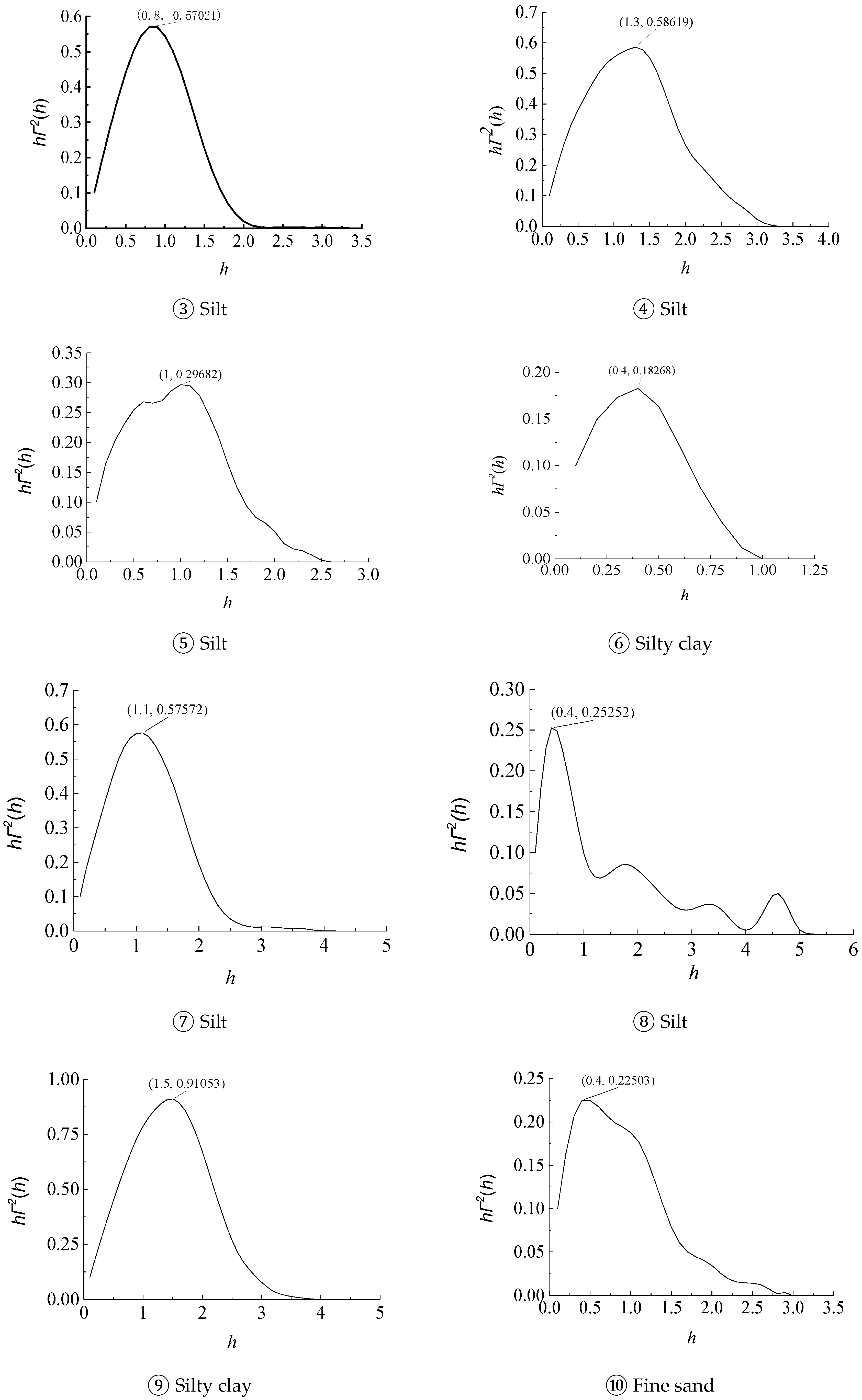
2.2. Calculation Method of Correlation Distance

Vanmarcke proposed the concept of correlation distance, which means there is a strong correlation between the physical and mechanical properties of each point within this distance range, and the properties of any two points beyond this range are not correlated with each other [20].

Many methods are available to calculate correlation distance [21,22,23]. The method of spatial average [24] is used in this paper. Assuming that there is a one-dimensional continuous stationary random field x(z), with a mean value of μ and a variance of σ, the local average random field within [z, z + h] is as follows:

$$x_h(z)=\frac{1}{h}{\displaystyle {\int }_z^{z+h}x(z)dz},$$

(1)

where h is the local average length.

The mean and variance of the local average random field are represented by Equations (2) and (3), respectively:

$$E[x_h(z)]=E[\frac{1}{h}{\displaystyle {\int }_z^{z+h}x(z)dz}]=\frac{1}{h}{\displaystyle {\int }_z^{z+h}E[x(z)]dz=\mu }$$

(2)

$$Var[x_h(z)]={\Gamma }^2(h)\cdot {\sigma }^2,$$

(3)

where Var[x_h(z)] is the spatial mean-variance of soil parameter, σ² is the point variance of soil parameter, h is the average spatial range, and Γ²(h) is the reduction function of variance.

Equation (2) presents that the mean value of the local average random field x_h(z) is the same as that of the original random field x(z). Equation (3) shows that the spatial mean-variance under space mean conditions is reduced by a certain degree based on the point variance.

The correlation distance δ can be expressed by [25]:

$$\delta =\underset{h\to \infty }{\lim }h{\Gamma }^2(h)$$

(4)

In practice, limited by foundation layer thickness, h cannot be infinite within a limited range, so when h is relatively large, it is approximately considered that

$$\delta =h{\Gamma }^2(h),$$

(5)

where Γ²(h) has the following property [26]:

$${\Gamma }^2(h)=\{\begin{array}{l}1, h<\delta \hfill \\ \frac{\delta }{h}, h\ge \delta \hfill \end{array}$$

(6)

The steps to calculate the correlation distance are as follows:

(1)

Select an average spatial range h = kh₀, where k is a positive integer and h₀ is the sampling spacing;

(2)

Take k = 1, 2, 3, …, in sequence and calculate the mean value of adjacent k + 1 points to form a spatial average random field x_h(z);

(3)

Calculate the point variance σ² and the spatial mean-variance Var[x_h(z)];

(4)

Calculate the variance reduction function Γ²(h) = Var[x_h(z)]/σ² by Equation (3);

(5)

Calculate the value of hΓ²(h) and draw the hΓ²(h)~h curve;

(6)

Find the value of hΓ²(h) that tends to converge smoothly from the hΓ²(h)~h curve and take it as the desired correlation distance δ.

2.3. Failure Probability of Pile Foundation

When designing a pile foundation, the standard value of the vertical ultimate bearing capacity of a single pile is as follows:

$$Q_{uk}=u{\displaystyle \sum q_{sik}{l}_i+q_{pk}{A}_p},$$

(7)

where Q_uk is the standard value of vertical ultimate bearing capacity of the single pile, q_sik is the standard value of ultimate lateral resistance of the i-th layer of soil at the pile side, q_pk is the standard value of ultimate tip resistance, l_i is the thickness of the i-th layer of soil around the pile, u is the perimeter of the pile, and A_p is the area of the pile tip.

The ultimate lateral resistance and ultimate tip resistance of each layer of soil are usually determined by lateral friction resistance and cone tip resistance obtained from the double-bridge static cone penetration test, where one sample of data can be obtained every 10 cm [27].

Pile foundation failure probability means the probability that the design pile foundation bearing capacity is less than the top pile load. Failure probability is calculated by the Monte Carlo method [28,29]. In the Monte Carlo method, parameter estimation can be conducted on failure probability P by the occurrence rate of the Bernoulli sequence. Assuming that there is a random variable sequence X₁, X₂, …, X_n, where X_i = 0 or 1 (i.e., the pile foundation fails or does not fail in the ith test), and the sequence X₁, X₂, …, X_n constitutes a random sample of size n, then the maximum likelihood estimate of the failure probability P is expressed by Equation (8):

$$\hat{P}=\frac{1}{n}{\displaystyle \sum _{i=1}^n{X}_i}=\frac{m}{n}$$

(8)

where $\widehat{P}$ is the estimate of the failure probability, n is the sample space, and m is the number of samples with the standard value of vertical ultimate bearing capacity of a single pile less than the average vertical force on single pile top.

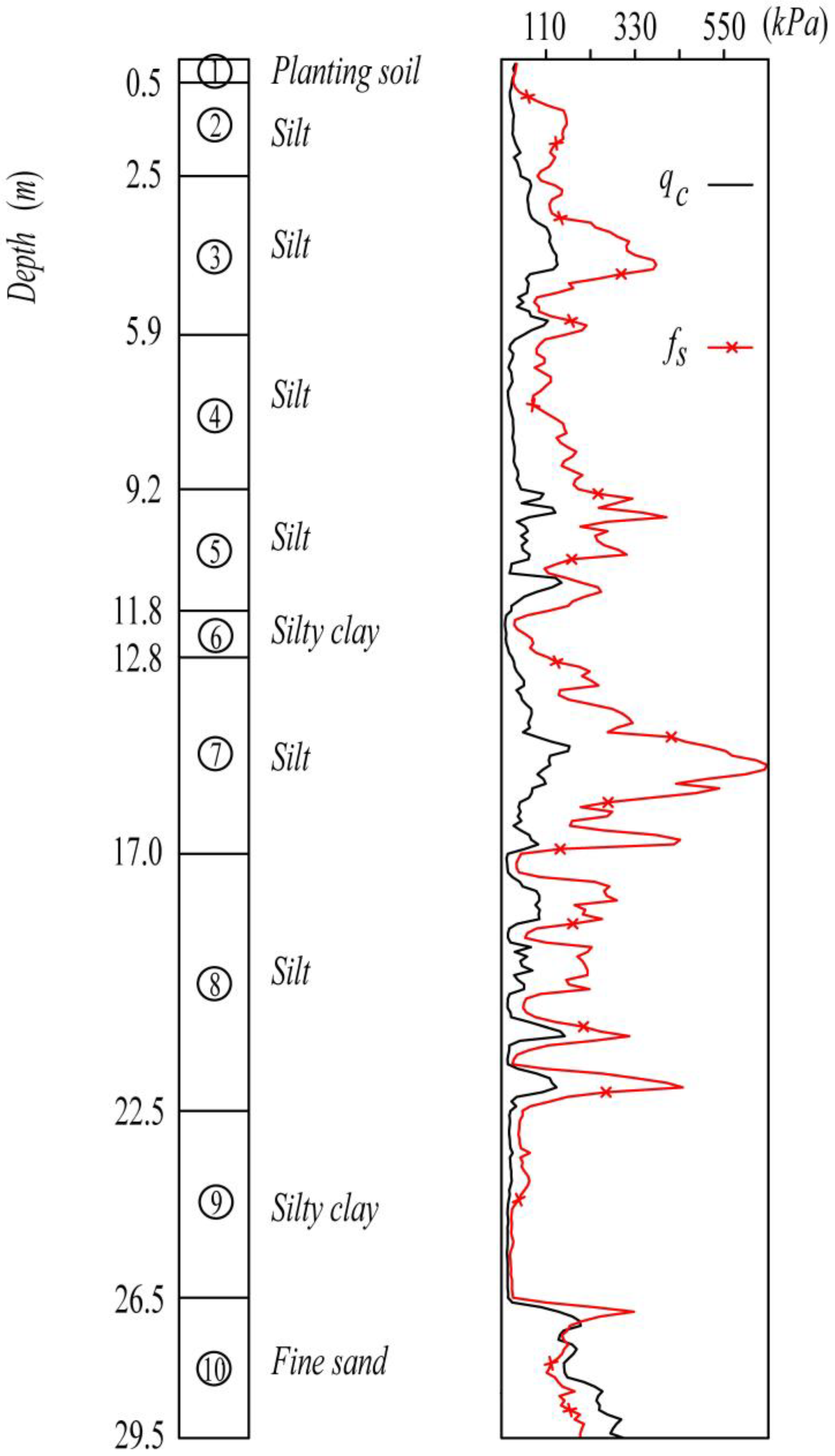
2.4. Static Cone Penetration Test Data

The experimental data of the single-hole foundation layer and double-bridge static cone penetration test of a project site in Dingxing County, Baoding City, are selected, as shown in Figure 1. Firstly, hypothesis testing is carried out on the lateral friction resistance and cone tip resistance measured in each layer of soil to obtain their respective probability distribution characteristics, and then the correlation distance of each layer of soil is calculated. Given the influence of the correlation distance, the probability distribution followed by lateral friction resistance and cone tip resistance in each layer of soil is obtained. In the two cases, random sampling is carried out according to their probability distribution characteristics to obtain random soil parameter samples, and then the pile foundation failure probability is calculated using the Monte Carlo method. The change in failure probability is compared and studied under the conditions of considering or not considering the correlation distance.

3. Results

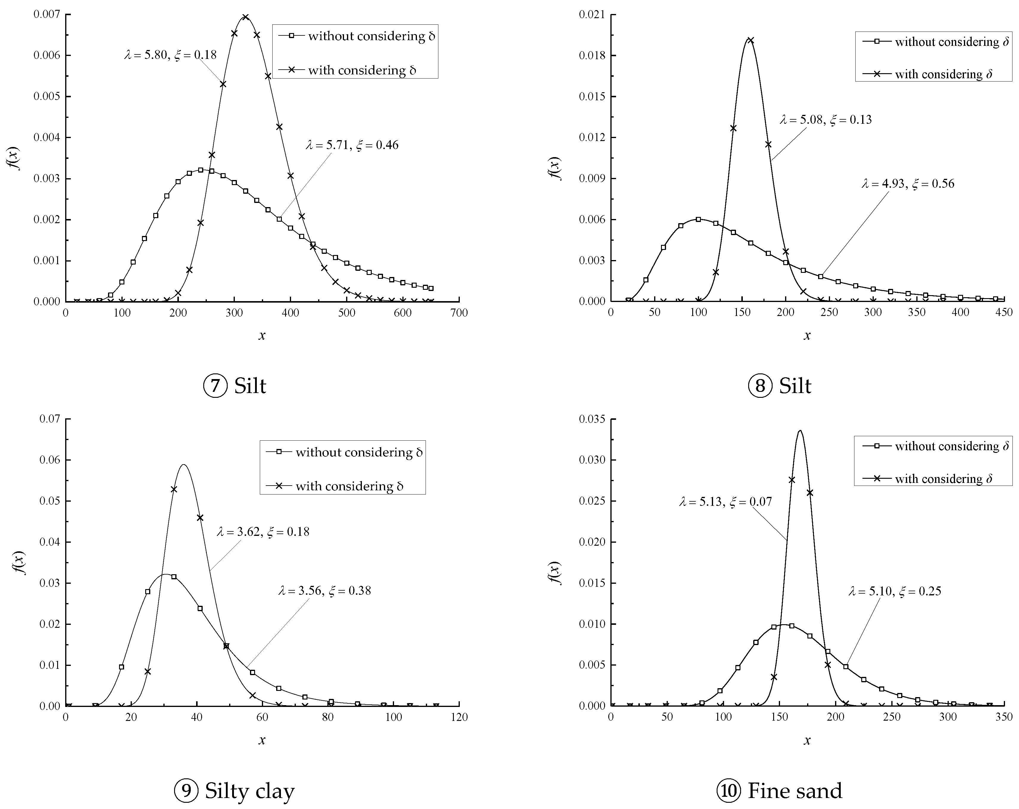
3.1. Distribution Characteristics of Each Layer of Soil Parameters without Considering the Influence of Correlation Distance

According to the static cone penetration test data, the sampling spacing h₀ = 10 cm, and the statistical parameters of sample data, such as lateral friction resistance and cone tip resistance of each layer of soil, are shown in

Table 1. Statistical parameters of sample data of each layer of soil from static cone penetration test.

Layer Name	Lateral Friction Resistance (kPa)		Cone Tip Resistance (kPa)
	Mean	Standard Deviation	Mean	Standard Deviation
① Planting soil	32.74	3.20	2.97	0.34
② Silt	118.98	37.51	3.19	0.84
③ Silt	199.87	91.60	8.55	2.94
④ Silt	130.32	37.33	2.79	0.79
⑤ Silt	227.57	72.71	6.89	3.77
⑥ Silty clay	64.79	24.54	1.33	0.51
⑦ Silt	334.35	161.57	7.11	3.43
⑧ Silt	161.77	98.89	5.26	3.87
⑨ Silty clay	37.87	14.81	1.80	0.36
⑩ Fine sand	169.55	43.54	19.76	6.16

.

A hypothesis testing is carried out on the distribution characteristics of sample data on lateral friction resistance and cone tip resistance of each layer of soil. All the results follow a logarithmic normal distribution (λ, ζ), and the parameters are shown in

Table 2. Parameters (following logarithmic normal distribution) of sample data of each soil layer from static cone penetration test.

Layer Name	Lateral Friction Resistance		Cone Tip Resistance
	λ	ζ	λ	ζ
① Planting soil	3.48	0.10	1.08	0.11
② Silt	4.73	0.31	1.13	0.26
③ Silt	5.20	0.44	2.09	0.33
④ Silt	4.83	0.28	0.99	0.28
⑤ Silt	5.38	0.31	1.80	0.51
⑥ Silty clay	4.10	0.37	0.21	0.37
⑦ Silt	5.71	0.46	1.86	0.46
⑧ Silt	4.93	0.56	1.44	0.66
⑨ Silty clay	3.56	0.3772	0.57	0.20
⑩ Fine sand	5.10	0.25	2.94	0.30

.

In the case of not considering the influence of correlation distance, the distribution characteristics of each layer of soil parameters refer to point distribution characteristics rather than the average spatial distribution characteristics of original data. The average spatial distribution characteristics of each layer of soil parameters are calculated below by considering the influence of correlation distance.

3.2. Average Spatial Characteristics of Each Layer of Soil Parameters Considering the Influence of the Correlation Distance

3.2.1. Calculation of the Correlation Distance

Based on the sample data of cone tip resistance q_c and lateral friction resistance f_s obtained from the static cone penetration test data, the correlation distances of lateral friction resistance and cone tip resistance of each soil layer in the foundation are calculated with the method of spatial average. The hΓ²(h)~h graphs for each parameter are shown in Figure 2 and Figure 3.

In Figure 2 and Figure 3, theoretically, hΓ²(h) increases with the increase in h and eventually tends to a stable convergence value according to Equation (4). However, during the actual calculation process, the soil layer thickness H cannot tend to infinity since the thickness H of each layer of soil is within a finite range. As the average spatial range h increases and gradually approaches the soil layer thickness H; the sample size used for calculating the spatial mean-variance gradually decreases, and hΓ²(h) tends to increase and then decrease, so the peak values of the curves are taken as the correlation distances. The calculation results of the correlation distance of each soil layer are shown in

Table 3. Calculation results of correlation distance of each foundation soil layer.

Layer Name	Layer Bottom Depth (m)	Layer Thickness (m)	Correlation Distance (m)
			Calculated by Lateral Friction Resistance	Calculated by Cone Tip Resistance
① Planting soil	0.5	0.5	0.14	0.1
② Silt	2.5	2	0.21	0.29
③ Silt	5.9	3.4	0.57	0.50
④ Silt	9.2	3.3	0.59	0.40
⑤ Silt	11.8	2.6	0.30	0.17
⑥ Silty clay	12.8	1	0.18	0.13
⑦ Silt	17	4.2	0.58	0.52
⑧ Silt	22.5	5.5	0.25	0.25
⑨ Silty clay	26.5	4	0.91	0.93
⑩ Fine sand	29.5	3	0.23	0.36

.

3.2.2. Average Spatial Distribution Characteristics of Each Layer of Soil Parameters

The average spatial distribution characteristics of parameters of each layer of soil are described by the spatial mean-variance. From Equations (3) and (6), given the influence of correlation distance, the spatial mean-variance of the parameters is expressed by the following:

$$Var[x_H(z)]={\sigma }^2{\Gamma }^2(H)={\sigma }^2\frac{\delta }{H},$$

(9)

where δ is the correlation distance, and H is the soil-layer thickness.

By Equation (9), point variance is converted to spatial mean-variance, but the mean is unchanged. The statistical parameters of sample data on lateral friction resistance and cone tip resistance of each layer are shown in

Table 4. Statistical parameters of sample data of each soil layer from static cone penetration test considering the influence of correlation distance.

Layer Name	Lateral Friction Resistance (kPa)		Cone Tip Resistance (kPa)
	Mean	Standard Deviation	Mean	Standard Deviation
① Planting soil	32.74	1.69	2.97	0.15
② Silt	118.98	12.20	3.19	0.32
③ Silt	199.87	37.51	8.55	1.12
④ Silt	130.32	15.73	2.79	0.27
⑤ Silt	227.57	24.57	6.90	0.96
⑥ Silty clay	64.79	10.49	1.33	0.18
⑦ Silt	334.35	59.82	7.11	1.21
⑧ Silt	161.77	21.19	5.26	0.82
⑨ Silty clay	37.87	7.07	1.80	0.17
⑩ Fine sand	169.55	11.93	19.76	2.12

and

Table 5. Parameters (following logarithmic normal distribution) of sample data of each soil layer from static cone penetration test considering the influence of correlation distance.

Layer Name	Lateral Friction Resistance		Cone Tip Resistance
	λ	ζ	λ	ζ
① Planting soil	3.49	0.05	1.09	0.05
② Silt	4.77	0.10	1.16	0.10
③ Silt	5.28	0.19	2.14	0.13
④ Silt	4.86	0.12	1.02	0.10
⑤ Silt	5.42	0.11	1.92	0.14
⑥ Silty clay	4.16	0.16	0.27	0.14
⑦ Silt	5.80	0.18	1.95	0.17
⑧ Silt	5.08	0.13	1.65	0.16
⑨ Silty clay	3.62	0.18	0.58	0.10
⑩ Fine sand	5.13	0.07	2.98	0.11

.

3.3. Failure Probability of Pile Foundation

The average vertical force on the single bored pile top is 6500 kN, the design pile diameter is 0.6 m, and three pile lengths of 21 m, 23 m, and 25 m are used for comparative analysis. Random sampling is carried out on lateral friction resistance and cone tip resistance of each soil layer according to their probability distribution characteristics with a sample space of 50,000. With the Monte Carlo method, the failure probability of pile foundation is calculated by considering and not considering correlation distance, respectively, and the results are shown in

Table 6. Failure probability calculation results.

Pile Diameter (m)	Pile Length (m)	Failure Probability (%)
		Not Considering Correlation Distance	Considering Correlation Distance
0.6	21	24.57	1.196
	23	16.662	0.058
	25	13.944	0.028

.

Table 6 shows that, with the same pile size, the failure probability calculated is significantly reduced considering the influence of correlation distance. In the calculation of pile foundation bearing capacity, the failure probability must be controlled within a certain range to ensure safety, and the influence of correlation distance should be considered to save project cost under the premise of ensuring a pile foundation safety.

4. Discussion

4.1. Influence of Correlation Distance on Parameter Distribution

In order to compare the influence of correlation distance on parameter distribution, the probability density curves considering and not considering correlation distance δ are drawn in the same coordinate system, as shown in Figure 4 and Figure 5.

From Figure 4 and Figure 5, it is obvious that the average spatial probability distributions of lateral friction resistance and cone tip resistance become less dispersed, and the data distribution becomes more concentrated when considering the influence of correlation distance. Not considering the influence of correlation distance means that the value of parameters of each point is a completely independent point distribution. Considering the influence of correlation distance indicates that soil parameters of two points with a distance within the correlation distance range are correlated with each other, and this correlation reduces the dispersion degree of the average spatial distribution of data.

4.2. Error Analysis

Errors in failure probability are probability errors of the estimate at a certain level of confidence. For a large sample size n, according to the central limit theorem, the failure probability estimate $\widehat{P}$ (sample mean of failure probability) approximately follows a normal distribution. By Equation (8), the mean value and standard deviation of $\widehat{P}$ are Equations (10) and (11), respectively.

$$E(\widehat{P})=E\left(\frac{1}{n}{\displaystyle \sum _{i=1}^n{X}_i}\right)=\frac{1}{n}{\displaystyle \sum _{i=1}^{n}E{X}_i}=1\times p+0\times (1-p)=p;$$

(10)

$$Var(\widehat{P})=\frac{1}{n^2}{\displaystyle \sum _{i=1}^{n}Var(X_i)}=\frac{1}{n^2}{\displaystyle \sum _{i=1}^n[E(X_i^2)-E^2(X_i)]}=\frac{p(1-p)}{n},$$

(11)

where the random sample X_i is 0 or 1, p is the failure probability, $\widehat{P}$ is the sample estimate of p, and n is the sample size.

Equation (10) indicates that $\widehat{P}$ is an unbiased estimate of p.

In Equation (11), the variance can be approximated as follows:

$$Var(\widehat{P})=\frac{\widehat{p}(1-\widehat{p})}{n}.$$

(12)

By setting the confidence coefficient (1 − α) to 0.95, then

$$P\left(|\frac{\widehat{p}-E(\widehat{p})}{Var(\widehat{p})}|\le Z_{\alpha /2}\right)=1-\alpha ,$$

(13)

where Z_α/2 is the α/2 upper quantile of the standard normal distribution Φ(x), Z_α/2 = Φ⁻¹(1 − α/2) = 1.96

The confidence interval for p with a confidence level of 1 − α is as follows:

$$\left(\widehat{p}-Z_{\alpha /2}\sqrt{\frac{\widehat{p}(1-\widehat{p})}{n}} , \widehat{p}+Z_{\alpha /2}\sqrt{\frac{\widehat{p}(1-\widehat{p})}{n}}\right).$$

(14)

In Section 3.3, the pile diameter is 0.6 m, the confidence intervals for failure probability of different pile lengths are shown in

Table 7. Confidence intervals of failure probability.

Pile Diameter (m)	Pile Length (m)	Confidence Interval
		Not Considering Correlation Distance	Considering Correlation Distance
0.6	21	(0.24193, 0.24947)	(0.01101, 0.01291)
	23	(0.16335, 0.16989)	(0.00037, 0.00079)
	25	(0.13640, 0.14248)	(0.00013, 0.00043)

, and the lengths of each confidence interval are shown in

Table 8. Confidence interval lengths.

Pile Diameter (m)	Pile Length (m)	Confidence Interval Length
		Not Considering Correlation Distance	Considering Correlation Distance
0.6	21	0.00755	0.00191
	23	0.00653	0.00042
	25	0.00607	0.00029

.

Table 7 and Table 8 show that, as the pile length increases, the shorter the confidence interval length, the higher the interval estimation accuracy. Compared with the case of not considering the influence of correlation distance, the shorter the length of the confidence interval obtained, the higher the accuracy of the interval estimation in the case of considering the influence of correlation distance.

4.3. Action Mechanism of Correlation Distance

Correlation distance reflects the relationship between microcosmic composition and macroscopic properties of soil [30]. On the microscale, the soil is a loose deposit mixture composed of soil particles, pore water, pore air, and other materials. Different causes determine different soil structures. Soil particle skeleton, pore water, and pore air have their respective laws of movement, which are different from each other, and there are interactions between them. Obvious interfaces exist between soil particles, pore water, and pore air, which can be analyzed separately. On the microscale, they manifest as a deterministic phenomenon, while micro interfaces cannot be distinguished on the macroscale, and their feature sizes are much larger than those on the microscale. Macro parameters or indicators of each point in the soil layer exhibit strong spatial variability [31], and equations established based on continuous media theory cannot be directly used. In order to describe macro systems, we must adopt averaging methods to establish a relationship between point characteristics on the microscale and average spatial characteristics within a certain thickness range on the macroscale and translate such extremely inhomogeneous micro medium into a macro-continuous medium.

In order to better describe this spatial variability on the macroscale, it is necessary to convert point variance to spatial mean-variance using the variance reduction function to reflect the spatial variability on a macroscale with average spatial characteristics. The variance reduction function depends on the correlation distance of parameters [32,33]. Correlation distances exist in soil layers with continuous deposition [34]. During the formation process, the environment of soil layers is not exactly the same. Even in the same layer, it takes a long time before a certain thickness of the soil is formed, so the environments formed at two points with a closer distance are relatively close to each other with similar physical and mechanical properties, showing a certain correlation. The farther the distance, the greater the difference and the weaker the correlation. Therefore, a boundary value (i.e., correlation distance) exists. Within the correlation distance, due to similar deposition environment, soil material composition, water content, density, and other properties are relatively similar, parameters exhibit strong correlation, and parameters beyond the correlation distance range can be considered to be uncorrelated with each other.

5. Conclusions

In this paper, the correlation distance of soil parameters is introduced into pile foundation reliability design. Static cone penetration test data of a project site are used to describe the average spatial characteristics of soil parameters with random field theory and calculate the failure probability of pile foundation to study the influence of correlation distance on pile foundation failure probability.

The existence of correlation distances in the soil layer indicates different deposition environments of soil during its formation process. The deposition environments at points with a closer distance are more similar, and the soil parameters have a certain correlation. Beyond the correlation distance, the deposition environments are relatively different from each other, and soil parameters can be considered to be uncorrelated from each other.

The complex composition and structure of soil allow soil parameters to exhibit strong spatial variability in a macrolayer, and the relationship between microscopic composition and macroscopic properties of soil is established by the spatial averaging method. In the pile foundation reliability design, a variance reduction function can be obtained by considering the influence of correlation distance of soil parameters and used to convert the point variance of original measurement data of soil parameters to their spatial mean-variance, which reduces the degree of dispersion of parameters and accurately reflects the spatial variability of parameters in soil layer on a macroscale, decreases the failure probability of pile foundation design, improves the accuracy of calculation results, and lowers project cost.

References

1. Khalid, U.; Rehman, Z.u.; Mujtaba, H.; Farooq, K. 3D response surface modeling based in-situ assessment of physico-mechanical characteristics of alluvial soils using dynamic cone penetrometer. Transp. Geotech. 2022, 36, 100781. [Google Scholar] [CrossRef]
2. Ijaz, Z.; Zhao, C.; Ijaz, N.; Rehman, Z.u.; Ijaz, A. Spatial mapping of geotechnical soil properties at multiple depths in Sialkot region, Pakistan. Environ. Earth Sci. 2021, 80, 787. [Google Scholar] [CrossRef]
3. Ijaz, Z.; Zhao, C.; Ijaz, N.; Rehman, Z.u.; Ijaz, A. Novel application of Google earth engine interpolation algorithm for the development of geotechnical soil maps: A case study of mega-district. Geocarto Int. 2022, 2138566. [Google Scholar] [CrossRef]
4. Huang, Y.; He, Z.; Yashima, A.; Chen, Z.; Li, C. Multi-objective optimization design of pile-anchor structures for slopes based on reliability theory considering the spatial variability of soil properties. Comput. Geotech. 2022, 147, 104751. [Google Scholar] [CrossRef]
5. Ravichandran, N.; Mahmoudabadi, V.; Shrestha, S. Analysis of the bearing capacity of shallow foundation in unsaturated soil using monte carlo simulation. Int. J. Geosci. 2017, 8, 1231–1250. [Google Scholar] [CrossRef] [Green Version]
6. Sedlacek, G.; Müller, C. The European standard family and its basis. J. Constr. Steel. Res. 2006, 62, 1047–1059. [Google Scholar] [CrossRef]
7. Burdekin, F.M. General principles of the use of safety factors in design and assessment. Eng. Fail. Anal. 2007, 14, 420–433. [Google Scholar] [CrossRef]
8. Zhang, X.-l.; Jiao, B.-h.; Hou, B.-w. Reliability analysis of horizontally loaded pile considering spatial variability of soil parameters. Soil Dyn. Earthq. Eng. 2021, 143, 106648. [Google Scholar] [CrossRef]
9. Cao, Z.; Wang, Y. Bayesian approach for probabilistic site characterization using cone penetration tests. J. Geotech. Geoenviron. Eng. 2013, 139, 267–276. [Google Scholar] [CrossRef]
10. Wang, Y.; Shu, S.; Wu, Y. Reliability analysis of soil liquefaction considering spatial variability of soil property. J. Earthq. Tsunami 2022, 16, 2250002. [Google Scholar] [CrossRef]
11. Qi, X.; Wang, H.; Chu, J.; Chiam, K. Effect of autocorrelation function model on spatial prediction of geological interfaces. Can. Geotech. J. 2022, 59, 583–600. [Google Scholar] [CrossRef]
12. Fei, S.; Tan, X.; Lin, X.; Xiao, Y.; Zha, F.; Xu, L. Evaluation of the scale of fluctuation based on variance reduction method. Eng. Geol. 2022, 308, 106804. [Google Scholar] [CrossRef]
13. Le, T.M.H.; Sánchez, M.; Gallipoli, D.; Wheeler, S. Probabilistic modelling of auto-correlation characteristics of heterogeneous slopes. Geomech. Geoengin. 2015, 10, 95–108. [Google Scholar] [CrossRef]
14. Oguz, E.A.; Huvaj, N.; Griffiths, D.V. Vertical spatial correlation length based on standard penetration tests. Mar. Geores. Geotechnol. 2019, 37, 45–56. [Google Scholar] [CrossRef]
15. Vessia, G.; Russo, S. Random field theory to interpret the spatial variability of lacustrine soils. Biosyst. Eng. 2018, 168, 4–13. [Google Scholar] [CrossRef]
16. Yang, Y.; Tang, H.; Wang, X. Failure probability analysis of corroded RC structures considering the effect of spatial variability. Mag. Concr. Res. 2023, 75, 163–175. [Google Scholar] [CrossRef]
17. Ching, J.; Phoon, K.-K.; Sung, S.-P. Worst case scale of fluctuation in basal heave analysis involving spatially variable clays. Struct. Saf. 2017, 68, 28–42. [Google Scholar] [CrossRef]
18. Luo, Z.; Kim, M.; Hwang, S. Effect of soil spatial variability on the structural reliability of a statically indeterminate frame. ASCE-ASME J. Risk. Uncertain. Eng. Syst. Part A-Civ. Eng. 2021, 7, 04020048. [Google Scholar] [CrossRef]
19. Lo, M.K.; Leung, Y.F.; Ku, T. Variability response function approach for foundation reliability. Probab. Eng. Eng. Mech. 2021, 64, 103129. [Google Scholar] [CrossRef]
20. Kawa, M.; Bagińska, I.; Wyjadłowski, M. Reliability analysis of sheet pile wall in spatially variable soil including CPTu test results. Arch. Civ. Mech. Eng. 2019, 19, 598–613. [Google Scholar] [CrossRef]
21. Wang, T.; Cao, J.; Pei, X.; Hong, Z.; Liu, Y.; Zhou, G. Research on spatial scale of fluctuation for the uncertain thermal parameters of artificially frozen soil. Sustainability 2022, 14, 16521. [Google Scholar] [CrossRef]
22. Pieczyńska-Kozłowska, J.M. Comparison between two methods for estimating the vertical scale of fluctuation for modeling random geotechnical problems. Stud. Geotech. Mech. 2015, 37, 95–103. [Google Scholar] [CrossRef] [Green Version]
23. Cami, B.; Javankhoshdel, S.; Phoon, K.-K.; Ching, J. Scale of fluctuation for spatially varying soils: Estimation methods and values. ASCE-ASME J. Risk. Uncertain. Eng. Syst. Part A-Civ. Eng. 2020, 6, 03120002. [Google Scholar] [CrossRef]
24. Yan, S.; Guo, L. Calculation of scale of fluctuation and variance reduction function. Trans. Tianjin Univ. 2015, 21, 41–49. [Google Scholar] [CrossRef]
25. Christodoulou, P.; Pantelidis, L.; Gravanis, E. A comparative assessment of the methods-of-moments for estimating the correlation length of one-dimensional random fields. Arch. Comput. Method Eng. 2020, 28, 1163–1181. [Google Scholar] [CrossRef]
26. Metya, S.; Bhattacharya, G. Reliability analysis of earth slopes considering spatial variability. Geotech. Geol. Eng. 2016, 34, 103–123. [Google Scholar] [CrossRef]
27. Ebrahimian, B.; Movahed, V. Application of an evolutionary-based approach in evaluating pile bearing capacity using CPT results. Ships Offshore Struct. 2016, 12, 937–953. [Google Scholar] [CrossRef]
28. Luo, N.; Luo, Z. Risk assessment of footings on slopes in spatially variable soils considering random field rotation. ASCE-ASME J. Risk. Uncertain. Eng. Syst. Part A-Civ. Eng. 2022, 8, 04022028. [Google Scholar] [CrossRef]
29. Homaei, F.; Najafzadeh, M. Failure analysis of scouring at pile groups exposed to steady-state flow: On the assessment of reliability-based probabilistic methodology. Ocean Eng. 2022, 266, 112707. [Google Scholar] [CrossRef]
30. Feng, D. Modal analysis of beam structures with random field models at multiple scales. Adv. Civ. Eng. 2021, 2021, 8847771. [Google Scholar] [CrossRef]
31. Cai, G.; Lin, J.; Liu, S.; Puppala, A.J. Characterization of spatial variability of CPTU data in a liquefaction site improved by vibro-compaction method. KSCE J. Civ. Eng. 2016, 21, 209–219. [Google Scholar] [CrossRef]
32. Onyejekwe, S.; Kang, X.; Ge, L. Evaluation of the scale of fluctuation of geotechnical parameters by autocorrelation function and semivariogram function. Eng. Geol. 2016, 214, 43–49. [Google Scholar] [CrossRef]
33. Liu, Y.; He, L.Q.; Jiang, Y.J.; Sun, M.M.; Chen, E.J.; Lee, F.H. Effect of in-situ water content variation on the spatial variation of strength of deep cement-mixed clay. Geotechnique 2019, 69, 391–405. [Google Scholar] [CrossRef] [Green Version]
34. Liu, Z.; Marit Wist Amdal, Å.; L’Heureux, J.-S.; Lacasse, S.; Nadim, F.; Xie, X. Spatial variability of medium dense sand deposit. AIMS Geosci. 2020, 6, 6–30. [Google Scholar] [CrossRef]
Figure 1. Static cone penetration curve (lateral friction resistance fs and cone tip resistance qc).
Sustainability 15 04298 g001
Figure 2. hΓ2(h)~h graph for lateral friction resistance of each soil layer.
Sustainability 15 04298 g002aSustainability 15 04298 g002b
Figure 3. hΓ2(h)~h graph for cone tip resistance of each soil layer.
Sustainability 15 04298 g003aSustainability 15 04298 g003b
Figure 4. Probability distribution of lateral friction resistance.
Sustainability 15 04298 g004aSustainability 15 04298 g004b
Figure 5. Probability distribution of cone tip resistance.
Sustainability 15 04298 g005aSustainability 15 04298 g005b