Adjustment of Measurement Error Effects on Dispersion Control Chart with Distribution-Free Quality Variable

Abstract

In industrial processes, control charts are useful tools to monitor the quality of products and detect possibly out-of-control processes. While many types of control charts have been available for data analysts, they were developed by assuming that the variables are precisely measured. In applications, however, measurement error is ubiquitous when data are falsely recorded by investigators or imprecisely collected by unadjusted machines. Even though the impacts of measurement error for different types of control charts have been explored, error-corrected control charts are still unavailable. In this study, we propose a new dispersion control chart with error correction to fill out this research gap. Our key idea is to convert the observed distribution-free process variables into a flexible sign statistic, and then adopt a function to adjust the measurement error effects on the sign statistic. Finally, we develop an exponentially weight-moving average dispersion control chart with measurement error correction based on the corrected sign statistic. The proposed error-corrected dispersion control chart not only eliminates measurement error effects, but also provides more reliable control limits for monitoring process dispersion. Throughout the numerical examination, we find that the proposed error-corrected dispersion control chart is effective in handling moderate and large levels of measurement error and shows good out-of-control detection performance. Finally, the proposed error-corrected dispersion control chart is implemented in the semiconductor data.

1. Introduction

Statistical process control (SPC) is a useful tool to maintain the quality of the product and detect possibly out-of-control (OC) processes. Many methods have been developed and widely applied since the work of Shewhart [1], including the $\overline{X}$ chart used to monitor the mean of the process, and $R$ or $S$ chart adopted to monitor the dispersion of the process. However, they are not sensitive to detecting small shifts. To remedy this, Robert [2] proposed an exponentially weighted moving average (EWMA) chart, which improves out-of-control detection performance against the Shewhart control chart for the mean and dispersion with small shifts.

Another critical concern of Shewhart charts is the requirement of the normally distributed data, which is usually violated in applications. To improve this shortcoming, several distribution-free methods have been explored. To name a few, Amin et al. [3] proposed the sign chart based on sign-test statistics to control process center and variability. Bakir [4,5] proposed the Shewhart type that is based on the sign test or signed ranks of grouped observations to monitor a process center. These charts do not require the distribution to be symmetric, and they are applicable in various situations. Yang et al. [6] proposed the nonparametric EWMA sign chart to monitor the process target. Yang et al. [7] proposed the nonparametric EWMA sign chart to monitor the process mean. Chowdhury et al. [8] proposed the Shewhart–Cucconi (SC) chart to monitor a process location and scale. Although these methods address the issue of requiring normality assumptions, they may not necessarily perform better when the sample size is large. Yang and Arnold [9,10] developed a distribution-free dispersion control chart, whose monitoring statistic will not be influenced by out-of-control mean. Tang et al. [11] proposed an AEWMA median chart with known or estimated parameters to monitor the mean value. Riaz et al. [12] proposed an NPSNDH control chart based on sign test statistics to monitor process location. These charts solve the issue of distributional assumptions but, unfortunately, cannot be directly applied in more general situations that involve measurement errors.

Those existing methods are under the assumption that data are precisely measured. In applications, however, measurement error is ubiquitous when data are falsely recorded by the investigators or imprecisely collected by unadjusted machines. This feature may incur the wrong conclusion or induce an incorrect control chart. In the past literature, measurement error effects have been investigated based on several types of control charts. For example, for location and scale processes, Mittag and Stemann [13] proved stochastic measurement error has considerable effects on Shewhart $\overline{X}-S$ control charts. Linna and Woodall [14] examined measurement error effects on Shewhart $\overline{X}$ and $S^2$ charts by using covariable models and linearly increasing variance models. Stemann and Weihs [15] compared the ability of the EWMA-$\overline{X}-S$ chart and the Shewhart $\overline{X}-S$ chart with measurement error and found that the EWMA-$\overline{X}-S$ chart is superior. To monitor the mean process with measurement error, Maravelakis et al. [16] examined the effect of measurement error on EWMA-$\overline{X}$ charts for mean by using a covariable model, multiple measurements, and a linearly increasing variance model. Abbas et al. [17] proposed EWMA control charts using auxiliary variables in the form of regression estimates to monitor process means. Daryabari et al. [18] examined measurement error effects on the Maximum Exponentially Weighted Moving Average and Mean Squared deviation (MAX EWMAMS) control chart, which can monitor mean and variance processes; Noor-ul-Amin et al. [19] examined measurement error effects with an auxiliary variable for EWMA-Z control charts by using a covariable model, multiple measurements, and a linearly increasing variance model. Asif et al. [20] described measurement error effects on the hybrid exponentially weighted moving average (HEWMA) control chart by using a covariable model, multiple measurements, and a linearly increasing variance model. Huwang and Hung [21] examined the effect of measurement error on the sample generalized variance chart and the likelihood ratio test chart for monitoring multivariate process variability. Nojavan et al. [22] examined the effect of measurement error on Mann–Whitney and signed-rank charts for monitoring the process center when the distribution is unknown. While these methods discuss the effect of different measurement error models on control charts, they do not provide suitable strategies to correct for measurement error effects.

In addition to continuous random variables, $p$ control charts subject to error-prone binary random variables have also been explored. For example, Case [23] showed that inspection error rates affected the OC curve of a $p$ control chart and proposed the compensating $p$ chart to make the actual OC curve into the proximity of the desired OC curve. Lu et al. [24] examined the effect of inspection error on run-length control charts and presented the adjusted control limits for the run-length charts to partially compensate for the shifts of the average number inspected (ANI) curves with inspection error. Shu and Wu [25] used fuzzy set theory to construct a fuzzy-$p$ control chart and monitor the imprecise fraction of nonconforming items. Daryabari [26] examined the performance of the Bernoulli CUSUM chart in the presence of measurement error. Chen and Yang [27] proposed an error-corrected EWMA $p$ control chart to monitor the changes in defection rate. These methods examine or correct for the impacts of measurement error on control charts, providing us with a good direction for addressing the issue of measurement error.

Although some methods have been developed to reduce the effect of measurement error, such as Case [23], Shu and Wu [25], and Chen and Yang [27], few approaches are available to correct for measurement error effects when monitoring continuous random variables. Most methods assume the true quality characteristics and the measurement error are normal distributions. On the contrary, a few studies only discuss the effect of measurement error on process dispersion. Therefore, we propose a new approach to correct measurement error effects for monitoring process dispersion. Specifically, we apply the dispersion statistic of the sign chart proposed by Yang and Arnold [9,10] to transform continuous random variables into discrete ones. After that, we develop an error-corrected EWMA variance control chart by adopting a corrected proportion (e.g., Chen and Yang [27]). Our contribution is to propose an error-eliminated and distribution-free dispersion control chart, which provides reliable control limits and effectively detects out-of-control processes.

The remainder is organized as follows. In Section 2, following Yang and Arnold [10], we introduce the general framework of the EWMA variance chart and discuss measurement error effects for the EWMA variance chart. We also propose a valid approach to correct measurement error effects. To assess the performance of detecting out-of-control process dispersion, we examine the out-of-control average run length ($AR{L}_1$) and compare the performance of the EWMA variance with/without measurement error correction in Section 3. In Section 4, we examine the robustness of the proposed chart by considering different distributions of true observation and various levels of measurement error. In Section 5, we apply the proposed variance control chart to analyze the SECOM data set from the UCI Machine Learning Repository [28] and compare the detection performance with the EWMA variance chart with measurement error. A summary is given in Section 5.

2. Using the Error-Corrected EWMA Variance Chart to Monitor Process Dispersion

2.1. Design of the EWMA Variance Chart

Yang and Arnold [9,10] proposed a dispersion monitoring statistic whose variance will not be influenced by the out-of-control mean and integrated it with the sign test method to construct the distribution-free EWMA dispersion control charts. We adopted the general framework of the EWMA dispersion control chart in Yang and Arnold [9,10], and described it as follows.

Let $n$ be the sample size, and let $t$ denote the number of sampling periods. For the $t^{th}$ sampling period and the $j^{th}$ observation with $j=1,\cdots ,n$ and $t=1,\cdots ,\infty$, let $X_{t,j}$ be continuous random samples coming from an in-control continuous process $X_0$ with unknown distribution and variance ${\sigma }^2$.

To monitor the process variance under the unknown distribution, we can use the sign method to convert the continuous variable to a binary variable. Specifically, under the in-control process, define

$$Y_{t, j^{{}^{\prime }}}=\frac{{\left(X_{t, 2 j^{{}^{\prime }}}-X_{t,2 j^{{}^{\prime }}-1}\right)}^2}{2}$$

(1)

for a fixed $t$ and $j^{{}^{\prime }}=1,2,\cdots ,0.5n$. Based on the transformation (1), we denote $Y_0$ as the random variable of the in-control process, then we obtain $E\left(Y_0\right)={\sigma }^2$. We can see that the statistic $Y_0$ is an unbiased estimator of ${\sigma }^2$, and it will not be influenced by the mean of $X_{t, 2 j^{{}^{\prime }}}$.

Moreover, by (1), define an indicator function

$$I_{t,j^{{}^{\prime }}}=\{\begin{array}{c}1, if Y_{t,j^{{}^{\prime }}}>{\sigma }^2\\ 0, \mathit{otherwise}\end{array} \mathrm{for} \mathrm{fixed} t \mathrm{and} j^{{}^{\prime }}=1,2,\cdots ,0.5n.$$

(2)

Denote $V_t$ as the sum of indicators of function at the $t^{th}$ sampling period, i.e.,

$$V_t={\sum }_{j^{{}^{\prime }}=1}^{0.5n}{I}_{t,j^{{}^{\prime }}}~Bin\left(0.5n,p_0\right) \mathrm{for} t = 1,\cdots ,\infty ,$$

(3)

where $p_0\triangleq P\left(Y_0>{\sigma }^2\right)$ for the in-control process.

From (3), let

$$P_t=\frac{V_t}{0.5n} \mathrm{for} t = 1,\cdots ,\infty ,$$

(4)

To monitor the variance process, we can construct an EWMA variance chart based on (4), and the EWMA statistic at $t$ time is defined as

$$EWM{A}_{P_t}=\lambda P_t+\left(1-\lambda \right)EWM{A}_{P_{t-1}}$$

(5)

for $t=1, 2,\cdots ,\infty$, where $\lambda$ is a smoothing parameter, and $\lambda \in \left(0,1\right]$.

We let the starting EWMA charting statistic, $EWM{A}_{P_0}$, $t=0$, be the mean of $P_t$, i.e., $EWM{A}_{P_0}=p_0$. The mean and the variance of $EWM{A}_{P_t}$ are, respectively, derived as

$$E\left(EWM{A}_{P_t}\right)=p_0$$

and

$$Var\left(EWM{A}_{P_t}\right)=\frac{p_0\left(1-p_0\right)\lambda \left[1-{\left(1-\lambda \right)}^{2t}\right]}{n\left(2-\lambda \right)}.$$

Assume that there is an upward or downward out-of-control process dispersion; hence, two one-sided EWMA variance charts are considered. The control limits ($\left(UC{L}_1,LC{L}_1\right)$ and $\left(UC{L}_2,LC{L}_2\right)$) of the two one-sided EWMA variance charts are, respectively, as follows.

$$\begin{array}{c}UC{L}_1=p_0+L_1\sqrt{\frac{p_0\left(1-p_0\right)\lambda \left[1-{\left(1-\lambda \right)}^{2t}\right]}{n\left(2-\lambda \right)}},\hfill \\ LC{L}_1=-\infty ,\hfill \end{array}$$

(6)

and

$$\begin{array}{c}UC{L}_2=\infty ,\hfill \\ LC{L}_2 = p_0-L_2\sqrt{\frac{p_0\left(1-p_0\right)\lambda \left[1-{\left(1-\lambda \right)}^{2t}\right]}{n\left(2-\lambda \right)}},\hfill \end{array}$$

(7)

where $L_1$ and $L_2$ are determined to satisfy the preset in-control average run length ($AR{L}_0$).

To calculate the $L_1$ and $L_2$, we first define run length ($RL$), which is the first number of points that will point beyond the control limits. The average run length ($ARL$) is the mean of $RL$. With given the $ARL$, one can adopt a numerical algorithm summarized in Algorithm 1 to determine $L_1$ and $L_2$.

To assess the performance of process monitoring, we primarily examine the $AR{L}_0$, in-control median run length ($MRL$), and in-control standard deviation of run length ($SDRL$), denoted as $MR{L}_0$ and $SDR{L}_0$. We employ Monte Carlo simulation to compute $AR{L}_0$, $MR{L}_0$, $SDR{L}_0$, and let ${\widehat{ARL}}_0$, ${\widehat{MRL}}_0$, ${\widehat{SDRL}}_0$ denote resulting values. The $AR{L}_0$ is usually set as $370.4$ and $200$. In this study, we set $AR{L}_0=370.4$. In principle, larger values of $SDR{L}_0$ indicate we need more $RL$ to ensure the ${\widehat{ARL}}_0$ is precise enough and close to prespecified $AR{L}_0$. Generally, the distribution of $RL$ is skewed; hence, $MRL$ is a robust version of the $ARL$, and we can use $MR{L}_0$ to measure the central tendency.

We further adopt the algorithm in Appendix A to run the simulation and assess the control limits of the EWMA variance chart ($UC{L}_1$ and $LC{L}_2$), considering $p_0=0.1\left(0.05\right)0.45$, $AR{L}_0=370.4$ and $\lambda =0.05$. Numerical results are placed in Table 1, where some values of $L_2$ do not exist since $LC{L}_2$ may not converge under small $p_0$ and $n$. We find that the widths of the two control charts become narrower when $p_0$ or the sample size $n$ increases.

Table 1. The $L_1$ and $L_2$ of the two one-sided EWMA variance charts with $AR{L}_0\approx 370.4$ and $\lambda =0.05$ for various $0.5n$.

$0.5\mathit{n}$	${\mathit{p}}_0$	0.1	0.15	0.2	0.25	0.3	0.35	0.4	0.45	$0.5\mathit{n}$	${\mathit{p}}_0$	0.1	0.15	0.2	0.25	0.3	0.35	0.4	0.45
1	$L_1$	2.613	2.487	2.415	2.377	2.317	2.269	2.243	2.208	5	$L_1$	2.346	2.291	2.284	2.260	2.236	2.215	2.206	2.201
	$UC{L}_1$	0.226	0.292	0.355	0.415	0.470	0.523	0.576	0.626		$UC{L}_1$	0.150	0.209	0.265	0.320	0.373	0.426	0.477	0.528
	${\widehat{ARL}}_0$	369.420	369.675	370.404	370.474	369.596	370.991	370.363	370.821		${\widehat{ARL}}_0$	370.226	370.838	370.620	371.295	369.494	370.277	369.487	370.062
	${\widehat{MRL}}_0$	235.000	239.000	254.000	246.000	251.000	254.000	252.000	250.000		${\widehat{MRL}}_0$	243.000	251.000	248.000	246.000	244.500	251.000	248.000	249.000
	${\widehat{SDRL}}_0$	412.550	403.998	389.989	398.119	383.980	395.516	387.791	381.086		${\widehat{SDRL}}_0$	396.058	396.092	394.681	393.823	393.857	384.115	387.144	386.935
	$L_2$	-	-	-	1.950	2.005	2.058	2.099	2.141		$L_2$	1.983	2.035	2.067	2.079	2.100	2.132	2.144	2.161
	$LC{L}_2$	-	-	-	0.115	0.153	0.193	0.235	0.279		$LC{L}_2$	0.057	0.098	0.141	0.186	0.231	0.277	0.325	0.373
	${\widehat{ARL}}_0$	-	-	-	370.255	369.771	370.948	370.163	370.738		${\widehat{ARL}}_0$	369.530	369.474	370.561	369.588	370.623	369.479	371.332	369.727
	${\widehat{MRL}}_0$	-	-	-	257.000	251.500	256.000	249.000	251.000		${\widehat{MRL}}_0$	254.000	253.000	249.000	254.500	254.000	255.000	253.000	251.000
	${\widehat{SDRL}}_0$	-	-	-	372.858	377.576	375.234	379.337	378.038		${\widehat{SDRL}}_0$	371.532	377.845	376.666	376.126	382.532	381.160	386.535	384.101
2	$L_1$	2.476	2.394	2.357	2.334	2.257	2.226	2.188	2.206	10	$L_1$	2.298	2.267	2.260	2.225	2.213	2.205	2.200	2.188
	$UC{L}_1$	0.184	0.247	0.307	0.364	0.417	0.470	0.521	0.574		$UC{L}_1$	0.135	0.191	0.246	0.299	0.351	0.403	0.455	0.505
	${\widehat{ARL}}_0$	369.991	370.072	370.145	371.292	369.780	370.679	370.073	369.673		${\widehat{ARL}}_0$	370.617	370.869	371.290	370.122	370.993	370.213	370.239	370.927
	${\widehat{MRL}}_0$	243.000	245.000	243.000	237.000	253.000	247.000	246.000	245.000		${\widehat{MRL}}_0$	249.000	248.000	242.000	245.500	251.000	245.000	247.000	248.000
	${\widehat{SDRL}}_0$	402.733	398.480	402.038	418.830	383.062	390.341	394.619	391.579		${\widehat{SDRL}}_0$	388.704	394.289	400.223	392.066	382.948	394.178	396.160	402.867
	$L_2$	-	1.929	1.994	2.038	2.077	2.096	2.130	2.160		$L_2$	2.042	2.069	2.104	2.107	2.127	2.141	2.156	2.166
	$LC{L}_2$	-	0.072	0.110	0.150	0.192	0.237	0.282	0.328		$LC{L}_2$	0.069	0.113	0.157	0.204	0.251	0.298	0.347	0.395
	${\widehat{ARL}}_0$	-	369.795	370.292	369.624	371.360	369.707	370.198	369.799		${\widehat{ARL}}_0$	369.625	370.507	369.704	370.791	369.860	370.264	370.703	370.200
	${\widehat{MRL}}_0$	-	254.000	253.000	255.000	258.000	257.500	252.500	248.000		${\widehat{MRL}}_0$	257.000	254.000	250.000	253.000	253.000	255.000	253.000	254.000
	${\widehat{SDRL}}_0$	-	366.828	374.765	372.839	370.337	375.441	382.434	387.196		${\widehat{SDRL}}_0$	372.408	381.782	384.500	383.480	384.760	384.321	386.322	383.801
3	$L_1$	2.413	2.379	2.297	2.260	2.258	2.247	2.211	2.191	15	$L_1$	2.278	2.256	2.244	2.225	2.207	2.199	2.193	2.188
	$UC{L}_1$	0.167	0.229	0.285	0.340	0.396	0.449	0.500	0.551		$UC{L}_1$	0.128	0.183	0.237	0.290	0.342	0.393	0.444	0.495
	${\widehat{ARL}}_0$	370.040	370.235	370.268	370.666	370.045	371.308	370.140	369.708		${\widehat{ARL}}_0$	369.836	370.626	371.081	370.033	370.043	369.848	369.514	370.129
	${\widehat{MRL}}_0$	241.000	239.000	249.000	250.000	247.000	247.000	247.000	252.000		${\widehat{MRL}}_0$	248.000	241.000	253.000	247.000	249.000	245.000	252.000	248.000
	${\widehat{SDRL}}_0$	410.201	419.206	388.305	393.618	394.359	393.442	392.217	382.364		${\widehat{SDRL}}_0$	393.615	397.972	393.131	387.314	393.538	398.568	387.483	390.523
	$L_2$	1.903	1.987	2.039	2.070	2.096	2.119	2.128	2.142		$L_2$	2.060	2.099	2.111	2.130	2.140	2.151	2.160	2.164
	$LC{L}_2$	0.047	0.084	0.125	0.167	0.211	0.257	0.304	0.351		$LC{L}_2$	0.074	0.119	0.165	0.212	0.259	0.308	0.356	0.405
	${\widehat{ARL}}_0$	370.466	369.623	370.715	370.609	369.563	370.330	371.315	369.499		${\widehat{ARL}}_0$	369.405	369.883	369.477	370.392	370.871	370.095	370.566	369.836
	${\widehat{MRL}}_0$	259.000	256.000	251.000	252.000	251.000	249.000	255.000	251.000		${\widehat{MRL}}_0$	252.000	254.000	248.000	253.000	253.000	254.000	246.000	248.000
	${\widehat{SDRL}}_0$	365.805	373.471	378.276	378.575	380.180	386.924	381.078	380.577		${\widehat{SDRL}}_0$	380.427	378.320	383.260	388.381	381.714	386.921	387.769	390.595
4	$L_1$	2.397	2.323	2.283	2.283	2.238	2.231	2.207	2.201	20	$L_1$	2.261	2.244	2.234	2.213	2.209	2.199	2.191	2.185
	$UC{L}_1$	0.158	0.216	0.273	0.329	0.382	0.435	0.487	0.538		$UC{L}_1$	0.124	0.179	0.232	0.284	0.336	0.388	0.438	0.489
	${\widehat{ARL}}_0$	371.321	370.706	370.574	370.321	370.476	370.325	369.423	369.420		${\widehat{ARL}}_0$	371.387	369.791	369.980	369.997	369.858	370.371	369.666	371.246
	${\widehat{MRL}}_0$	242.000	247.000	244.000	246.000	254.000	246.000	250.000	249.000		${\widehat{MRL}}_0$	251.000	242.000	244.000	250.000	248.000	247.000	245.000	258.000
	${\widehat{SDRL}}_0$	407.499	395.937	401.268	404.545	384.346	397.136	390.870	395.529		${\widehat{SDRL}}_0$	391.442	400.053	394.166	386.493	394.756	394.480	399.119	384.545
	$L_2$	1.953	2.020	2.054	2.083	2.098	2.108	2.146	2.155		$L_2$	2.078	2.106	2.123	2.132	2.143	2.154	2.160	2.171
	$LC{L}_2$	0.053	0.092	0.134	0.178	0.223	0.270	0.316	0.364		$LC{L}_2$	0.078	0.123	0.170	0.217	0.265	0.313	0.362	0.411
	${\widehat{ARL}}_0$	370.922	371.149	370.306	370.275	369.723	371.398	371.107	370.641		${\widehat{ARL}}_0$	369.451	371.155	369.614	371.117	369.757	370.893	370.751	371.368
	${\widehat{MRL}}_0$	259.000	250.000	248.500	255.000	249.000	250.000	251.000	248.000		${\widehat{MRL}}_0$	253.000	250.000	253.000	247.000	248.000	252.000	250.500	247.000
	${\widehat{SDRL}}_0$	371.410	379.139	380.352	373.165	382.879	383.836	392.866	380.232		${\widehat{SDRL}}_0$	385.076	382.976	385.942	388.587	395.258	393.000	389.536	392.700

2.2. The EWMA Variance Chart with Measurement Error

In applications, instead of observing $X_{t,j}$, we usually collect the surrogate version of $X_{t,j}$, denoted as $X_{t,j}^{*}$. To characterize $X_{t,j}$ and $X_{t,j}^{*}$, we adopt the classical measurement error model

$$X_{t,j}^{*}=X_{t,j}+{\epsilon }_{t,j},$$

(8)

where ${\epsilon }_{t,j}$ is a random sample with $E\left({\epsilon }_{t,j}\right) = 0$ and $Var\left({\epsilon }_{t,j}\right)={\delta }_2^2{\sigma }^2$ for some positive constant ${\delta }_2$. We assume that ${\epsilon }_{t,j}$ is independent of $X_{t,j}$. By (8), it is straightforward that the variance of $X_{t,j}^{*}$ is equal to ${\sigma }^2+{\delta }_2^2{\sigma }^2$.

To construct the variance control chart with measurement error, we can use the same method in Section 2.1, and define

$$Y_{t,j^{{}^{\prime }}}^{*}=\frac{{\left(X_{t, 2j^{{}^{\prime }}}^{*}-X_{t,2j^{{}^{\prime }}-1}^{*}\right)}^2}{2},$$

and

$$I_{t,j^{{}^{\prime }}}^{*}=\{\begin{array}{cc}1,\hfill & \mathrm{if} Y_{t,j{}^{\prime }}^{*}>{\sigma }^2+{\delta }_2^2{\sigma }^2\hfill \\ 0,\hfill & \mathrm{otherwise}\hfill \end{array}$$

for fixed $t$ and $j^{{}^{\prime }}=1,2,\cdots ,0.5n$.

Similarly, let $Y_0^{*}$ denote the observed in-control random variable, then we obtain $E\left(Y_0^{*}\right)={\sigma }^2+{\delta }_2^2{\sigma }^2$.

We denote $V_t^{*}$ as the sum of $I_{t,j^{{}^{\prime }}}^{*}$ at the $t^{th}$ sampling period, i.e.,

$$V_t^{*}={\displaystyle \sum }_{j^{{}^{\prime }}=1}^{0.5n}{I}_{t,j^{{}^{\prime }}}^{*}~Bin\left(0.5n,p_0^{*}\right) \mathrm{for} t = 1,\cdots ,\infty ,$$

(9)

where $p_0^{*}\triangleq P\left(Y_0^{*}>{\sigma }^2+{\delta }_2^2{\sigma }^2\right)$ is an error-prone probability based on the in-control process.

To find the relationship between $p_0$ and $p_0^{*}$, we need to analyze the possible relative situations for $\left(Y_0>{\sigma }^2, Y_0<{\sigma }^2\right)$ and $\left(Y_0^{*}>{\sigma }^2+{\delta }_2^2{\sigma }^2, Y_0^{*}<{\sigma }^2+{\delta }_2^2{\sigma }^2\right)$. There are four situations, (1) given $Y_0>{\sigma }^2$, and $Y_0^{*}>{\sigma }^2+{\delta }_2^2{\sigma }^2$, (2) given $Y_0<{\sigma }^2$, and $Y_0^{*}<{\sigma }^2+{\delta }_2^2{\sigma }^2$, (3) given $Y_0>{\sigma }^2$, and $Y_0^{*}<{\sigma }^2+{\delta }_2^2{\sigma }^2$, and (4) given $Y_0<{\sigma }^2$, and $Y_0^{*}>{\sigma }^2+{\delta }_2^2{\sigma }^2$. For (1) and (2) situations, we can define their proportions as

$$\begin{array}{c}{\pi }_1=P\left(Y_0^{*}>{\sigma }^2+{\delta }_2^2{\sigma }^2|Y_0>{\sigma }^2\right)\\ \mathrm{and}\hfill \\ {\pi }_2=P\left(Y_0^{*}<{\sigma }^2+{\delta }_2^2{\sigma }^2|Y_0<{\sigma }^2\right).\end{array}$$

(10)

Hence,

$$\begin{array}{c}1-{\pi }_1=P\left(Y_0^{*}<{\sigma }^2+{\delta }_2^2{\sigma }^2|Y_0>{\sigma }^2\right),\\ \mathrm{and}\hfill \\ 1-{\pi }_2=P\left(Y_0^{*}>{\sigma }^2+{\delta }_2^2{\sigma }^2|Y_0<{\sigma }^2\right).\end{array}$$

We may derive the relationship of $p_0$ and $p_0^{*}$ is

$$\begin{array}{c}{p}_0^{*}={\pi }_1{p}_0+\left(1-{\pi }_2\right)\left(1-p_0\right)\\ \mathrm{and}\hfill \\ 1-p_0^{*}=\left(1-{\pi }_1\right)p_0+{\pi }_2\left(1-p_0\right).\end{array}$$

(11)

Denote the error-prone proportion statistic is

$$P_t^{*}=\frac{V_t^{*}}{0.5n} \mathrm{for} t = 1,\cdots ,\infty .$$

(12)

The EWMA statistic with measurement error based on the statistic $P_t^{*}$ is given by

$$EWM{A}_{P_t^{*}}=\lambda P_t^{*}+\left(1-\lambda \right)EWM{A}_{P_{t-1}^{*}},$$

(13)

for $t=1, 2,\cdots ,\infty$, where $\lambda$ is a smoothing parameter, $\lambda \in \left(0,1\right]$.

The starting EWMA charting statistic for $t=0$, $EWM{A}_{P_0^{*}}$, is given by $E\left(EWM{A}_{P_t^{*}}\right)=p_0^{*}$. Therefore, the mean and the variance of $EWM{A}_{P_t^{*}}$ are

$$\begin{gathered} E\left(EWM{A}_{P_t^{*}}\right)=p_0^{*} \\ \mathrm{and} \\ Var\left(EWM{A}_{P_t^{*}}\right)=\frac{p_0^{*}\left(1-p_0^{*}\right)\lambda \left[1-{\left(1-\lambda \right)}^{2t}\right]}{n\left(2-\lambda \right)}. \end{gathered}$$

Consequently, we can construct the two one-sided EWMA variance charts with measurement error as follows.

$$\begin{array}{c}UC{L}_3^{*}=p_0^{*}+L_3\sqrt{\frac{p_0^{*}\left(1-p_0^{*}\right)\lambda \left[1-{\left(1-\lambda \right)}^{2t}\right]}{n\left(2-\lambda \right)}},\hfill \\ LC{L}_3^{*}=-\infty ,\hfill \end{array}$$

(14)

and

$$\begin{array}{c}UC{L}_4^{*}=\infty ,\hfill \\ LC{L}_4^{*}= p_0^{*}-L_4\sqrt{\frac{p_0^{*}\left(1-p_0^{*}\right)\lambda \left[1-{\left(1-\lambda \right)}^{2t}\right]}{n\left(2-\lambda \right)}},\hfill \end{array}$$

(15)

where $L_3$ and $L_4$ are determined to satisfy the preset $AR{L}_0$. $L_3$ and $L_4$ can be determined by the similar steps in the algorithm in Appendix A. Compared with (6) and (14) or (7) and (15), the key difference is the involvement of the error-prone proportion $p_0^{*}$. Since $p_0^{*}$ is different from $p_0$ due to measurement error (8), it is expected to see that two one-sided control limits (14) and (15) can be contaminated by measurement error, yielding unreliable detection. The calculated $AR{L}_0$, $MR{L}_0,$ and $SDR{L}_0$ of the EWMA variance chart with measurement errors are denoted as ${\widehat{ARL}}_0^{*}$, ${\widehat{MRL}}_0^{*}$, and ${\widehat{SDRL}}_0^{*}$.

To see the impact of measurement error on $UC{L}_3^{*}$ or $LC{L}_4^{*}$, we find values of $L_3$ and $L_4$ under the prespecified $AR{L}_0\approx 370.4,$ $\lambda =0.05$, $p_0=0.1\left(0.05\right)0.45$, and $0.5n=1, 2, 3, 4, 5, 10, 15, 20$. Here, we assume that, from historical experience, ${\pi }_1={\pi }_2=0.95$. From (11), given $p_0$, $p_0^{*}$ are calculated and $p_0^{*}=0.140, 0.185, 0.230, 0.275, 0.320, 0.365, 0.41, 0.455$. Similar to the findings in Section 2.1, there are some values of $L_4$ that do not exist (see Table 2). From Table 2, we find that the widths of the two control charts become narrower when $p_0^{*}$ or the sample size $n$ increases. Compare the widths of the control limits of the EWMA variance chart with and without measurement error, say ($UC{L}_1$, $LC{L}_2$) with ($UC{L}_3^{*}$, $LC{L}_4^{*}$), we find that the width of the control limits with measurement error ($UC{L}_3^{*}$ and $LC{L}_4^{*}$) is larger. It indicates the out-of-control detection ability of the EWMA variance chart with measurement error would be worse than that of the true EWMA variance chart.

Table 2. The $L_3$ and $L_4$ of the two one-sided EWMA variance charts with measurement error for $AR{L}_0\approx 370.4,$ $\lambda =0.05$, ${\pi }_1={\pi }_2=0.95$, and various $0.5n$.

$0.5\mathit{n}$	${\mathit{p}}_0$	0.1	0.15	0.2	0.25	0.3	0.35	0.4	0.45	$0.5\mathit{n}$	${\mathit{p}}_0$	0.1	0.15	0.2	0.25	0.3	0.35	0.4	0.45
	${\mathit{p}}_0^{*}$	0.14	0.185	0.23	0.275	0.32	0.365	0.41	0.455		${\mathit{p}}_0^{*}$	0.14	0.185	0.23	0.275	0.32	0.365	0.41	0.455
1	$L_3$	2.491	2.432	2.394	2.333	2.302	2.273	2.237	2.204	5	$L_3$	2.307	2.300	2.259	2.252	2.232	2.212	2.203	2.196
	$UC{L}_3^{*}$	0.278	0.336	0.391	0.442	0.492	0.540	0.586	0.631		$UC{L}_3^{*}$	0.197	0.249	0.298	0.347	0.395	0.441	0.488	0.533
	${\widehat{ARL}}_0^{*}$	370.802	369.803	370.455	370.887	370.380	370.442	371.052	369.831		${\widehat{ARL}}_0^{*}$	369.915	369.956	369.653	370.981	370.374	369.885	370.169	371.130
	${\widehat{MRL}}_0^{*}$	247.000	249.000	242.000	252.000	251.000	252.000	256.000	253.000		${\widehat{MRL}}_0^{*}$	247.000	238.000	255.000	248.000	249.500	253.000	253.000	248.000
	${\widehat{SDRL}}_0^{*}$	396.316	393.807	400.055	389.693	382.636	390.279	385.377	379.721		${\widehat{SDRL}}_0^{*}$	390.467	402.049	386.321	400.442	394.180	387.687	380.805	393.004
	$L_4$	-	-	-	1.981	2.030	2.067	2.109	2.141		$L_4$	2.026	2.061	2.086	2.092	2.123	2.135	2.148	2.157
	$LC{L}_4^{*}$	-	-	-	0.133	0.168	0.206	0.244	0.284		$LC{L}_4^{*}$	0.090	0.128	0.167	0.208	0.249	0.291	0.334	0.378
	${\widehat{ARL}}_0^{*}$	-	-	-	369.655	371.288	371.229	370.521	369.669		${\widehat{ARL}}_0^{*}$	370.871	371.144	370.446	371.216	370.873	370.741	370.893	371.057
	${\widehat{MRL}}_0^{*}$	-	-	-	252.000	253.500	258.000	255.000	253.000		${\widehat{MRL}}_0^{*}$	253.000	257.000	251.000	246.500	247.000	251.000	252.500	244.000
	${\widehat{SDRL}}_0^{*}$	-	-	-	374.445	379.185	369.119	374.733	377.145		${\widehat{SDRL}}_0^{*}$	376.860	374.430	384.758	394.268	392.898	389.435	384.292	396.941
2	$L_3$	2.407	2.360	2.339	2.296	2.243	2.221	2.198	2.192	10	$L_3$	2.281	2.264	2.239	2.236	2.215	2.202	2.195	2.189
	$UC{L}_3^{*}$	0.235	0.289	0.341	0.391	0.438	0.486	0.532	0.579		$UC{L}_3^{*}$	0.180	0.230	0.278	0.326	0.372	0.419	0.465	0.510
	${\widehat{ARL}}_0^{*}$	370.529	369.800	370.701	369.584	370.267	371.126	370.981	371.179		${\widehat{ARL}}_0^{*}$	369.598	371.205	369.898	370.620	370.152	370.686	371.031	370.697
	${\widehat{MRL}}_0^{*}$	247.000	251.000	241.000	244.000	248.000	247.000	246.000	252.000		${\widehat{MRL}}_0^{*}$	243.000	247.000	246.000	249.000	247.000	252.000	246.000	250.000
	${\widehat{SDRL}}_0^{*}$	394.420	397.566	409.576	404.872	386.432	393.633	395.366	385.613		${\widehat{SDRL}}_0^{*}$	402.437	394.855	395.043	400.215	396.627	389.155	396.764	393.875
	$L_4$	-	1.977	2.023	2.063	2.088	2.114	2.137	2.158		$L_4$	2.061	2.098	2.110	2.127	2.145	2.148	2.156	2.170
	$LC{L}_4^{*}$	-	0.098	0.134	0.171	0.210	0.250	0.291	0.333		$LC{L}_4^{*}$	0.104	0.144	0.185	0.227	0.269	0.313	0.356	0.400
	${\widehat{ARL}}_0^{*}$	-	370.171	371.315	371.041	369.703	369.635	370.214	370.588		${\widehat{ARL}}_0^{*}$	370.503	369.659	371.018	370.553	371.151	370.695	369.468	369.858
	${\widehat{MRL}}_0^{*}$	-	257.000	252.000	259.000	256.000	251.000	252.000	250.000		${\widehat{MRL}}_0^{*}$	250.000	252.000	256.000	249.000	247.000	251.000	246.000	245.000
	${\widehat{SDRL}}_0^{*}$	-	373.830	377.031	370.843	374.409	380.628	376.959	387.839		${\widehat{SDRL}}_0^{*}$	374.628	382.189	380.017	388.631	398.728	387.840	393.845	395.435
3	$L_3$	2.384	2.312	2.274	2.256	2.252	2.247	2.206	2.187	15	$L_3$	2.254	2.243	2.221	2.224	2.216	2.200	2.189	2.186
	$UC{L}_3^{*}$	0.216	0.268	0.318	0.368	0.417	0.465	0.510	0.556		$UC{L}_3^{*}$	0.172	0.221	0.269	0.316	0.363	0.409	0.455	0.500
	${\widehat{ARL}}_0^{*}$	370.679	369.730	370.148	371.339	369.787	370.887	370.664	370.063		${\widehat{ARL}}_0^{*}$	370.050	370.031	371.010	370.186	369.899	369.702	369.413	370.462
	${\widehat{MRL}}_0^{*}$	242.000	250.000	244.000	250.000	238.000	244.000	248.000	249.000		${\widehat{MRL}}_0^{*}$	250.000	252.000	249.000	247.000	249.000	251.000	254.000	245.500
	${\widehat{SDRL}}_0^{*}$	410.674	384.391	398.588	390.102	403.263	399.591	393.939	380.186		${\widehat{SDRL}}_0^{*}$	387.818	386.994	393.219	395.215	392.916	389.165	385.537	400.136
	$L_4$	1.974	2.026	2.058	2.089	2.106	2.124	2.126	2.149		$L_4$	2.092	2.110	2.122	2.133	2.151	2.153	2.165	2.169
	$LC{L}_4^{*}$	0.077	0.112	0.150	0.189	0.229	0.270	0.313	0.356		$LC{L}_4^{*}$	0.110	0.151	0.193	0.236	0.279	0.322	0.366	0.410
	${\widehat{ARL}}_0^{*}$	370.497	370.783	371.038	369.720	371.089	370.909	371.201	371.095		${\widehat{ARL}}_0^{*}$	370.113	371.373	369.544	369.748	371.290	370.283	370.542	370.016
	${\widehat{MRL}}_0^{*}$	251.000	253.000	255.000	249.000	253.000	252.000	251.000	249.000		${\widehat{MRL}}_0^{*}$	253.500	250.000	247.000	251.000	251.000	253.000	246.000	250.000
	${\widehat{SDRL}}_0^{*}$	379.630	373.100	377.646	383.434	378.893	387.068	389.182	385.862		${\widehat{SDRL}}_0^{*}$	382.921	386.978	390.430	388.225	388.648	384.561	391.979	388.679
4	$L_3$	2.333	2.288	2.286	2.257	2.241	2.228	2.194	2.189	20	$L_3$	2.249	2.237	2.224	2.213	2.205	2.191	2.188	2.187
	$UC{L}_3^{*}$	0.205	0.256	0.307	0.356	0.404	0.451	0.496	0.542		$UC{L}_3^{*}$	0.168	0.216	0.264	0.310	0.357	0.403	0.448	0.494
	${\widehat{ARL}}_0^{*}$	369.840	369.469	371.300	369.582	370.869	370.429	371.232	371.146		${\widehat{ARL}}_0^{*}$	370.625	370.400	369.594	370.624	370.552	369.730	369.765	371.371
	${\widehat{MRL}}_0^{*}$	250.000	241.000	245.000	245.500	253.000	247.000	247.000	250.500		${\widehat{MRL}}_0^{*}$	248.000	249.000	246.000	254.000	247.000	248.500	245.000	252.500
	${\widehat{SDRL}}_0^{*}$	389.850	402.562	402.794	388.964	379.662	396.789	401.228	383.538		${\widehat{SDRL}}_0^{*}$	393.430	390.740	393.528	386.900	394.144	391.991	393.345	390.015
	$L_4$	2.005	2.047	2.075	2.092	2.097	2.129	2.149	2.160		$L_4$	2.099	2.125	2.120	2.144	2.147	2.157	2.167	2.173
	$LC{L}_4^{*}$	0.084	0.121	0.160	0.200	0.242	0.283	0.325	0.369		$LC{L}_4^{*}$	0.114	0.155	0.198	0.241	0.284	0.328	0.372	0.416
	${\widehat{ARL}}_0^{*}$	370.030	371.203	370.534	369.814	370.413	370.822	370.202	369.665		${\widehat{ARL}}_0^{*}$	369.858	370.184	369.891	371.118	370.419	371.095	370.893	369.904
	${\widehat{MRL}}_0^{*}$	254.000	254.000	252.000	250.000	253.000	256.000	250.000	251.000		${\widehat{MRL}}_0^{*}$	248.000	252.000	246.000	250.000	253.000	252.000	254.000	253.000
	${\widehat{SDRL}}_0^{*}$	376.628	383.430	384.793	387.164	382.458	386.103	388.277	383.637		${\widehat{SDRL}}_0^{*}$	383.411	391.298	390.441	388.031	389.177	391.143	391.470	389.982

2.3. Design of the Error-Corrected EWMA Variance Chart

In Section 2.2, we find that the proposed EWMA variance chart with measurement error may induce worse out-of-control detection performance. To remedy this, we aim to propose a method to correct for measurement error effects.

From (11), we know the relationship of $p_0$ and $p_0^{*}$, but we have no information on the true value of $p_0$. Hence, we let $p_0^{**}$ be the estimator of $p_0$. Because we know the relationship of $p_0$ and $p_0^{*}$, we may derive the relationship of $p_0^{*}$ and $p_0^{**}$ as

$$p_0^{*}={\pi }_1{p}_0^{**}+\left(1-{\pi }_2\right)\left(1-p_0^{**}\right).$$

Consequently, the error-corrected estimate $p_0^{**}$ is

$$p_0^{**}\triangleq \frac{p_0^{*}+{\pi }_2-1}{{\pi }_1+{\pi }_2-1}.$$

(16)

The error-corrected statistic $P_t^{**}$ used to estimate the true statistic $P_t$ using $P_t^{*}$ is expressed as

$$P_t^{**}=\frac{P_t^{*}+{\pi }_2-1}{{\pi }_1+{\pi }_2-1}.$$

(17)

Hence, the mean and variance of $P_t^{**}$ are, respectively, given by

$$\begin{array}{c}E\left(P_t^{**}\right)=\frac{p_0^{*}+{\pi }_2-1}{{\pi }_1+{\pi }_2-1}\\ \mathrm{and}\hfill \\ Var\left(P_t^{**}\right)=\frac{p_0^{*}\left(1-p_0^{*}\right)}{n{\left({\pi }_1+{\pi }_2-1\right)}^2}.\end{array}$$

The charting statistic of the error-corrected EWMA variance chart is

$$EWM{A}_{P_t^{**}}=\lambda P_t^{**}+\left(1-\lambda \right)EWM{A}_{P_{t-1}^{**}}$$

(18)

for time $t=1, 2,\cdots$, where $\lambda$ is a smoothing parameter, $\lambda \in \left(0,1\right]$.

The starting value of $EWM{A}_{P_t^{**}}$, $t=0$, is given by $EWM{A}_{P_0^{**}}=E\left(EWM{A}_{P_t^{**}}\right)=p_0^{**}$. The mean and the variance of $EWM{A}_{P_t^{**}}$ are, respectively, given by

$$\begin{array}{c}E\left(EWM{A}_{P_t^{**}}\right)=\frac{p_0^{*}+{\pi }_2-1}{{\pi }_1+{\pi }_2-1}\\ \mathrm{and}\hfill \\ Var\left(EWM{A}_{P_t^{**}}\right)=\frac{p_0^{*}\left(1-p_0^{*}\right)\lambda \left[1-{\left(1-\lambda \right)}^{2t}\right]}{n\left(2-\lambda \right){\left({\pi }_1+{\pi }_2-1\right)}^2}.\end{array}$$

Based on the mean and variance of $EWM{A}_{P_t^{**}}$, the control limits of the two one-sided error-corrected EWMA variance charts are expressed as follows.

$$\begin{array}{c}UC{L}_5^{**}=p_0^{**}+L_5\sqrt{\frac{p_0^{*}\left(1-p_0^{*}\right)\lambda \left[1-{\left(1-\lambda \right)}^{2t}\right]}{n\left(2-\lambda \right){\left({\pi }_1+{\pi }_2-1\right)}^2}},\hfill \\ LC{L}_5^{**}=-\infty ,\hfill \end{array}$$

and

$$\begin{array}{c}UC{L}_6^{**}=\infty ,\hfill \\ LC{L}_6^{**} =p_0^{**}-L_6\sqrt{\frac{p_0^{*}\left(1-p_0^{*}\right)\lambda \left[1-{\left(1-\lambda \right)}^{2t}\right]}{n\left(2-\lambda \right){\left({\pi }_1+{\pi }_2-1\right)}^2}},\hfill \end{array}$$

where $L_5$ and $L_6$ are determined to satisfy the preset $AR{L}_0$.

The calculated $AR{L}_0$, $MR{L}_0$, and $SDR{L}_0$ of the error-corrected EWMA variance chart are denoted as ${\widehat{ARL}}_0^{**}$, ${\widehat{MRL}}_0^{**},$ and ${\widehat{SDRL}}_0^{**}$. To assess the performance of corrected control charts, we mainly examine the setting ${\pi }_1={\pi }_2=0.95,$ $\lambda =0.05$, $p_0=0.1\left(0.05\right)0.45$, and $0.5n=1, 2, 3, 4, 5, 10, 15, 20$ with the prespecified $AR{L}_0\approx 370.4$.

Numerical results, including $UC{L}_5^{**}$, $LC{L}_6^{**}$, $L_5$, $L_6$, ${\widehat{ARL}}_0^{**}$, ${\widehat{MRL}}_0^{**}$, and ${\widehat{SDRL}}_0^{**}$, are summarized in Table 3.

Table 3. The $L_5$ and $L_6$ of the two one-sided error-corrected EWMA variance charts with $AR{L}_0\approx 370.4$, $\lambda =0.05$, ${\pi }_1={\pi }_2=0.95$, and various $0.5n$.

0.5n	${\mathit{p}}_0$	0.1	0.15	0.2	0.25	0.3	0.35	0.4	0.45	0.5n	${\mathit{p}}_0$	0.1	0.15	0.2	0.25	0.3	0.35	0.4	0.45
	${\mathit{p}}_0^{*}$	0.14	0.185	0.23	0.275	0.32	0.365	0.41	0.455		${\mathit{p}}_0^{*}$	0.14	0.185	0.23	0.275	0.32	0.365	0.41	0.455
	${\mathit{p}}_0^{**}$	0.1	0.15	0.2	0.25	0.3	0.35	0.4	0.45		${\mathit{p}}_0^{**}$	0.1	0.15	0.2	0.25	0.3	0.35	0.4	0.45
1	$L_5$	2.036	2.057	2.062	2.076	2.048	2.032	2.009	1.986	5	$L_5$	1.830	1.898	1.953	1.972	1.982	1.978	1.974	1.980
	$UC{L}_5^{**}$	0.226	0.292	0.354	0.415	0.470	0.524	0.576	0.626		$UC{L}_5^{**}$	0.151	0.209	0.265	0.320	0.374	0.426	0.477	0.528
	${\widehat{ARL}}_0^{**}$	370.770	370.683	371.201	369.870	370.799	369.690	371.359	370.972		${\widehat{ARL}}_0^{**}$	371.146	370.054	371.091	370.070	370.337	369.840	371.005	369.472
	${\widehat{MRL}}_0^{**}$	239.000	245.000	246.500	243.000	254.000	252.000	255.000	246.000		${\widehat{MRL}}_0^{**}$	252.000	249.000	252.000	247.000	254.000	249.000	251.000	241.000
	${\widehat{SDRL}}_0^{**}$	416.265	397.770	394.942	404.319	386.555	382.843	381.767	390.021		${\widehat{SDRL}}_0^{**}$	390.322	393.370	391.522	395.568	385.764	392.892	386.398	399.644
	$L_6$	-	-	-	1.702	1.773	1.835	1.881	1.925		$L_6$	1.543	1.684	1.768	1.819	1.857	1.901	1.926	1.943
	$LC{L}_6^{**}$	-	-	-	0.115	0.153	0.193	0.235	0.279		$LC{L}_6^{**}$	0.057	0.098	0.141	0.186	0.231	0.277	0.325	0.373
	${\widehat{ARL}}_0^{**}$	-	-	-	369.917	370.980	370.897	369.765	370.653		${\widehat{ARL}}_0^{**}$	371.182	369.456	369.496	369.440	370.906	370.649	369.878	370.064
	${\widehat{MRL}}_0^{**}$	-	-	-	251.000	244.000	246.000	258.000	254.000		${\widehat{MRL}}_0^{**}$	243.000	255.000	240.000	242.000	251.000	245.500	243.000	260.000
	${\widehat{SDRL}}_0^{**}$	-	-	-	376.610	376.881	375.256	371.011	376.873		${\widehat{SDRL}}_0^{**}$	376.943	377.758	382.803	379.653	372.559	375.615	383.931	372.138
2	$L_5$	1.923	1.981	2.014	2.033	1.995	1.986	1.963	1.979	10	$L_5$	1.791	1.876	1.930	1.943	1.964	1.968	1.974	1.970
	$UC{L}_5^{**}$	0.184	0.247	0.307	0.364	0.417	0.470	0.521	0.574		$UC{L}_5^{**}$	0.135	0.191	0.246	0.299	0.352	0.403	0.455	0.505
	${\widehat{ARL}}_0^{**}$	370.195	370.640	370.492	370.156	370.959	369.700	370.735	370.452		${\widehat{ARL}}_0^{**}$	370.693	369.773	370.496	371.399	371.164	370.424	370.563	371.194
	${\widehat{MRL}}_0^{**}$	246.000	252.000	248.500	241.000	253.000	250.000	251.000	248.000		${\widehat{MRL}}_0^{**}$	253.000	251.000	243.500	247.000	253.000	247.000	248.000	244.000
	${\widehat{SDRL}}_0^{**}$	396.609	393.710	400.906	411.828	383.304	387.863	387.221	387.546		${\widehat{SDRL}}_0^{**}$	385.966	388.521	396.175	396.374	389.315	398.319	395.113	401.072
	$L_6$	-	1.597	1.706	1.779	1.836	1.869	1.910	1.932		$L_6$	1.589	1.712	1.800	1.839	1.881	1.909	1.933	1.948
	$LC{L}_6^{**}$	-	0.072	0.110	0.150	0.192	0.237	0.282	0.328		$LC{L}_6^{**}$	0.069	0.113	0.157	0.204	0.251	0.298	0.347	0.395
	${\widehat{ARL}}_0^{**}$	-	369.974	369.845	369.810	370.751	370.001	370.264	369.740		${\widehat{ARL}}_0^{**}$	369.830	369.761	371.347	370.448	371.368	370.626	370.933	370.719
	${\widehat{MRL}}_0^{**}$	-	241.000	260.000	253.500	244.000	255.000	258.000	249.000		${\widehat{MRL}}_0^{**}$	241.000	253.000	256.000	251.000	249.000	250.000	252.000	249.000
	${\widehat{SDRL}}_0^{**}$	-	376.916	373.371	377.784	375.023	371.790	375.188	375.349		${\widehat{SDRL}}_0^{**}$	374.742	371.335	371.302	373.453	373.179	379.957	379.488	383.361
3	$L_5$	1.872	1.970	1.962	1.967	2.000	2.005	1.980	1.968	15	$L_5$	1.771	1.868	1.917	1.945	1.955	1.958	1.962	1.968
	$UC{L}_5^{**}$	0.167	0.229	0.285	0.340	0.396	0.449	0.500	0.551		$UC{L}_5^{**}$	0.128	0.183	0.237	0.290	0.342	0.393	0.444	0.495
	${\widehat{ARL}}_0^{**}$	369.966	369.694	369.705	369.553	371.260	369.851	369.868	371.235		${\widehat{ARL}}_0^{**}$	369.586	371.052	369.834	369.490	370.212	370.171	370.816	369.704
	${\widehat{MRL}}_0^{**}$	245.000	239.500	250.500	252.000	246.500	242.000	251.000	253.000		${\widehat{MRL}}_0^{**}$	253.000	248.000	243.000	245.000	247.000	249.000	247.000	246.000
	${\widehat{SDRL}}_0^{**}$	394.683	409.185	389.435	387.567	400.738	405.672	382.863	383.664		${\widehat{SDRL}}_0^{**}$	384.480	392.424	395.926	399.772	398.196	390.475	392.052	392.359
	$L_6$	1.481	1.644	1.744	1.806	1.853	1.882	1.912	1.936		$L_6$	1.603	1.737	1.806	1.859	1.892	1.918	1.936	1.950
	$LC{L}_6^{**}$	0.047	0.084	0.125	0.167	0.211	0.257	0.304	0.351		$LC{L}_6^{**}$	0.074	0.119	0.165	0.212	0.259	0.308	0.356	0.405
	${\widehat{ARL}}_0^{**}$	370.514	370.885	370.204	369.635	370.776	370.103	370.658	371.103		${\widehat{ARL}}_0^{**}$	369.706	369.446	371.059	369.896	370.847	369.979	370.660	369.638
	${\widehat{MRL}}_0^{**}$	240.000	257.000	249.000	251.000	254.000	252.000	245.000	250.000		${\widehat{MRL}}_0^{**}$	241.000	254.000	245.000	244.000	242.000	255.000	242.000	244.000
	${\widehat{SDRL}}_0^{**}$	379.844	374.058	377.115	370.562	381.193	378.334	372.995	381.300		${\widehat{SDRL}}_0^{**}$	375.379	373.600	374.213	377.326	376.303	371.170	378.973	379.919
4	$L_5$	1.871	1.919	1.954	1.995	1.979	1.989	1.975	1.980	20	$L_5$	1.760	1.860	1.912	1.934	1.956	1.960	1.967	1.967
	$UC{L}_5^{**}$	0.158	0.216	0.273	0.329	0.382	0.435	0.486	0.538		$UC{L}_5^{**}$	0.124	0.179	0.232	0.284	0.336	0.388	0.438	0.489
	${\widehat{ARL}}_0^{**}$	370.667	369.462	370.856	370.562	371.128	369.641	370.488	370.015		${\widehat{ARL}}_0^{**}$	370.958	370.013	369.811	370.117	370.702	370.188	369.775	370.498
	${\widehat{MRL}}_0^{**}$	248.000	252.000	243.000	243.000	247.000	245.500	249.000	245.000		${\widehat{MRL}}_0^{**}$	251.500	250.000	251.000	248.000	249.000	252.000	247.500	252.000
	${\widehat{SDRL}}_0^{**}$	405.430	393.077	397.028	404.027	389.157	395.987	392.472	396.368		${\widehat{SDRL}}_0^{**}$	390.757	389.009	391.911	391.459	397.959	389.407	395.704	388.175
	$L_6$	1.520	1.672	1.757	1.818	1.855	1.885	1.924	1.938		$L_6$	1.617	1.743	1.816	1.861	1.895	1.921	1.936	1.952
	$LC{L}_6^{**}$	0.053	0.092	0.134	0.178	0.223	0.270	0.316	0.364		$LC{L}_6^{**}$	0.078	0.123	0.170	0.217	0.265	0.313	0.362	0.411
	${\widehat{ARL}}_0^{**}$	370.920	369.486	371.219	371.277	370.547	370.518	370.474	370.682		${\widehat{ARL}}_0^{**}$	370.281	371.365	369.645	371.218	370.567	371.139	369.561	370.783
	${\widehat{MRL}}_0^{**}$	255.000	243.000	245.000	252.000	244.000	260.000	246.000	239.000		${\widehat{MRL}}_0^{**}$	251.000	253.000	249.000	242.000	258.000	245.000	244.000	250.000
	${\widehat{SDRL}}_0^{**}$	370.550	372.249	372.176	379.388	370.533	379.291	375.253	376.105		${\widehat{SDRL}}_0^{**}$	374.017	372.668	373.120	372.286	376.836	370.779	377.065	376.040

Table 3 shows that $p_0=p_0^{**},$ the values of $L_6$ do not exist when 0.5n = 1, 2, and the widths of the two control charts become narrower when $p_0^{**}$ or the sample size $n$ increases. Compared with Table 1, Table 2 and Table 3, we find that the values of the error-corrected control limits ($UC{L}_5^{**}$ and $LC{L}_6^{**}$) in Table 3 are much closer to the reality control limits ($UC{L}_1$ and $LC{L}_2$) in Table 1 than the control limits with measurement error ($UC{L}_3^{*}$ and $LC{L}_4^{*}$). It is evidence that the control limits of the error-corrected EWMA variance charts are reliable for monitoring process dispersion when measurement error exists in the process.

3. Performance of the Error-Corrected EWMA Variance Chart

To assess the out-of-control detection performance of the proposed error-corrected charts, we conduct $ARL$ for the out-of-control dispersion, denoted $AR{L}_1$. Detailed steps for $AR{L}_1$ computation are shown in Algorithm 2. In principle, the smaller value of $AR{L}_1$ means the better detection ability for a control chart.

We follow the setting in Section 2 to generate out-of-control samples. After that, we apply the control limits obtained in Section 2 to evaluate $AR{L}_1$. The calculated $AR{L}_1$ of the EWMA variance chart without measurement error, with measurement error, and error-corrected EWMA variance chart are denoted as ${\widehat{ARL}}_1$, ${\widehat{ARL}}_1^{*}$, and ${\widehat{ARL}}_1^{**}$. Hence, we use $L_1$ and $L_2$ to calculate ${\widehat{ARL}}_1$, use $L_3$ and $L_4$ to calculate ${\widehat{ARL}}_1^{*}$, and use $L_5$ and $L_6$ to calculate ${\widehat{ARL}}_1^{**}$.

When the process is out-of-control, the process variance of true value $X_0$ shifts from ${\sigma }^2$ to ${\delta }_1^2{\sigma }^2$. Denote $Y_1$ as the out-of-control random variable, then $E\left(Y_1\right)={\delta }_1^2{\sigma }^2$. The process variance of the observed value $X_0^{*}$ shifts from ${\sigma }^2+{\delta }_2^2{\sigma }^2$ to ${\delta }_1^2{\sigma }^2+{\delta }_2^2{\sigma }^2$ and denote $Y_1^{*}$ as the out-of-control random variable, then $E\left(Y_1^{*}\right)={\delta }_1^2{\sigma }^2+{\delta }_2^2{\sigma }^2$. Denote the out-of-control proportions for the process without and with measurement error as $p_1\triangleq P\left(Y_1>{\sigma }^2\right)$ and $p_1^{*}\triangleq P\left(Y_1^{*}>{\sigma }^2+{\delta }_2^2{\sigma }^2\right)$, respectively. Same as Section 2, the relationship of $p_1$ and $p_1^{*}$ can be rewritten as follows.

$$p_1^{*}={\pi }_1{p}_1+\left(1-{\pi }_2\right)\left(1-p_1\right).$$

(19)

Here, we assume that the values of ${\pi }_1$ and ${\pi }_2$ are the same as in Section 2.

Let $p_1^{**}$ to be the estimator of $p_1$. Similarly, we know the relationship of $p_1^{*}$ and $p_1^{**}$ is

$$p_1^{*}={\pi }_1{p}_1^{**}+\left(1-{\pi }_2\right)\left(1-p_1^{**}\right).$$

(20)

Consequently, the error-corrected estimate $p_1^{**}$ is $p_1^{**}=\frac{p_1^{*}+{\pi }_2-1}{{\pi }_1+{\pi }_2-1}$.

To see the impact of measurement error on $AR{L}_1$, we prespecify $AR{L}_0\approx 370.4,$ $\lambda =0.05$, ${\pi }_1={\pi }_2=0.95$, $p_0=0.2, 0.3, 0.4$, ${\mathrm{p}}_1=0.1\left(0.1\right)0.9$, and $0.5n=1, 2, 3, 4, 5, 10, 15, 20$. From (19) and (20), given $p_1$,$p_1^{*}$ are calculated and $p_1^{*}=0.14, 0.23, 0.32, 0.41, 0.5, 0.59, 0.68, 0.77, 0.86$, and given $p_1^{*}$, ${\mathrm{p}}_1^{**}$ are calculated and $p_1^{**}=0.1\left(0.1\right)0.9$. We further find that $p_1$=$p_1^{**}$.

Table 4, Table 5 and Table 6 illustrate the resulting $AR{L}_1$s of the three charts. When $p_1$ (or $p_1^{*}$ or $p_1^{**}$) is far away from $p_0$ (or $p_0^{*}$ or $p_0^{**}$), the ${\widehat{ARL}}_1$ (or ${\widehat{ARL}}_1^{*}$ or ${\widehat{ARL}}_1^{**}$) decreases. We compare the out-of-control detection performance of the proposed error-corrected EWMA variance chart and the EWMA variance chart with and without measurement error. We find that ${\widehat{ARL}}_1^{**}$ is very closer to ${\widehat{ARL}}_1$ and is smaller than ${\widehat{ARL}}_1^{*}$, which indicates that the error-corrected EWMA variance chart can detect the out-of-control process correctly, and almost has the same detection ability as that of the EWMA variance chart without measurement error. The EWMA variance chart with measurement error detects the out-of-control variance inefficiently. That is, the larger measurement error leads to a worse out-of-control detection ability. It is evidence to show the impact of measurement error on detecting the out-of-control variance.

Table 4. The $AR{L}_1$ s of the three EWMA variance charts when $p_0=0.2$, $\lambda =0.05$, ${\pi }_1={\pi }_2=0.95$, and $AR{L}_0\approx 370.4$.

$0.5\mathit{n}$	${\mathit{p}}_1$	0.1	0.2	0.3	0.4	0.5	0.6	0.7	0.8	0.9
	${\mathit{p}}_1^{*}$	0.14	0.23	0.32	0.41	0.5	0.59	0.68	0.77	0.86
	${\mathit{p}}_1^{**}$	0.1	0.2	0.3	0.4	0.5	0.6	0.7	0.8	0.9
1	${\widehat{ARL}}_1$	-	370.404	48.113	18.703	10.363	6.915	5.120	4.051	3.400
	${\widehat{ARL}}_1^{*}$	-	370.455	59.239	23.333	12.995	8.600	6.274	4.896	3.985
	${\widehat{ARL}}_1^{**}$	-	371.201	48.160	18.565	10.362	6.900	5.114	4.044	3.401
2	${\widehat{ARL}}_1$	27.153	370.145	28.772	10.382	5.618	3.599	2.543	1.858	1.394
	${\widehat{ARL}}_1^{*}$	34.662	370.701	35.115	12.707	6.821	4.328	3.017	2.213	1.669
	${\widehat{ARL}}_1^{**}$	27.015	370.492	28.817	10.338	5.588	3.595	2.546	1.869	1.402
3	${\widehat{ARL}}_1$	17.492	370.268	21.545	7.706	4.192	2.757	2.043	1.607	1.285
	${\widehat{ARL}}_1^{*}$	25.712	370.148	28.186	10.363	5.809	3.850	2.758	2.068	1.556
	${\widehat{ARL}}_1^{**}$	17.523	369.705	21.552	7.721	4.209	2.767	2.046	1.598	1.288
4	${\widehat{ARL}}_1$	14.691	370.574	17.866	6.250	3.426	2.207	1.577	1.229	1.057
	${\widehat{ARL}}_1^{*}$	20.767	371.300	21.406	7.524	4.063	2.640	1.875	1.426	1.150
	${\widehat{ARL}}_1^{**}$	14.731	370.856	17.572	6.262	3.430	2.208	1.580	1.234	1.057
5	${\widehat{ARL}}_1$	12.426	370.620	14.982	5.486	3.165	2.181	1.636	1.294	1.083
	${\widehat{ARL}}_1^{*}$	17.481	369.653	18.424	6.648	3.694	2.441	1.768	1.386	1.150
	${\widehat{ARL}}_1^{**}$	12.430	371.091	15.024	5.529	3.161	2.177	1.640	1.295	1.081
10	${\widehat{ARL}}_1$	7.839	371.290	8.507	3.010	1.689	1.215	1.051	1.007	1.000
	${\widehat{ARL}}_1^{*}$	10.420	369.898	11.027	3.989	2.244	1.548	1.212	1.061	1.007
	${\widehat{ARL}}_1^{**}$	7.821	370.496	8.511	2.994	1.685	1.217	1.053	1.006	1.000
15	${\widehat{ARL}}_1$	5.875	371.081	6.410	2.352	1.405	1.103	1.016	1.001	1.000
	${\widehat{ARL}}_1^{*}$	7.654	371.010	8.084	3.018	1.771	1.276	1.073	1.010	1.000
	${\widehat{ARL}}_1^{**}$	5.896	369.834	6.365	2.331	1.402	1.103	1.015	1.001	1.000
20	${\widehat{ARL}}_1$	4.616	369.980	4.942	1.793	1.160	1.021	1.001	1.000	1.000
	${\widehat{ARL}}_1^{*}$	6.104	369.594	6.373	2.305	1.365	1.077	1.009	1.000	1.000
	${\widehat{ARL}}_1^{**}$	4.617	369.811	4.930	1.796	1.165	1.021	1.001	1.000	1.000

Table 5. The $AR{L}_1$ s of the three EWMA variance charts when $p_0=0.3$, $\lambda =0.05$, ${\pi }_1={\pi }_2=0.95$, and $AR{L}_0\approx 370.4$.

$0.5n$	$p_1$	0.1	0.2	0.3	0.4	0.5	0.6	0.7	0.8	0.9
	$p_1^{*}$	0.14	0.23	0.32	0.41	0.5	0.59	0.68	0.77	0.86
	$p_1^{**}$	0.1	0.2	0.3	0.4	0.5	0.6	0.7	0.8	0.9
1	${\widehat{ARL}}_1$	20.215	55.228	369.596	55.213	20.982	11.411	7.283	5.111	3.827
	${\widehat{ARL}}_1^{*}$	24.235	65.200	370.380	66.986	26.277	14.773	9.829	7.103	5.493
	${\widehat{ARL}}_1^{**}$	20.207	55.327	370.799	55.604	20.920	11.369	7.239	5.124	3.842
2	${\widehat{ARL}}_1$	11.731	33.986	369.780	35.338	13.020	7.197	4.657	3.298	2.505
	${\widehat{ARL}}_1^{*}$	14.311	40.631	370.267	41.469	15.181	8.217	5.233	3.683	2.777
	${\widehat{ARL}}_1^{**}$	11.709	33.823	370.959	35.303	13.115	7.193	4.658	3.314	2.503
3	${\widehat{ARL}}_1$	8.669	25.058	370.045	25.667	9.078	4.848	3.063	2.048	1.406
	${\widehat{ARL}}_1^{*}$	10.393	30.228	369.787	30.174	10.671	5.657	3.505	2.350	1.632
	${\widehat{ARL}}_1^{**}$	8.674	25.091	371.260	25.682	9.032	4.867	3.048	2.052	1.405
4	${\widehat{ARL}}_1$	6.935	20.175	370.476	20.928	7.498	4.088	2.657	1.864	1.380
	${\widehat{ARL}}_1^{*}$	8.510	24.835	370.869	25.348	9.036	4.918	3.242	2.327	1.727
	${\widehat{ARL}}_1^{**}$	6.939	20.145	371.128	21.026	7.483	4.102	2.656	1.867	1.385
5	${\widehat{ARL}}_1$	5.769	17.194	369.494	16.992	5.785	3.018	1.930	1.369	1.095
	${\widehat{ARL}}_1^{*}$	7.363	21.094	370.374	20.977	7.280	3.885	2.457	1.693	1.243
	${\widehat{ARL}}_1^{**}$	5.761	17.170	370.337	17.045	5.795	3.021	1.931	1.375	1.090
10	${\widehat{ARL}}_1$	3.731	10.175	370.993	10.618	3.886	2.193	1.457	1.130	1.013
	${\widehat{ARL}}_1^{*}$	3.886	11.945	370.152	12.460	4.355	2.358	1.581	1.206	1.041
	${\widehat{ARL}}_1^{**}$	3.722	10.247	371.164	10.637	3.882	2.190	1.462	1.127	1.013
15	${\widehat{ARL}}_1$	2.588	7.445	370.043	7.747	2.804	1.582	1.146	1.019	1.000
	${\widehat{ARL}}_1^{*}$	3.221	9.274	369.899	9.195	3.265	1.780	1.227	1.040	1.003
	${\widehat{ARL}}_1^{**}$	2.582	7.449	370.212	7.712	2.798	1.576	1.145	1.018	1.000
20	${\widehat{ARL}}_1$	2.026	6.012	369.858	6.158	2.220	1.315	1.051	1.003	1.000
	${\widehat{ARL}}_1^{*}$	2.552	7.312	370.552	7.212	2.545	1.419	1.082	1.008	1.000
	${\widehat{ARL}}_1^{**}$	2.019	6.010	370.702	6.130	2.217	1.309	1.050	1.002	1.000

Table 6. The $AR{L}_1$ s of the three EWMA variance charts when $p_0=0.4$, $\lambda =0.05$, ${\pi }_1={\pi }_2=0.95$, and $AR{L}_0\approx 370.4$.

$0.5n$	$p_1$	0.1	0.2	0.3	0.4	0.5	0.6	0.7	0.8	0.9
	$p_1^{*}$	0.14	0.23	0.32	0.41	0.5	0.59	0.68	0.77	0.86
	$p_1^{**}$	0.1	0.2	0.3	0.4	0.5	0.6	0.7	0.8	0.9
1	${\widehat{ARL}}_1$	12.330	22.771	60.580	370.363	61.333	23.735	13.063	8.622	6.316
	${\widehat{ARL}}_1^{*}$	14.809	27.070	70.377	371.052	70.666	27.655	15.209	9.893	7.169
	${\widehat{ARL}}_1^{**}$	12.277	22.830	60.493	371.359	61.423	23.614	13.018	8.622	6.292
2	${\widehat{ARL}}_1$	7.401	13.516	38.026	370.073	38.297	13.624	7.451	5.007	3.751
	${\widehat{ARL}}_1^{*}$	8.093	15.492	43.587	370.981	44.619	16.145	8.731	5.650	4.188
	${\widehat{ARL}}_1^{**}$	7.373	13.578	37.927	370.735	38.151	13.717	7.493	5.005	3.759
3	${\widehat{ARL}}_1$	5.180	9.723	27.989	370.140	28.614	10.274	5.620	3.747	2.706
	${\widehat{ARL}}_1^{*}$	6.257	11.785	33.473	370.664	33.857	12.098	6.680	4.403	3.163
	${\widehat{ARL}}_1^{**}$	5.162	9.745	27.993	369.868	28.911	10.262	5.638	3.725	2.718
4	${\widehat{ARL}}_1$	4.578	8.135	23.101	369.423	22.797	7.805	4.110	2.480	1.558
	${\widehat{ARL}}_1^{*}$	5.319	9.583	27.069	371.232	26.819	9.357	4.960	3.034	1.937
	${\widehat{ARL}}_1^{**}$	4.582	8.132	23.069	370.488	22.635	7.805	4.109	2.465	1.554
5	${\widehat{ARL}}_1$	3.494	6.659	19.258	369.487	19.461	6.945	3.796	2.447	1.643
	${\widehat{ARL}}_1^{*}$	4.168	7.811	22.522	370.169	22.841	8.004	4.336	2.799	1.935
	${\widehat{ARL}}_1^{**}$	3.502	6.624	19.208	371.005	19.478	6.943	3.807	2.457	1.639
10	${\widehat{ARL}}_1$	2.032	3.993	11.366	370.239	11.582	4.054	2.173	1.402	1.070
	${\widehat{ARL}}_1^{*}$	2.588	4.760	13.463	371.031	13.302	4.596	2.464	1.583	1.167
	${\widehat{ARL}}_1^{**}$	2.031	3.992	11.356	370.563	11.528	4.055	2.180	1.402	1.072
15	${\widehat{ARL}}_1$	1.530	2.916	8.368	369.514	8.549	3.146	1.740	1.182	1.013
	${\widehat{ARL}}_1^{*}$	1.576	3.201	9.642	369.413	10.016	3.567	1.974	1.308	1.049
	${\widehat{ARL}}_1^{**}$	1.528	2.904	8.330	370.816	8.577	3.128	1.742	1.182	1.012
20	${\widehat{ARL}}_1$	1.146	2.179	6.617	369.666	6.743	2.374	1.315	1.033	1.001
	${\widehat{ARL}}_1^{*}$	1.391	2.688	7.905	369.765	8.133	2.959	1.662	1.168	1.016
	${\widehat{ARL}}_1^{**}$	1.147	2.173	6.584	369.775	6.750	2.375	1.321	1.033	1.000

4. Example

In this section, we implement the error-corrected EWMA variance control chart to analyze the SECOM data that are available in the UC Irvine Machine Learning Repository [28]. A complex modern semiconductor manufacturing process is normally under consistent surveillance via the monitoring of signals/variables collected from sensors and/or process measurement points. The data set includes $591$ variables, $1567$ in-control data, and $104$ out-of-control data. To demonstrate the application of the proposed variance control chart, we take the second variable column as a quality variable with measurement error. For in-control observed data $X_0^{*}$, we take $300$ in-control observations. We take $\mathrm{thirty}$ samples of size $10$ for the $300$ observations. We do not need to know the distribution of $X_0^{*}$. Based on the samples from the in-control process, the empirical estimate of ${\sigma }_0^{2*}$ is given by ${\widehat{\sigma }}_0^{2*}=1709.029$.

For out-of-control observed data $X_1^{*}$, we take $90$ out-of-control observations. We take nine samples of size $10$ for the $90$ observations. We do not need to know the distribution of $X_1^{*},$ either. The empirical estimator of the out-of-control variance is given by ${\widehat{\sigma }}_1^{2*}={\delta }_1^2{\widehat{\sigma }}_0^{2*}=3611.624$. Hence, ${\delta }_1=\sqrt{\frac{3611.624}{1709.029}}=1.453$. We find the out-of-control variance is much larger than the in-control variance. Hence, we only consider the one-sided EWMA variance chart with the $UCL$.

$P_t^{*}$ is the sample proportion of $\left(Y_{t,j{}^{\prime }}^{*}>1709.029\right)$ for $j{}^{\prime }=1,\cdots ,10$ and $t=1,\cdots ,30$. The estimate of $p_0^{*}$ is using ${\widehat{p}}_0^{*}=\frac{{{\displaystyle \sum }}_{t=1}^{30}{P}_t^{*}}{30}=0.287$. The $L_3$ of the $UC{L}_3^{*}$ of the EWMA variance control chart with measurement error is $2.757$ and $UC{L}_3^{*}=0.473$ for $\lambda =0.05$ and ${\widehat{ARL}}_0^{*}\approx 370.4$. For constructing the error-corrected variance control chart, we need to know the two proportions of truly classified ${\pi }_1$ and ${\pi }_2$. We specify several combination values for $\left({\pi }_1, {\pi }_2\right)$ and examine the impact of measurement error. In this study, we specify ${\delta }_2=0.3, 0.5, 0.75$, and consider $\left({\pi }_1, {\pi }_2\right)=\left(0.823, 0.918\right)$, $\left(0.720, 0.870\right)$ and $\left(0.616, 0.821\right)$. Hence, the corresponding error-corrected proportion is ${\widehat{p}}_0^{**}=0.277$, $0.266,$ and $0.247$. By implementing the estimate procedure in Section 2.3, the error-corrected $L_5$ and $UC{L}_5^{**}$ under ${\delta }_2=0.3, 0.5, 0.75$, $\lambda =0.05$ and ${\widehat{ARL}}_0^{**}\approx 370.4$ are summarized in Table 7.

Table 7. The $L_5$ and $UC{L}_5^{**}$ based on error-corrected EWMA variance chart for SECOM data under ${\delta }_2=0.3, 0.5, 0.75$.

${\mathit{\delta }}_2$	${\mathit{\pi }}_1$	${\mathit{\pi }}_2$	${\widehat{\mathit{p}}}_0^{**}$	${\mathit{L}}_5$	$\mathit{U}\mathit{C}{\mathit{L}}_5^{**}$
0.3	0.823	0.918	0.277	1.652	0.348
0.5	0.720	0.870	0.266	1.298	0.337
0.75	0.616	0.821	0.247	0.943	0.316

Figure 1 is the EWMA variance charts with measurement error for monitoring the in-control samples and the out-of-control samples. The EWMA variance chart with measurement error detects out-of-control signals in the fifth sample. Figure 2 is the error-corrected EWMA variance charts with different values of ${\delta }_2$ for the same data and the error-corrected EWMA variance charts detect out-of-control signals in the fourth sample under ${\delta }_2=0.3$, in the third sample under ${\delta }_2=0.5$ and ${\delta }_2=0.75$. Therefore, the ability of the out-of-control detection performance of the error-corrected EWMA variance chart is better than the EWMA variance chart with measurement error in this example.

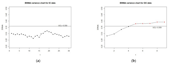
Figure 1. (a) In-control SECOM data; (b) out-of-control SECOM data. The monitoring results of the variance control chart with measurement error for SECOM data.

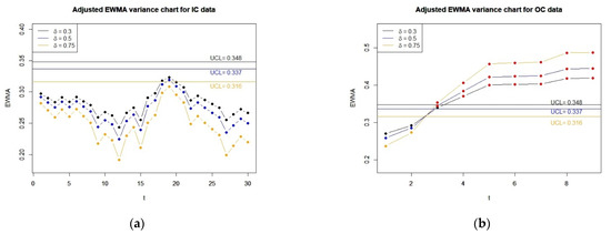
Figure 2. (a) In-control SECOM data; (b) out-of-control SECOM data. The monitoring results of the error-corrected control chart for SECOM data.

5. Conclusions

In this paper, we develop a new variance control chart with the correction of measurement error for a distribution-free continuous observed quality variable. Our idea is to consider the EWMA variance chart for a process with non-normal or unknown distribution and investigates the effects of measurement error on the EWMA variance chart. To correct the effects of measurement error, we propose the error-corrected variance control chart. Numerical results justify the validity of the proposed error-corrected variance control chart. The control limits of the error-corrected EWMA variance chart are more reliable, and the corresponding out-of-control detection ability is very close to the EWMA variance chart without measurement error. On the contrary, without suitable correction of measurement error effects, we find that the control limits and the out-of-control detection ability of the variance control chart with measurement error are extremely unreliable, especially when moderate and large levels of measurement error are involved. As commented by a referee, it is interesting to compare with other existing methods to show the advantages of our proposed method. However, to the best of our knowledge, few methods have been available to correct for measurement error effects when constructing control charts. We will keep exploring alternative approaches and then compare them with our method in the near future.

References

- Shewhart, W.A. Some applications of statistical methods to the analysis of physical and engineering data. Bell Syst. Tech. J. 1924, 3, 43–87. [Google Scholar] [CrossRef]
- Roberts, S.W. Control chart tests based on geometric moving averages. Technometrics 1959, 1, 239–250. [Google Scholar] [CrossRef]
- Amin, R.W.; Reynolds, M.R., Jr.; Saad, B. Nonparametric quality control charts based on the sign statistic. Commun. Stat. Theory Methods 1995, 24, 1597–1623. [Google Scholar] [CrossRef]
- Bakir, S.T. A distribution-free Shewhart quality control chart based on signed-ranks. Qual. Eng. 2004, 16, 613–623. [Google Scholar] [CrossRef]
- Bakir, S.T. Distribution-free quality control charts based on signed-rank-like statistics. Commun. Stat.-Theory Methods 2006, 35, 743–757. [Google Scholar] [CrossRef]
- Yang, S.F.; Lin, J.S.; Cheng, S.W. A new nonparametric EWMA sign control chart. Expert Syst. Appl. 2011, 38, 6239–6243. [Google Scholar] [CrossRef]
- Yang, S.F.; Cheng, T.C.; Hung, Y.C.; Cheng, S.W. A new chart for monitoring service process mean. Qual. Reliab. Eng. Int. 2012, 28, 377–386. [Google Scholar] [CrossRef]
- Chowdhury, S.; Mukherjee, A.; Chakraborti, S. A new distribution-free control chart for joint monitoring of unknown location and scale parameters of continuous distributions. Qual. Reliab. Eng. Int. 2014, 30, 191–204. [Google Scholar] [CrossRef]
- Yang, S.F.; Arnold, B.C. A simple approach for monitoring business service time variation. Sci. World J. 2014, 2014, 238719. [Google Scholar] [CrossRef]
- Yang, S.F.; Arnold, B.C. A new approach for monitoring process variance. J. Stat. Comput. Simul. 2016, 86, 2749–2765. [Google Scholar] [CrossRef]
- Tang, A.; Castagliola, P.; Hu, X.; Sun, J. The adaptive EWMA median chart for known and estimated parameters. J. Stat. Comput. Simul. 2019, 89, 844–863. [Google Scholar] [CrossRef]
- Riaz, M.; Abid, M.; Shabbir, A.; Nazir, H.Z.; Abbas, Z.; Abbasi, S.A. A non-parametric double homogeneously weighted moving average control chart under sign statistic. Qual. Reliab. Eng. Int. 2021, 37, 1544–1560. [Google Scholar] [CrossRef]
- Mittag, H.-J.; Stemann, D. Gauge imprecision effect on the performance of the control chart. J. Appl. Stat. 1998, 25, 307–317. [Google Scholar] [CrossRef]
- Linna, K.W.; Woodall, W.H. Effect of measurement error on Shewhart control charts. J. Qual. Technol. 2001, 33, 213–222. [Google Scholar] [CrossRef]
- Stemann, D.; Weihs, C. The EWMA-XS-control chart and its performance in the case of precise and imprecise data. Stat. Pap. 2001, 42, 207. [Google Scholar] [CrossRef]
- Maravelakis, P.; Panaretos, J.; Psarakis, S. EWMA chart and measurement error. J. Appl. Stat. 2004, 31, 445–455. [Google Scholar] [CrossRef]
- Abbas, N.; Riaz, M.; Does, R.J. An EWMA-type control chart for monitoring the process mean using auxiliary information. Commun. Stat. Theory Methods 2014, 43, 3485–3498. [Google Scholar] [CrossRef]
- Daryabari, S.A.; Hashemian, S.M.; Keyvandarian, A.; Maryam, S.A. The effects of measurement error on the MAX EWMAMS control chart. Commun. Stat. Theory Methods 2017, 46, 5766–5778. [Google Scholar] [CrossRef]
- Noor-ul-Amin, M.; Riaz, A.; Safeer, A. Exponentially weighted moving average control chart using auxiliary variable with measurement error. Commun. Stat. Simul. Comput. 2020, 51, 1002–1014. [Google Scholar] [CrossRef]
- Asif, F.; Khan, S.; Noor-ul-Amin, M. Hybrid exponentially weighted moving average control chart with measurement error. Iran. J. Sci. Technol. Trans. A Sci. 2020, 44, 801–811. [Google Scholar] [CrossRef]
- Huwang, L.; Hung, Y. Effect of measurement error on monitoring multivariate process variability. Stat. Sin. 2007, 17, 749–760. [Google Scholar]
- Nojavan, M.; Alishahi, M.; Rezaee, M.; Rahaee, M.A. The effect of measurement error on the performance of Mann-Whitney and Signed-Rank nonparametric control charts. Qual. Reliab. Eng. Int. 2021, 37, 2365–2383. [Google Scholar] [CrossRef]
- Case, K.E.J. The control chart under inspection error. J. Qual. Technol. 1980, 12, 1–9. [Google Scholar] [CrossRef]
- Lu, X.S.; Xie, M.; Goh, T.N. An investigation of the effects of inspection errors on the run-length control charts. Commun. Stat. Simul. Comput. 2000, 29, 315–335. [Google Scholar] [CrossRef]
- Shu, M.-H.; Wu, H.C. Monitoring imprecise fraction of conforming items using p control charts. J. Appl. Stat. 2010, 37, 1283–1297. [Google Scholar] [CrossRef]
- Daryabari, S.A.; Malmir, B.; Amiri, A. Monitoring Bernoulli processes considering measurement errors and learning effect. Qual. Reliab. Eng. Int. 2019, 35, 1129–1143. [Google Scholar] [CrossRef]
- Chen, L.-P.; Yang, S.-F. A new p-control chart with measurement error correction. Qual. Reliab. Eng. Int. 2023, 23, 81–98. [Google Scholar] [CrossRef]
- McCann, M.; Johnston, A. UCI Machine Learning Repository. Available online: https://archive.ics.uci.edu/ml/datasets/SECOM (accessed on 1 December 2021).
Disclaimer/Publisher’s Note: The statements, opinions and data contained in all publications are solely those of the individual author(s) and contributor(s) and not of MDPI and/or the editor(s). MDPI and/or the editor(s) disclaim responsibility for any injury to people or property resulting from any ideas, methods, instructions or products referred to in the content. |
© 2023 by the authors. Licensee MDPI, Basel, Switzerland. This article is an open access article distributed under the terms and conditions of the Creative Commons Attribution (CC BY) license (https://creativecommons.org/licenses/by/4.0/).