Article

A Study on the Methodology for Estimating Floating Population in Microscopic Spatial Units

1
Department of Urban and Regional Development, Mokpo National University, Muan-gun 58554, Jeollanam-do, Republic of Korea
2
Centre for Small Business Insights, Seoul Credit Guarantee Foundation, Mapo-gu, Seoul 04130, Republic of Korea
*
Author to whom correspondence should be addressed.
Sustainability 2023, 15(5), 4407; https://doi.org/10.3390/su15054407
Submission received: 17 January 2023 / Revised: 17 February 2023 / Accepted: 22 February 2023 / Published: 1 March 2023

Abstract

:
Estimating pedestrian volume has become an important topic in urban planning and transportation-planning research. However, current models find it difficult to predict long-term changes in pedestrians due to changes in land use and transport infrastructure. In this study, a methodology was devised to estimate the mesoscale pedestrian volume according to the results of a long-term-forecasting model integrating land use and transportation. The methodology was validated using pedestrian volume data collected from Gangnam, Seoul. The main contributions of this study are that the proposed methodology enables the long-term prediction of mesoscale pedestrian volume, which has previously been difficult to analyze, and that it considers not only pedestrians who are walking but also public transportation users moving between public transport nodes and buildings. Thus, it can accommodate long-term changes in not only land use but also in transportation infrastructure.

1. Introduction

Walking is the most fundamental means of transportation for human beings and is an essential act for using city facilities, including various activities [1]. Even though motor vehicles are the main means of transportation today, walking is still the basic and universal means of transportation for individuals [2,3,4]. Walking is performed at the beginning and end of a trip; thus, it is an indispensable means for humans to move for any purpose [5,6]. People walk to move in urban spaces and make a living. Pedestrians represent the liveliness of an urban area [7,8]. Although walking is the most basic and important means of transportation, it has been neglected because cities are planned to increase the mobility of automobiles. In particular, changes in a transportation system centered on road infrastructure facilities affect the mode choices of passengers, resulting in a decrease in pedestrian traffic [9,10]. There have been studies that criticize car-oriented urban planning as not sustainable [11,12]. Compact cities and transit-oriented development (TOD) have recently attracted attention as an important paradigm of urban development. Walking has been evaluated as an index for measuring the sustainability of a city beyond merely a means of traffic [13,14,15,16,17]. Therefore, estimating pedestrian volume has become an important topic for urban planning and transportation-planning research [14,18,19,20].
There are two approaches to research pedestrian volume modeling [21,22]. The route choice model follows the conventional four-step travel model that is widely used in transportation planning: trip generation, trip distribution, modal split, and traffic assignment. The four-step model has long been commonly used for estimating motorized vehicles [22]. Conventionally, four-step travel models have been modified to include pedestrian mode choices [23,24]. Some studies have emphasized that several other steps should be considered to estimate non-motorized transportation modes [21,25]. However, these models are typically applied to traffic analysis zones; this is a geographic scale that is too large to capture fine-grained differences in pedestrian activity at individual intersections [21]. Clifton et al. [26] overcame this limitation by estimating pedestrian trip generation, trip distribution, and route assignment between block-sized pedestrian analysis zones in central Baltimore. However, their model did not include pedestrians moving to use public transportation, and they make up a large proportion of pedestrians.
The second approach is to construct models within the conceptual and methodological framework of space syntax. These models are based on the following contention, as has been demonstrated in many studies: the configuration of a street network determines to a large extent the distribution of movement within it. This theoretical framework is based on a topological visual analysis of a street network called an axial map; this is defined as the smallest set of straight axial lines covering an urban street network. The integration (i.e., accessibility) level of each axial line within a network is then computed by space syntax centrality measures that apply a graph analysis to the axial map in order to represent the movement potential in the street network. Such an analysis allows the built environment to be modeled in a way that reflects how it is perceived by people on the ground [27]. Many studies have used this methodology to analyze pedestrians in urban areas in, for example, Atlanta [28]; Oakland, CA [29]; Istanbul [30]; Seoul [31]; Santa Maria, Brazil [32]; Tel Aviv and Bat Yam, Israel [33]; and Fukuoka, Japan [34]. However, these models find it difficult to predict long-term changes in pedestrians owing to changes in land use and transport infrastructure.
Walking volume is difficult to predict for long-term periods because it is influenced not only by the land use and network structure in an urban space but also by the socioeconomic factors of activities. In particular, existing research methods are limited in predicting long-term changes in activities at meso- or microscale levels, such as walking. These limitations have also been observed in various research areas targeting meso- or microscale spaces, in addition to pedestrian volume modeling. A methodology to overcome these limitations is needed. Consequently, analytical methodologies have been developed for predicting meso- or microscopic spatial areas by simulating long-term changes in macroscale units, such as the PROPOLIS [35] and ILUMASS [36] projects. These approaches have been used to estimate various results at the mesoscale level [37,38,39]. However, research on estimating the pedestrian volume of a network in relation to the liveliness and sustainability of an urban area is still insufficient because of the absence of suitable data and analysis methodology.
In this study, the four-step model is partially amended to devise a pedestrian volume estimation method based on the analysis results of a macroscale model. This methodology is verified using pedestrian volume data collected from 10,000 sites in 2009 by the Seoul Metropolitan Government. The proposed model can be used for predicting long-term pedestrian volume at the mesoscale level.

2. Analytical Framework

2.1. Selection of Case Studies

This study focused on Gangnam-gu and Seocho-gu (hereafter, Gangnam area) in Seoul for analysis. As shown in Figure 1, the Gangnam area is located in the southeast of Seoul and has undergone rapid urbanization since the late 1960s through government-led development [40,41]. The Gangnam area is representative of Korea’s compact urbanization and has the most concentrated, largest floating population in Korea. The Gangnam area consists of 2 gu and 40 dong districts (gu and dong are administrative space division units defined in Korea; Seoul consists of 25 gu and 424 dong) and includes 36 subway stations and 885 bus stops. As of 2010, the Gangnam area had approximately 910,000 residents, 75,000 buildings, and 1 million jobs.
The analysis was based on 2010 because this was the most recent year of household travel survey data that was disclosed by the Korea Transport DB Center. In addition, the analysis time interval was limited to the morning peak hours, which is when most essential trips occur.

2.2. Methods

A methodology was devised and verified for estimating the pedestrian volume in a mesoscale region. Traffic and land-use indicators derived from a macroscale land use and transport model were used for each zone. The methodology of analyzing meso- or microscale sites based on the results of a macroscale model not only uses the results of the macroscale model more efficiently but also allows long-term changes in the meso- and microscale regions to be predicted [37,38,39].
The four-step model is used to estimate the pedestrian volume at the mesoscale. This has been the dominant approach for demand modeling of people traveling. The initial development of models for trip generation, distribution, and diversion in the early 1950s led to the first comprehensive application of the four-step model to transportation in the Chicago area [42]. The pedestrian volume calculation algorithm in this study was designed by adjusting the four-step model for trip generation, mode choice, trip distribution, and trip assignment.
In the trip generation step, a multinomial regression analysis is performed to calculate the trip generation unit for each purpose. The dependent variables of the analysis are based on the produced and attracted traffic volumes for each zone, which can be calculated with the macroscale model. The independent variables are based on the land use areas and socioeconomic indicators for each zone, which can be calculated with the macroscale model. The number of produced and attracted trips for each building are derived based on the calculated basic units. The land area of each building can be calculated according to long-term changes in microspatial units based on the results of the macroscale model and are utilized to calculate the traffic volume for each building.
In the mode choice step, the traffic volume by mode of each building is analyzed using the mode-sharing ratio of each zone, which can be calculated with the macroscale model. This methodology makes it possible to apply the characteristics of each region in the macroscale model to the mesoscale model.
The destination selection step defines the origin and destination points of pedestrians for each building. Pedestrian volume is defined as traffic from public transport and people walking by each building. The destinations of public transportation users and destination radii of walkers were defined through a literature review.
In the trip assignment step, the traffic between each building and the traffic origin or destination are calculated and allocated to the network. Similar to the destination choice step, traffic is classified into two types: public transportation and walking. The traffic volume is assigned according to the gravity model and characteristics of each trip purpose. In particular, public transportation users are assigned by utilizing the number of people entering and exiting at each bus stop (subway station), which can be calculated from the land use and transport model.
The pedestrian volume of each network was calculated with the above four-step analysis, and the validation was performed with actual pedestrian volume data. The results were used to demonstrate the explanatory power and limitations of the methodology.

3. Analysis

3.1. Trip Generation

The trip generation step consisted of two phases: calculating the basic units of the produced and attracted trips for each land use and calculating the produced and attracted traffic for each building. In order to calculate the basic unit of trip generation for each land use, a multinomial regression analysis was carried out. The produced and attracted trips of 424 zones were used as dependent variables, and land use area of each type and the socioeconomic index were used as independent variables. Trips were classified into four purposes: home-based work (HBW), home-based school (HBS), home-based other (HBO), and non-home-based (NHB). Each trip purpose was divided into two types: production (P) and attraction (A).
For the home-based trip production model, the land use area was determined using the type of housing, population ratio, and land price of each zone as independent variables. For the home-based trip attraction model and non-home-based trip model, the land-use area was selected using the nonresidential use of each zone as an independent variable. The ratios of jobs by type of industry and students by type of school were selected as independent variables for trip purpose. This was formulated as follows:
T V i T P   P A = α T P   P A + L U β L U T P   P A · L U i + S E β S E T P   P A · S E i
where T V i T P   P A is the traffic volume by trip purpose (TP) and trip type (PA) in area i; L U i is the total area by land use type (LU) in area i; S E i is the factor of the socioeconomic type (SE) in area i; α T P   P A is the constant by trip purpose (TP) and trip type (PA); β L U T P   P A is the land use parameter (LU) by traffic purpose (TP) and traffic type (PA); and β S E T P   P A is the socioeconomic parameter (SE) by traffic purpose (TP) and traffic type (PA). TP is the trip purpose (HBW, HBS, HBO, or NHB); PA is the trip type (P or A); LU is the total floor area by land use type The total floor area could be classified as residential nonresidential use. Residential land use was divided into detached houses, multihouses, official residences, apartments, row houses, multiplex houses, and dormitories. Nonresidential land use was divided into type-1 neighborhood living facilities, type-2 neighborhood living facilities, cultural assembly facilities, religious facilities, sales facilities, transportation facilities, medical facilities, education and research facilities, elderly or children facilities, training facilities, sports facilities, office facilities, accommodations, recreational facilities, factories, storage facilities, hazardous material storage facilities, automobile-related facilities, animal- or plant-related facilities, excrement disposal facilities, correctional or military facilities, communication facilities, power facilities, cemetery facilities, tourism and leisure facilities, temporary buildings, funeral halls, neighborhood living facilities, sales and business facilities, education and research or welfare facilities, and public facilities. SE represents the socioeconomic factors (population ratios by age group, land price, percentage of jobholders by eighteen, industry type, and numbers of students accepted by four school types). Population age groups were classified as 10–19 years old, 20–34 years old, 35–49 years old, 50–64 years old, and 65 years or over. The industry types used to estimate the numbers of jobs were agriculture, forestry, fishery, mining, manufacturing, electricity, gas, steam, water supply, wastewater treatment, raw material recovery, environmental restoration, construction, wholesale, retail, transportation, accommodation or restaurant, publishing or video and broadcasting communication and information service, finance and insurance, brokerage and leasing of real estate, science and technology service, public and social security administration or defense, education service, health and social welfare services, arts, sports and leisure services, associations and organizations, and repair or other personal services. School types were divided into elementary, middle, high, and university or higher (see Figure 2).
The multinomial regression analysis only yielded significant independent variables through backward deletion. Table 1 presents the results of the home-based trip production model, and Table 2 presents the results of the home-based trip attraction and non-home-based trip models.
The parameters calculated from the multiple regression analysis, land use area, and socioeconomic index for each building were used to calculate the produced and attracted traffic volumes for each building:
T V k T P   P A = L U β L U T P   P A · L U k + α T P   P A + S E β S E T P   P A · S E k K T P   P A
where T V k T P P A is the traffic volume by trip purpose (TP) and trip type (PA) for building k; β L U T P   P A is the land use parameter (LU) by traffic purpose (TP) and traffic type (PA); β S E T P   P A is the socioeconomic parameter (SE) by traffic purpose (TP) and traffic type (PA); L U k is the total area by land use (LU) of building k; S E k is the socioeconomic (SE) factor of building k; and K T P   P A is the total number of buildings producing or attracting trips according to the traffic purpose (TP) and traffic type (PA) in the zone where building k is located. TP is the trip purpose (HBW, HBS, HBO, or NHB); PA is the trip type (P or A); and LU is the total floor area by land use type. Figure 3 shows the calculated traffic volumes produced and attracted by each building.

3.2. Mode Choice

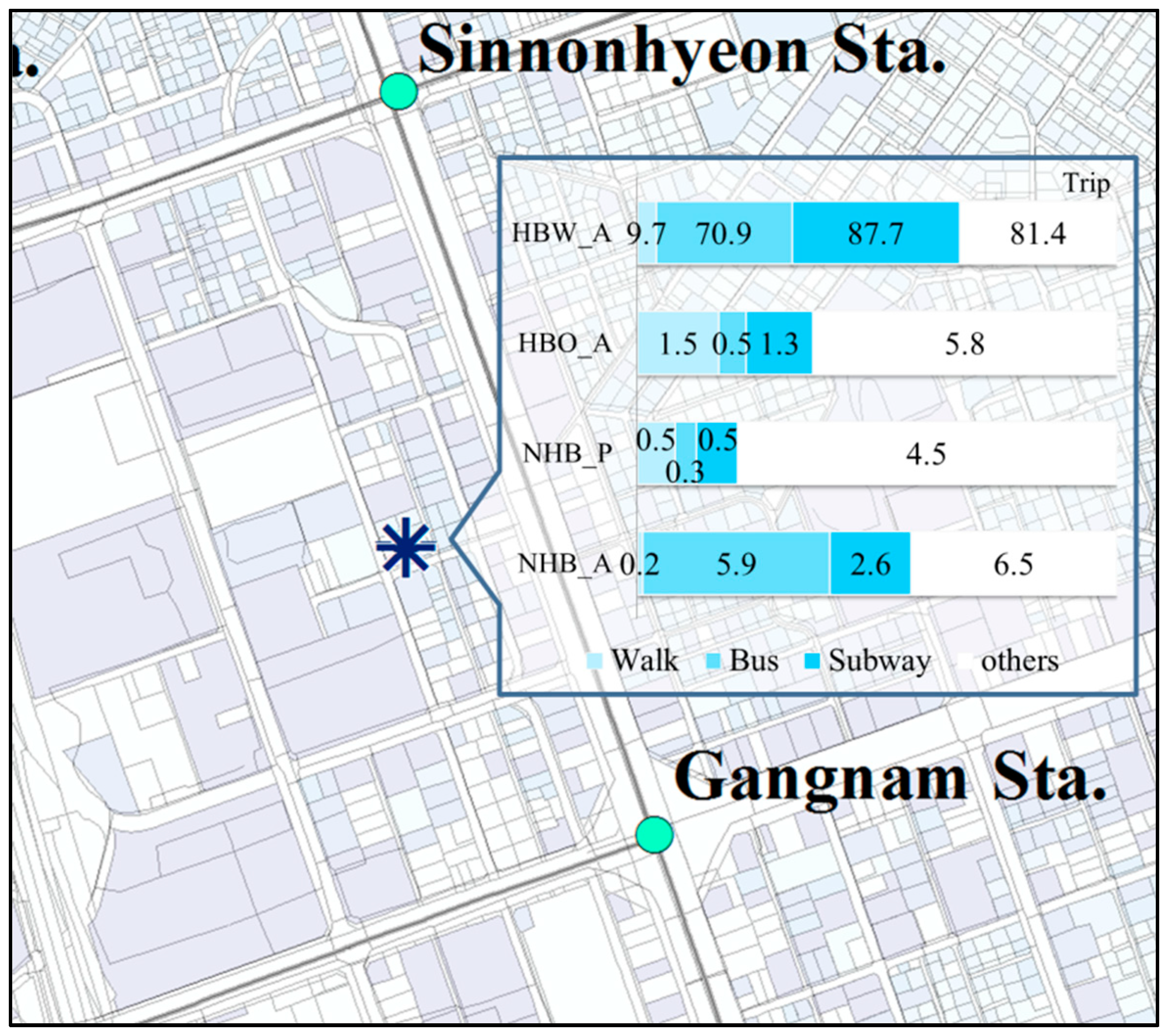
The mode choice model used the mode share results for each zone calculated from the macroscale model. The mode share data were divided according to trip purpose and trip type. Through this methodology, the mode share characteristics for each zone derived from the macroscale model were applied to the mesoscale area analysis model. The purpose of this study was to estimate the distribution and density of the floating population in the mesoscale area. Therefore, only walking and public transportation trips related to pedestrians were defined as the analytical target, and the traffic volumes were extracted. The average mode share rates of 40 zones in the Gangnam area are shown in Figure 4. The walking and public transport traffic volumes for each building were calculated as shown in Figure 5 based on the mode-sharing ratio of the zone to which each building belonged.

3.3. Destination Choice

The destination choice step consisted of defining the destination point of the produced traffic in each building and the origin point of the attracted traffic from each building. The destination and origin points of pedestrians who used public transport in each building were the bus stop or subway station (i.e., public transportation nodes). In addition, the destination and origin points of people walking in each building were buildings.
The distance criterion for moving between buildings or between buildings and public transportation nodes was based on indicators presented in the report by the Korea Transport Institute (KOTI). The walking distance between a building and public transportation node was set to 1 km in reference to the public transportation access and egress distance criteria for constructing the traffic demand estimation model of the KOTI. The walking distance between buildings was set to 2 km in reference to the walking area criteria for constructing the traffic demand estimation model of the KOTI [43]. Figure 6 shows the destination of each building selected during the destination choice step.

3.4. Trip Assignment

In the trip assignment step, trips were divided into two types: public transportation and walking. Public transport trips were divided into buses and subways and were performed by passengers traveling between public transportation nodes and buildings. Walking traffic referred to pedestrians traveling between buildings on foot.

3.4.1. Trip Assignment Model for Public Transport

Based on the criteria set in the destination choice step, public transportation nodes located within 1 km of the network distance of each building were defined as the origin and destination points of traffic. The shortest route was derived through a network analysis of the arc map and defined as the route between each building and the public transportation node. In the case of vehicle trips, the route was defined while considering delays and charges. However, delays and charges were not considerations for walking. In addition, the Gangnam area was connected to the outside area and could be freely entered and exited through walking. Therefore, the trip assignment analysis included buildings and public transportation nodes within 1 km outside the analysis area.
The amount of traffic between a building and public transportation node was calculated with a gravity model based on the distance between the two points and the number of people entering and exiting at each public transportation node; this was calculated with the land use and transport model. Equations (3) and (4) show the calculation for the traffic between buildings and bus stops:
B k s P = B k P · G N s / D I k s 2 n G N n / D I k n 2
B k s A = B k A · G F s D I k s 2 n G F n D I k n 2
where B k s P and B k s A is the bus traffic between bus stop s and building k that is produced (P) or attracted (A) by building k, respectively; B k P and B k A is the bus traffic produced (P) or attracted (A) by building k, respectively; G N s and G F s are the numbers of people entering (GN) or exiting (GF) bus stop s; respectively D I k s is the distance between building k and bus stop s; and n is all the alternate bus stops for building k (within a network distance of 1 km).
The traffic between buildings and subway stations was calculated in the same manner as the bus traffic. The calculated traffic volume between buildings and public transportation nodes was input to the walking route connecting the two points.
Figure 7 shows the number of passengers using public transportation nodes. Figure 8 and Figure 9 show the number of public transportation users who were allocated by the gravity model based on the distance between two points and the number of people entering and exiting at each public transportation node, respectively.

3.4.2. Trip Assignment Model for Walking Trips

Based on the criteria set in the destination choice step, buildings located within a network distance of 2 km were defined as the origin and destination points of walking traffic. In addition, the Gangnam area was connected to the outside area and could be freely entered and exited by walking. Therefore, the trip assignment analysis included buildings within 2 km outside the analysis area.
The walking traffic produced and attracted by each building was divided according to the trip purpose. The trip assignment model assigned walking trips based on the distribution characteristics of each trip purpose. The walk distribution characteristics were analyzed based on traffic volume according to the distance between the origin and destination points. The characteristics for each purpose were calculated as an exponential function, as shown in Figure 10. The analysis of the walking characteristics for each trip purpose showed that HBS traffic (approximately 53%) was more frequent than other purposes for short distances (0–500 m). On the other hand, NHB traffic (approximately 9%) had the most people traveling long distances (1500–2000 m) compared to the other purposes.
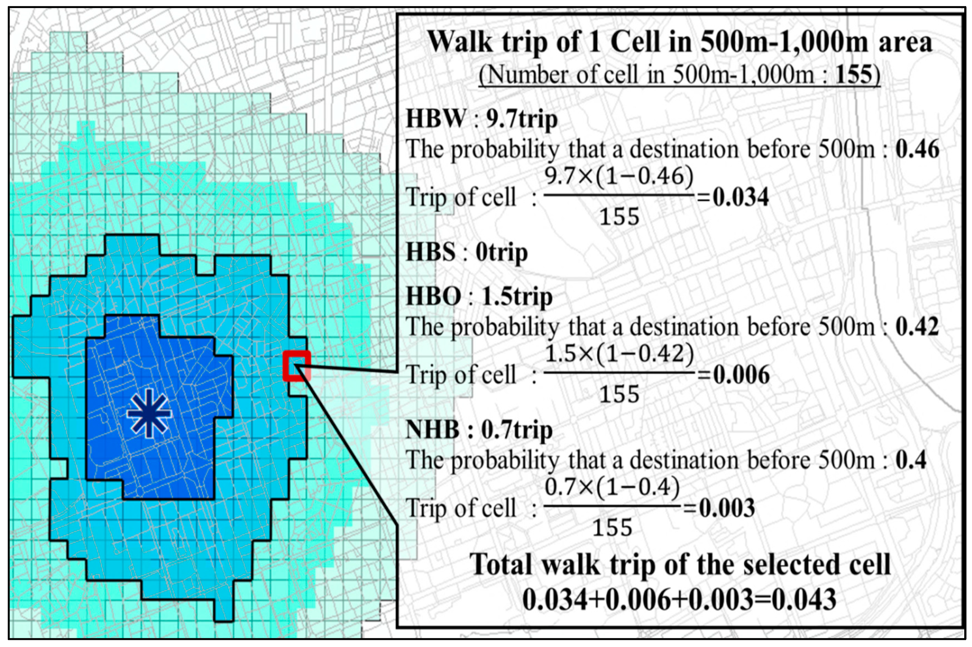
In order to assign walking traffic, a service area analysis of the arc map was used to divide the surrounding area of each building into equidistant areas. As shown in Figure 11, the network area was divided into distance increments of 500 m in four areas: 500, 1000, 1500, and 2000 m. The walking traffic was input in each network area by considering the walking distribution characteristics of each trip purpose. Each network area was divided into 100 m × 100 m cells, and traffic input into the network area was allocated equally to each cell. The walking traffic of each cell was calculated as follows:
W k c = T P W V k T P · ( 1 - W C c T P ) N C c
where W k c is the number of walking trips of building k allocated to the cell belonging to the network area class (c); W V k T P is the volume of walking trips of building k for each trip purpose (TP); TP is the trip purpose (HBW, HBS, HBO, or NHB); c is the network area class (0–500, 500–1000, 1000–1500, or 1500–2000 m); W C c T P is the ratio of walking traffic distributed to each network area class (c) by each trip purpose (TP) ( W C 0 - 500 m H B W : 0; W C 500 - 1000 m H B W : 0.46; W C 1000 - 1500 m H B W : 0.71; W C 1500 - 2000 m H B W : 0.85; W C 0 - 500 m H B S : 0; W C 500 - 1000 m H B S : 0.53; W C 1000 - 1500 m H B S : 0.78; W C 1500 - 2000 m H B S : 0.90; W C 0 - 500 m H B O : 0; W C 500 - 1000 m H B O : 0.42; W C 1000 - 1500 m H B O : 0.66; W C 1500 - 2000 m H B O : 0.80; W C 0 - 500 m N H B : 0; W C 500 - 1000 m N H B : 0.40; W C 1000 - 1500 m N H B : 0.64; and W C 1500 - 2000 m N H B : 0.79); and N C c is the number of cells in the network area class (c). Figure 12 shows the calculated results of the walking traffic for each cell.

4. Validation

This study was validated using survey data of pedestrians at 10,000 points from 2009 gathered by the Seoul Metropolitan Government. The Gangnam area, which was the scope of this study, included 1284 survey points. The survey was conducted on Tuesday, Friday, and Saturday from 7 am to 21 pm. This study utilized data collected from 7 am to 10 am on Tuesday. The average pedestrian volume was 605, with a maximum of 6615 and a minimum of 0 (one spot).
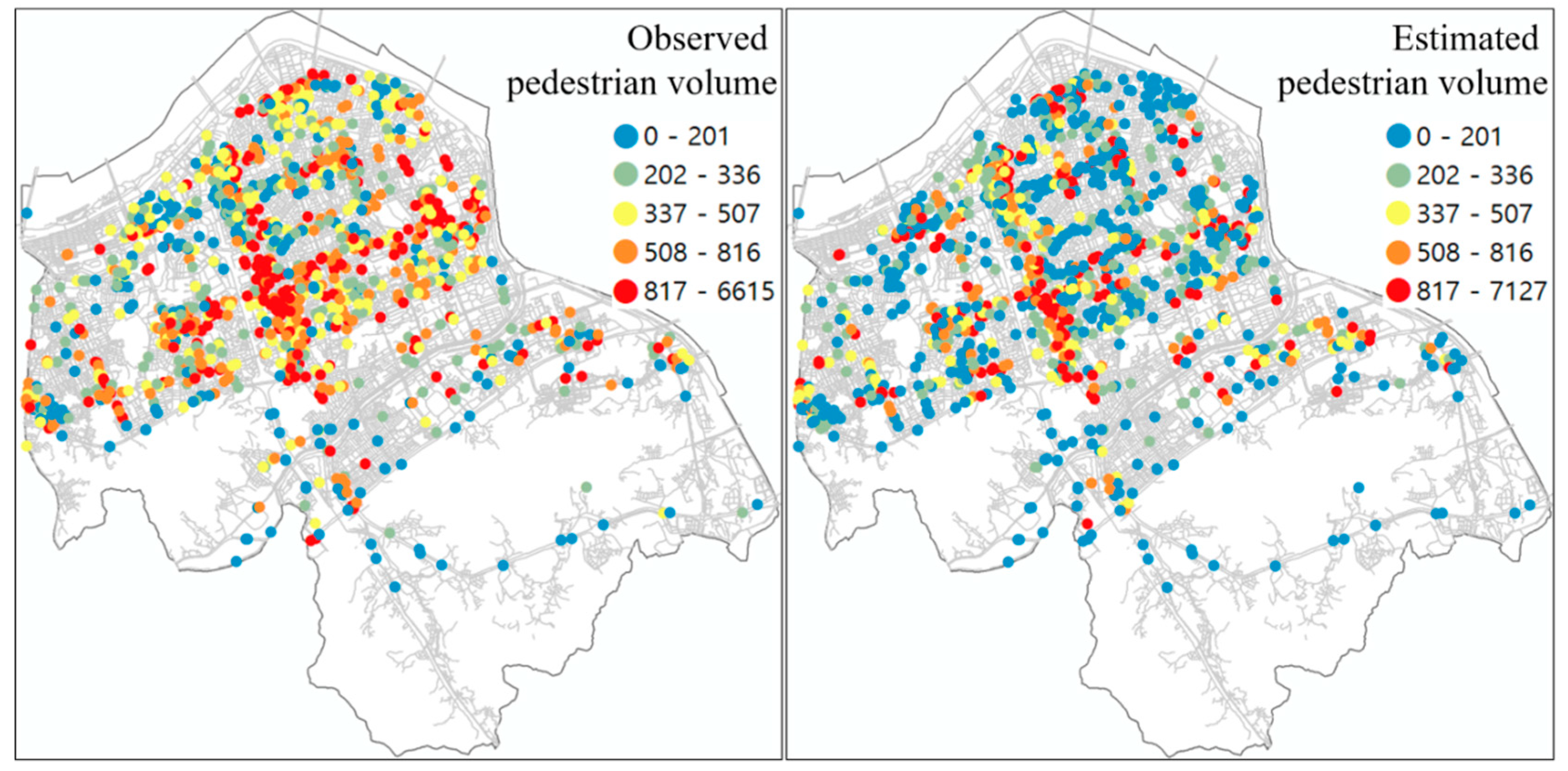
Pedestrian volume was estimated at the same points as the survey points. The pedestrian volume of each point was estimated by summing the allocated public transport and walking traffic in the network. Figure 13 shows a simple conceptual diagram of the calculation method for each point’s pedestrian volume. The estimated pedestrian volume of each point was 20.23% more than the observed data. The average estimated pedestrian volume and observed data were matched through the validation process to adjust the estimated pedestrian volume. Figure 14 shows the observed and estimated pedestrian volumes at each survey point.
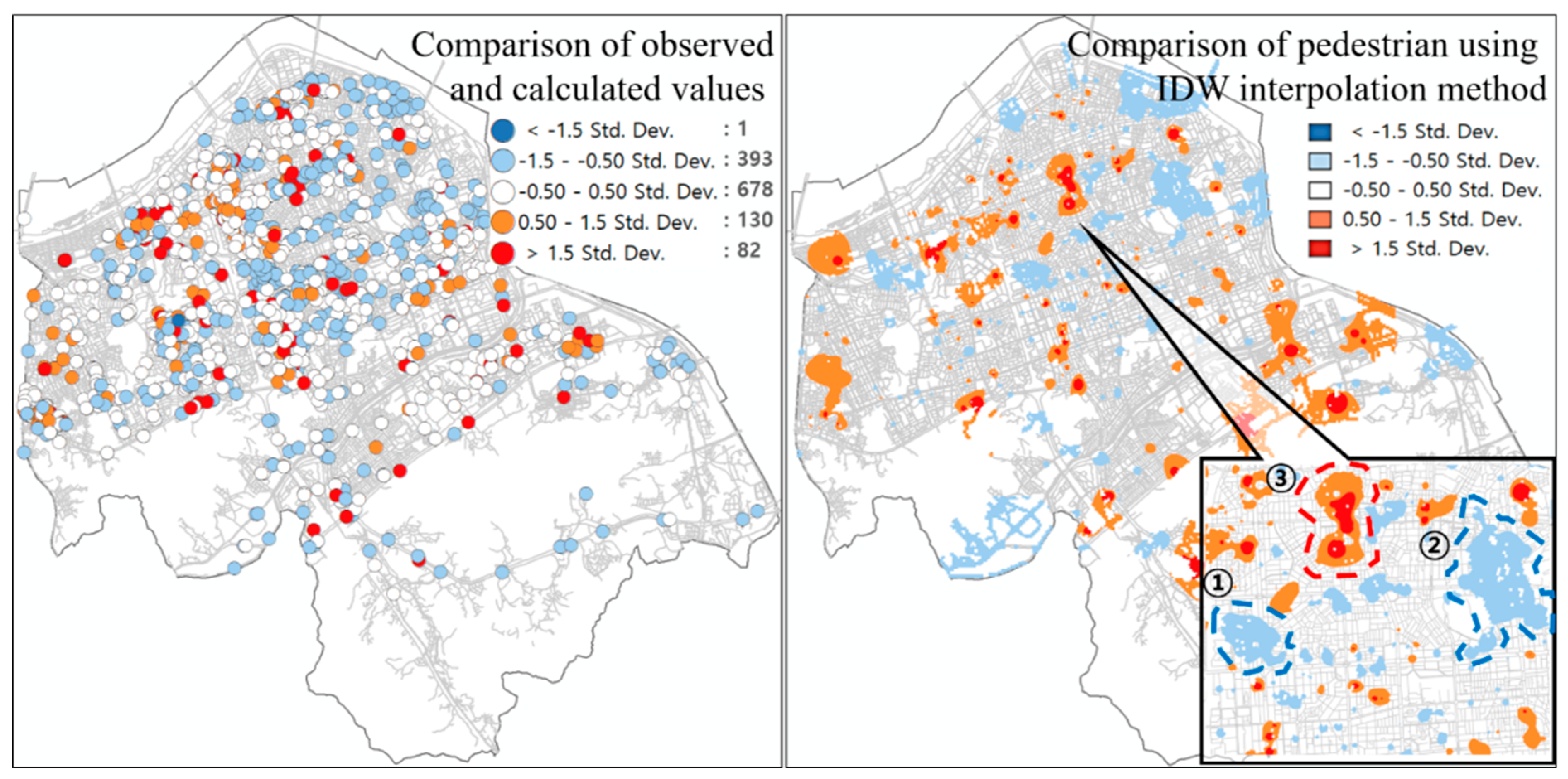
Figure 15 compares the observed pedestrian volume and estimated data for each observation point. Out of 1284 observations, 678 estimates (52.8%) were within ±0.5 of the standard deviation (±58.80%) of the observed data. This result indicates that the methodology of this study estimated the pedestrian volume within approximately ±60% of the observed data at half of the analysis sites. In addition, the estimated pedestrian volume was within ±1.5 times the standard deviation (±176.41%) of the observed pedestrian volume at 1201 of 1284 observation points (93.5%). This means that the methodology estimated the pedestrian volume within approximately ±180% of the observed data for most of the analyzed area.
Figure 16 compares the observed and estimated pedestrian volumes for each observation point in the Gangnam area. The analysis area was interpolated through the inverse distance-weighted (IDW) analysis provided by the arc map to select areas where pedestrian volume was excessive or underestimated.
The suburbs of the Gangnam area had few pedestrian survey points, which greatly affected the analysis results. Therefore, only the center of the Gangnam area was considered for reliable interpolation results because of the many pedestrian survey points.
When the IDW analysis was used to interpolate the estimated pedestrian volume, most of the Gangnam central area was within ±0.5 of the standard deviation (±58.80%) for the observed pedestrian volume. This means that the analytical methodology was quite reliable at estimating the pedestrian volume. However, pedestrians were overestimated or underestimated at three places. The reasons are given below.
Area ① was the section between the interstate bus (a bus that runs through more than two cities and connects the surrounding city with the city center of the big city) stop and Gangnam station, and the pedestrian volume was underestimated compared with the observed data. Approximately 240 interstate bus lines connecting Seoul and Gyeonggi-do (Gyeonggi-do surrounds Seoul and is the most populous area (about 11.8 million) in Korea (as of 2010)) or Incheon metropolitan city (Incheon metropolitan city is located west of Gyeonggi-do and is connected to Seoul to the east; Incheon metropolitan city has a population of about 2.8 million and is the third-most populous city in Korea (as of 2010)) pass through the Gangnam area. Many passengers enter or exit at the interstate bus stop in area ①. Some users of the interstate buses are traveling to the Gangnam area, but most are transferring through the area to travel to other parts of Seoul. Thus, many pedestrians walk between the bus stop and the subway station. However, the methodology had limitations when estimating transferring pedestrians because the pedestrian volume was calculated based on the land use of the analysis area. This is why the pedestrian volume in area ① was underestimated.
Area ② contained the Korea General Trade Center, which holds various domestic and international exhibitions and conferences. The pedestrian volume in the area was underestimated relative to the observed data. This is because the analytical methodology did not adequately estimate pedestrians attracted by the Korea General Trade Center. This study used the traffic volumes and land use areas of 424 zones in Seoul to calculate the traffic volumes produced and attracted by each building. However, it was very difficult to estimate the traffic volume attracted by the Korea General Trade Center with this methodology because of its uniqueness. This is why the pedestrian volume in area ② was underestimated.
The pedestrian volume of area ③, which was the side streets of Hak-dong station, was overestimated in comparison with the observed data. This was because of the physical characteristics of the buildings in this area. Unlike the Gangnam area, where large buildings are concentrated, the side streets of Hak-dong station have small-sized buildings. In 2010, which was the timeframe of the analysis, the vacancy of small- and medium-sized buildings in the Gangnam area was a big problem. In the fourth quarter of 2010, the vacancy rate of premium-grade buildings (floor area of 66,000 m2 or more) was 1.8%, while that of class-C buildings (less than 16,500 m2) was 7.86%. The average office vacancy rate in the Gangnam area was 6.27%. The methodology had limitations in analyzing the decrease in pedestrian volume due to vacancy because it calculated the traffic volume based on the land-use area. This is why the pedestrian volume in area ③ was overestimated.

5. Concluding Remarks

5.1. Discussion

As a result of reviewing previous studies, there are two main ways to estimate the floating population. The method using the traditional transport model has limitations in estimating the floating population on a walking path because it takes the macroscopic space as the unit of analysis, whereas the methodology for estimating floating population using space syntax has limitations in estimating long-term changes in traffic. This study proposed a methodology for estimating pedestrian volume based on the analysis results of a macroscale model. The methodology partially amended the four-step model for estimating pedestrian volume. The traffic produced and attracted by each building was calculated in the trip generation step and divided by each mode. The trip destinations were defined based on the user characteristics of each mode and were used to assign the pedestrian volume to the walking network. In this study, only traffic for public transportation and walking between buildings were assumed to make up the pedestrian volume in the network.
The analysis methodology of this study estimated long-term changes in traffic by utilizing the output of a traffic model. The floating population was calculated considering the environment of the microscopic space unit. As a result, it overcame the limitations of existing research. Therefore, this research model presented the floating population in a microscopic spatial area, which is difficult to present in a study that estimates long-term traffic changes based on a transport model [21,26]. In addition, since this research model was based on the results of a macroscale model, it was possible to present a future floating population that cannot be estimated in studies using space syntax [28,29,30,31,32,33,34].
The methodology was verified using pedestrian volume data collected from the Gangnam area in Seoul. The validation results showed that the methodology estimated the pedestrian volume within approximately ±60% (i.e., half the standard deviation) of the observed data at half of the analysis sites. Furthermore, the pedestrian volume was estimated within approximately ±180% of the observed data (i.e., 1.5 times the standard deviation) in most of the analyzed areas. This means that the analytical methodology was quite reliable at estimating pedestrian volume. However, pedestrian volume was overestimated or underestimated in some places.

5.2. Limitations and Significance of the Study

The limitations of this research methodology were confirmed by examining the characteristics of the overestimated and underestimated regions. First, this research methodology underestimated pedestrian volume due to transfer. Second, it could not estimate the pedestrian volume produced or attracted by a unique building in the analysis area. Finally, the decrease in pedestrian volume due to building vacancy could not be reflected in the analysis.
In addition, this research methodology had limitations caused by using the results of the macroscale model. The macroscale model predicted future traffic volume based on current traffic characteristics. That is, if the future traffic characteristics had a large difference from the present, the error of the predicted traffic volume increased. For example, personal mobility is a travel mode that did not exist in the past. Currently, personal mobility is a new means that has great influence on the mode choice of travelers [44,45]. Therefore, if the current traffic volume was estimated based on the traffic characteristics before personal mobility existed, there would be a big difference from the actual traffic volume.
Nevertheless, this study contributed to pedestrian volume modeling by overcoming the limitations of two existing aspects. First, a methodology was devised for estimating pedestrian volume at the mesoscale level using the results of a long-term-forecasting model integrating land use and transportation. This analytical methodology enabled the long-term prediction of pedestrian volume at the mesoscale level, which has been difficult to analyze before. This methodology may be used not only for pedestrian accidents directly related to pedestrian volume but also for analyzing trade areas, where long-term prediction is considered important. Second, this research methodology included not only people who were only walking but also public transportation users moving between public transport nodes and buildings to estimate the pedestrian volume in the network. Expanding the analysis target pushed the estimation results closer to reality. These advantages allowed the pedestrian volume model to cope with long-term changes in not only land use but also transportation infrastructure.
This study estimated the number of passengers per building through a logical process. Then, using the number of passengers, the floating population on a walking path was calculated. The results calculated through this methodology can be said to be the potential floating population on a walking path. However, there were areas where there was a large gap between the actual and potential floating populations. The reason is that the floating population calculation model presented in this study considered only physical factors. In other words, the model presented in this study did not consider nonphysical factors, such as the culture or stench of a walking path. In addition, it could not predict the volume of a floating population that changed due to nonphysical factors. In the future, we plan to conduct research to identify the specificity of regions where there are large differences between the actual and potential floating populations. In addition to this study, the results of future studies can be used in areas such as the prediction of pedestrian movement and the development of commercial districts in microscopic units.

Author Contributions

Conceptualization, S.J. and Y.A.; methodology, S.J. and Y.A.; software, S.J.; validation, S.J. and Y.A.; formal analysis, S.J.; investigation, S.J. and Y.A.; resources, S.J.; data curation, S.J.; writing—original draft, S.J.; writing—review and editing, Y.A.; visualization, S.J.; supervision, Y.A.; project administration, Y.A.; funding acquisition, S.J. All authors have read and agreed to the published version of the manuscript.

Funding

This work was supported by the Ministry of Education of the Republic of Korea and the National Research Foundation of Korea (NRF-2020R1I1A1A01067265).

Institutional Review Board Statement

Ethical review and approval were waived for this study, as no interventions were included in the data collection about humans.

Informed Consent Statement

Not applicable.

Data Availability Statement

Not applicable.

Conflicts of Interest

The authors declare no conflict of interest.

References

  1. Kim, E.; Choi, E.J.; Yang, J.Y. A study on enhancement methods of level of service analysis for pedestrian sidewalks. J. Korean Soc. Transp. 2015, 33, 29–39. [Google Scholar] [CrossRef] [Green Version]
  2. Lerman, Y.; Rofè, Y.; Omer, I. Using space syntax to model pedestrian movement in urban transportation planning. Geogr. Anal. 2014, 46, 392–410. [Google Scholar] [CrossRef]
  3. Saelens, B.E.; Handy, S.L. Built environment correlates of walking: A review. Med. Sci. Sports Exerc. 2008, 40, S550–S566. [Google Scholar] [CrossRef] [PubMed] [Green Version]
  4. Ferrer, S.; Ruiz, T. Comparison on travel scheduling between driving and walking trips by habitual car users. Transportation 2017, 44, 27–48. [Google Scholar] [CrossRef] [Green Version]
  5. Chung, C.S. A study on the sidewalk space according to the land use: In the zone around main street of Busan Seoul C. B. D. J. Korea Plan. Assoc. 1985, 20, 121–141. [Google Scholar]
  6. Lee, Y.S.; Kang, J.M. A study on urban spatial structure characteristics to influencing factors for revitalization of non-motorized transportation by analyzing—A case of Seoul, Korea. J. Urban Des. Inst. Korea 2013, 14, 5–18. [Google Scholar]
  7. Zook, J.B.; Lu, Y.; Glanz, K.; Zimring, C. Design and pedestrianism in a smart growth development. Environ. Behav. 2012, 44, 216–234. [Google Scholar] [CrossRef]
  8. Forsyth, A. What is a walkable place? The walkability debate in urban design. Urban Des. Int. 2015, 20, 274–292. [Google Scholar] [CrossRef] [Green Version]
  9. Alonso, F.; Faus, M.; Cendales, B.; Useche, S.A. Citizens’ perceptions in relation to transport systems and infrastructures: A nationwide study in the dominican republic. Infrastructures 2021, 11, 153. [Google Scholar] [CrossRef]
  10. Hankey, S.; Lu, T.; Mondschein, A.; Buehler, R. Spatial models of active travel in small communities: Merging the goals of traffic monitoring and direct-demand modeling. J. Transp. Health 2017, 7, 149–159. [Google Scholar] [CrossRef]
  11. Newman, P.; Thomson, G.; Helminen, V.; Kosonen, L.; Terämä, E. Sustainable Cities: How Urban Fabrics Theory can Help Sustainable Development. 2019. Available online: http://hdl.handle.net/10138/305336 (accessed on 10 February 2023).
  12. Boitor, M.R.; Antov, D.; Iliescu, M.; Antso, I.; Mäe, R. Sustainable urban transport planning. Rom. J. Transp. Infrastruct. 2013, 1, 39–50. [Google Scholar] [CrossRef] [Green Version]
  13. Newman, P.W.; Kenworthy, J.R. Gasoline consumption and cities: A comparison of U.S. cities with a global survey. J. Am. Plann. Assoc. 1989, 55, 24–37. [Google Scholar] [CrossRef]
  14. Burton, E. The compact city: Just or just compact? A preliminary analysis. Urban Stud. 2000, 37, 1969–2006. [Google Scholar] [CrossRef]
  15. Holden, E.; Norland, I.T. Three challenges for the compact city as a sustainable urban form: Household consumption of energy and transport in eight residential areas in the Greater Oslo Region. Urban Stud. 2005, 42, 2145–2166. [Google Scholar] [CrossRef]
  16. Litman, T. Developing indicators for comprehensive and sustainable transport planning. Transp. Res. Rec. 2007, 2017, 10–15. [Google Scholar] [CrossRef] [Green Version]
  17. Cervero, R.; Day, J. Suburbanization and transit-oriented development in China. Transp. Policy 2008, 15, 315–323. [Google Scholar] [CrossRef]
  18. Batty, M. Agent-based pedestrian modeling. Environ. Plann. B Plann. Des. 2001, 28, 321–326. [Google Scholar] [CrossRef] [Green Version]
  19. Saelens, B.E.; Sallis, J.F.; Frank, L.D. Environmental correlates of walking and cycling: Findings from the transportation, urban design, and planning literatures. Ann. Behav. Med. 2003, 25, 80–91. [Google Scholar] [CrossRef] [PubMed]
  20. Miranda-Moreno, L.F.; Morency, P.; El-Geneidy, A.M. The link between built environment, pedestrian activity and pedestrian–vehicle collision occurrence at signalized intersections. Accid. Anal. Prev. 2011, 43, 1624–1634. [Google Scholar] [CrossRef]
  21. Schneider, R.J.; Henry, T.; Mitman, M.F.; Stonehill, L.; Koehler, J. Development and application volume model for pedestrian intersections in San Francisco, California. Transp. Res. Rec. 2012, 2299, 65–78. [Google Scholar] [CrossRef]
  22. Kim, D.; Ko, J.; Lee, Y.I. Estimating pedestrian traffic volume: A preliminary analysis. Proc. East. Asia Soc. Transp. Studies 2013, 9, 154–167. [Google Scholar]
  23. Bartholomew, K.A. A tale of two cities. Transportation 1995, 22, 273–293. [Google Scholar] [CrossRef]
  24. Purvis, C.L. Incorporating Land Use and Accessibility Variables in Travel Demand Models. In Proceedings of the ASCE Specialty Conference on Transportation, Land Use, and Air Quality, Portland, OR, USA, 17–20 May 1998. [Google Scholar]
  25. Jones, M.; Buckland, L. Estimating bicycle and pedestrian demand in San Diego. In Proceedings of the ITE 2007 Annual Meeting and Exhibit Compendium of Technical Papers, Pittsburgh, PA, USA, 5–8 August 2007; Institute of Transportation Engineers (ITE): Washington, DC, USA, 2007. [Google Scholar]
  26. Clifton, K.J.; Burnier, C.V.; Huang, S.; Kang, M.W.; Schneider, R. A Meso-Scale Model of Pedestrian Demand. In Proceedings of the Paper Presentation Session at the 4th Joint Meeting of the Association of Collegiate Schools of Planning and the Association of European Schools of Planning, Chicago, IL, USA, 6–11 July 2008. [Google Scholar]
  27. Omer, I.; Rofè, Y.; Lerman, Y. The impact of planning on pedestrian movement: Contrasting pedestrian movement models in pre-modern and modern neighborhoods in Israel. Int. J. Geogr. Inf. Sci. 2015, 29, 2121–2142. [Google Scholar] [CrossRef]
  28. Ozbil, A.; Peponis, J.; Stone, B. Understanding the link between street connectivity, land use and pedestrian flows. Urban Des. Int. 2011, 16, 125–141. [Google Scholar] [CrossRef]
  29. Raford, N. Looking both ways: Space syntax for pedestrian exposure forecasting and collision risk analysis. In Proceedings of the 4th International Space Syntax Symposium, London, UK, 17–19 June 2003; Hanson, J., Ed.; Space Syntax Laboratory: London, UK, 2003. Volume II. pp. 51.1–51.16. [Google Scholar]
  30. Ozer, O.; Kubat, A. Walking Initiatives: A Quantitative Movement Analysis. In Proceedings of the 6th International Space Syntax Symposium, Istanbul, Turkey, 12–15 June 2007; ITU Faculty of Architecture: Istanbul, Türkiye, 2007. [Google Scholar]
  31. Kim, Y.O.; Shin, H.W.; Kong, E.M. Establishing a Method to Construct Pedestrian Network in Downtown Area. In Proceedings of the 6th International Space Syntax Symposium, Istanbul, Turkey, 12–15 June 2007; ITU Faculty of Architecture: Istanbul, Türkiye, 2007; pp. 115-01–115-06. [Google Scholar]
  32. Zampieri, F.; Rigatti, D.; Ugalde, C. Evaluated model of pedestrian movement based on space syntax, performance measures and artificial neural nets. In Proceedings of the 7th International Space Syntax Symposium, Stockholm, Sweden, 8–11 June 2009; Koch, D., Marcus, L., Steen, J., Eds.; KTH: Stockholm, Sweden, 2009; pp. 135:2–135:8. [Google Scholar]
  33. Lerman, Y.; Omer, I. The effects of configurational and functional factors on the spatial distribution of pedestrians. In Geographic Information Science at the Heart of Europe; Vandenbroucke, D., Bucher, B., Crompvoets, J., Eds.; Springer: Berlin/Heidelberg, Germany, 2013; pp. 383–398. [Google Scholar] [CrossRef]
  34. Porras, R.; Takeshita, T.; Ikezoe, M.; Araya, R. A study on the pedestrian space applying space syntax and the segment unit. J. Asian Archit. Build. Eng. 2002, 1, 197–203. [Google Scholar] [CrossRef]
  35. Lautso, K.; Spiekermann, K.; Wegener, M.; Sheppard, I.; Steadman, P.; Martino, A.; Domingo, R.; Gayda, S. PROPOLIS: Planning and Research of Policies for Land Use and Transport for Increasing Urban Sustainability: Final Report, 2nd ed.; Institute of Spatial Planning: Vienna, Austria, 2004. [Google Scholar]
  36. Beckmann, K.J.; Brüggemann, U.; Gräfe, J.; Huber, F.; Meiners, H.; Mieth, P.; Moeckel, R.; Mühlhans, H.; Rindsfüser, G.; Schaub, H.; et al. ILUMASS: Integrated Land-Use Modelling and Transportation System Simulation; Deutsches Zentrum für Luft-und Raumfahrt: Cologne, Germany, 2007. [Google Scholar]
  37. Moeckel, R.; Schürmann, C.; Wegener, M. Microsimulation of Urban Land Use. In Proceedings of the 42nd Congress of the European Regional Science Association, Dortmund, Germany, 27–31 August 2002. [Google Scholar]
  38. Strauch, D.; Moeckel, R.; Wegener, M.; Gräfe, J.; Mühlhans, H.; Rindsfüser, G.; Beckmann, K.J. Linking transport and land use planning: The microscopic dynamic simulation model ILUMASS. In Geodynamics; Atkinson, P.M., Foody, G.M., Darby, S.E., Wu, F., Eds.; CRC Press: Boca Raton, FL, USA, 2005; pp. 295–311. [Google Scholar]
  39. Wagner, P.; Wegener, M. Urban land use, transport and environment models: Experiences with an integrated microscopic approach. DisP Plan. Rev. 2007, 43, 45–56. [Google Scholar] [CrossRef]
  40. Ji, J.H. The development of Gangnam and the formation of Gangnam-style urbanism: On the spatial selectivity of the anti-communist authoritarian developmental state. J. Korean Assoc. Regional Geogr. 2016, 22, 307–330. [Google Scholar]
  41. Kim, B.Y. Gangnam development and Olympic effect: Focusing on the Jamsil Olympic Town Project in the 1970s and 1980s. Korean J. Urban Hist. 2017, 17, 67–101. [Google Scholar] [CrossRef]
  42. McNally, M. The four-step model. In Handbook of Transport Modeling; Hensher, D.A., Button, K.J., Eds.; Pergamon: Oxford, UK, 2000; pp. 35–53. [Google Scholar]
  43. Kim, S.C.; Kim, C. Expansion and Estimation of National O/D Trip Report; Korea Transport Institute: Sejong City, South Korea, 2012. [Google Scholar]
  44. Boglietti, S.; Barabino, B.; Maternini, G. Survey on e-powered micro personal mobility vehicles: Exploring current issues towards future developments. Sustainability 2021, 13, 3692. [Google Scholar] [CrossRef]
  45. Pazzini, M.; Cameli, L.; Lantieri, C.; Vignali, V.; Dondi, G.; Jonsson, T. New Micromobility Means of Transport: An Analysis of E-Scooter Users’ Behaviour in Trondheim. Int. J. Environ. Res. Public Health 2022, 19, 7374. [Google Scholar] [CrossRef]
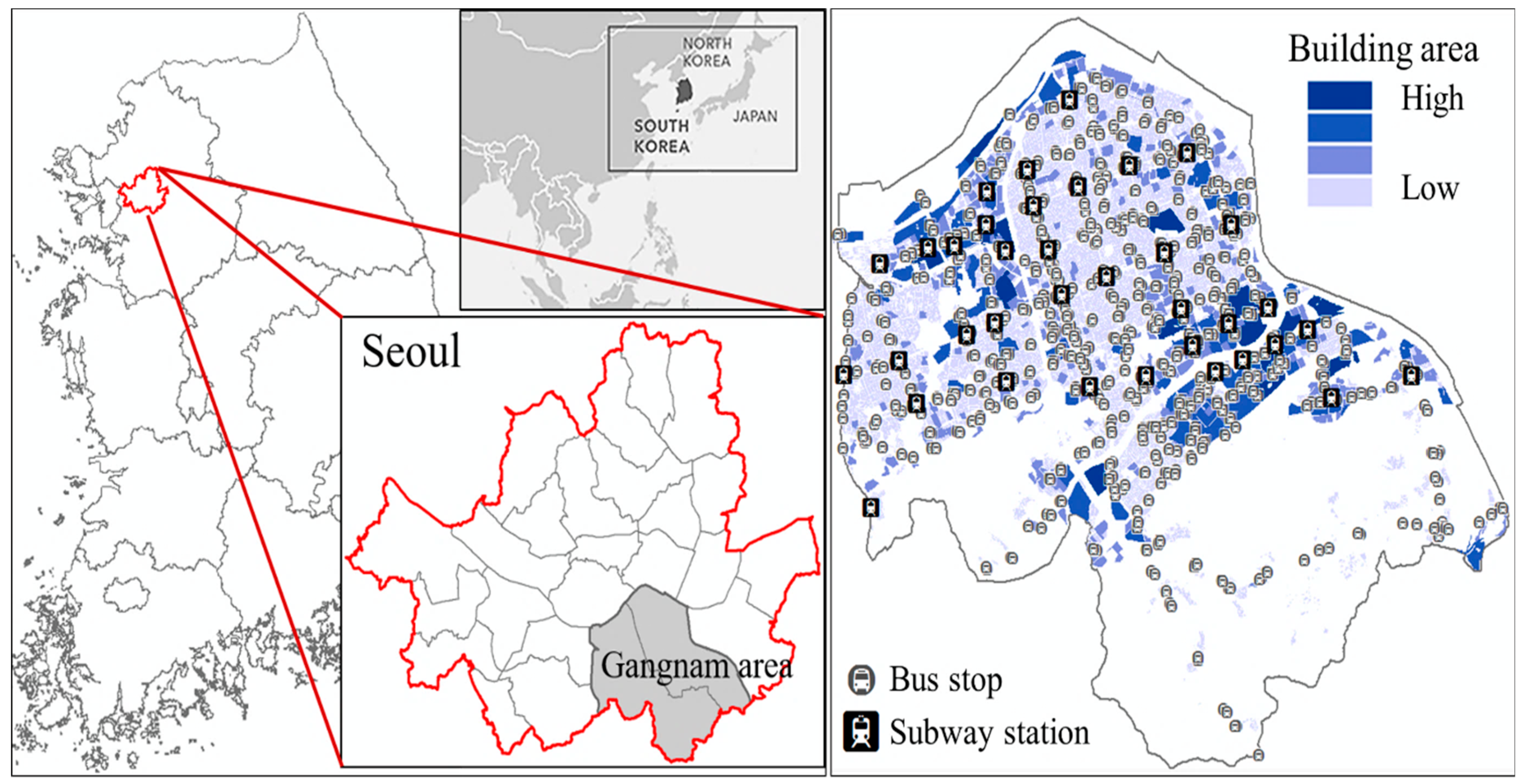
Figure 1. Target area for analysis.
Sustainability 15 04407 g001
Figure 2. Traffic volume and land use area by zone.
Sustainability 15 04407 g002
Figure 3. Multi-objective trips produced and attracted by each building ('*' is one building in the target area).
Sustainability 15 04407 g003
Figure 4. Average modal share rates of each trip type in the Gangnam area.
Sustainability 15 04407 g004
Figure 5. Modal share rate of each trip type for each building. ('*' is one building in the target area).
Sustainability 15 04407 g005
Figure 6. Origin and destination selection area for each mode. ('*' is one building in the target area).
Sustainability 15 04407 g006
Figure 7. Transit ridership of each public transport node.
Sustainability 15 04407 g007
Figure 8. Bus users assigned to the network. ('*' is one building in the target area).
Sustainability 15 04407 g008
Figure 9. Subway users assigned to the network. ('*' is one building in the target area).
Sustainability 15 04407 g009
Figure 10. Destination choice characteristics of foot passengers for each traffic purpose.
Sustainability 15 04407 g010
Figure 11. Network area by each distance unit. ('*' is one building in the target area).
Sustainability 15 04407 g011
Figure 12. Calculated results for the walking traffic in a cell. ('*' is one building in the target area).
Sustainability 15 04407 g012
Figure 13. Simple conceptual diagram of the calculation method at each point.
Sustainability 15 04407 g013
Figure 14. Observed and estimated pedestrian volumes at each survey point.
Sustainability 15 04407 g014
Figure 15. Comparison between the observed and estimated pedestrians for each point.
Sustainability 15 04407 g015
Figure 16. Difference between the observed and estimated pedestrians in Gangnam.
Sustainability 15 04407 g016
Table 1. Home-based trip production model.
Independent Variable HBW _ P   R 2 :0.465 HBS _ P   R 2 :0.578 HBO _ P   R 2 :0.211
BβBβBβ
Constant−12,944.601- −2007.918- 127.186-
Land useDetached house0.0080.198***0.0060.223***0.0020.282***
Multihouse-- 0.0370.071**- -
Multihousehold house0.0100.186***0.0030.095**- -
Official residence−0.4890.186***−0.243−0.067**- -
Apartment0.0050.607**0.0030.567***0.0010.504***
Multiplex house0.0100.257***0.0050.216***--
Row house- --- 0.0020.122***
Dormitory0.0970.090***-- --
SocioeconomicPop 10–19%- -275.9660.437***--
Pop 20–34%168.3360.362**-- 7.6900.110**
Pop 35–49%373.2660.339***-- --
Pop 50–64%151.4830.129**-- --
Land price0.000−0.217***-- --
***: p < 0.01; **: p < 0.05.
Table 2. Home-based trip attraction and non-home-based trip models.
Independent Variable HBW _ A   R 2 :0.979 HBS _ A   R 2 :0.524 HBO _ A   R 2 :0.576 NHB _ P   R 2 :0.476 NHB _ A   R 2 :0.781
BβBβBβBβBβ
Constant829.704- 259.284- 338.108- 216.532- 155.062-
Land useType-1 neighborhood living0.0230.129***-- 0.0020.186***0.0020.313***0.0010.104***
Type-2 neighborhood living0.0150.102***-- -- -- --
Cultural assembly0.0210.034***-- -- 0.0030.162***0.0050.119***
Religious-- -- 0.0080.114***0.0040.080**--
Transportation0.0200.046***-- -- -- --
Medical0.0120.028***-- 0.0040.173***-- --
Education and research0.0060.030***0.0180.420***0.0020.180***-- 0.0010.101***
Training-- -- 0.0530.123***0.0230.076**0.0380.067***
Sports-- 0.0250.093***-- -- --
Office0.0370.714***-- 0.0010.371***0.0000.248***0.0020.672***
Accommodations-- -- -- -- 0.0030.074**
Recreational0.0740.036***-- 0.0190.194***0.0080.120***0.0100.079***
Factory0.0180.252***-- -- -- 0.0010.219***
Automobile-related−0.016−0.060***-- −0.002−0.152***-- −0.002−0.137***
Correctional or military-- -- -- -- 0.0190.089***
Communication−0.089−0.069***-- -- −0.005−0.119***--
Power-- -- -- −0.116−0.203***−0.083−0.077**
Temporary building-- -- 1.3960.106***-- --
Neighborhood living0.0200.088***-- 0.0010.090**0.0020.274***0.0020.143***
Sales and business0.0420.070***-- 0.0020.087**-- --
Education and research or welfare-- 0.0180.124***-- -- --
Public-- -- -- -- −0.011−0.092***
SocioeconomicConstruction %−49.490−0.023**-- -- -- --
Accommodation or restaurant %−98.128−0.036***-- -- -- --
Publishing or video and broadcasting communication and information %179.7790.061***-- -- -- --
Elementary %-- 120.6400.143***-- -- --
Middle %-- 240.5440.184***-- -- --
High %-- 46.7140.338***-- -- --
University or higher %-- 40.2600.314***-- -- --
***: p < 0.01; **: p < 0.05.
Disclaimer/Publisher’s Note: The statements, opinions and data contained in all publications are solely those of the individual author(s) and contributor(s) and not of MDPI and/or the editor(s). MDPI and/or the editor(s) disclaim responsibility for any injury to people or property resulting from any ideas, methods, instructions or products referred to in the content.