Identifying the PEM Fuel Cell Parameters Using Artificial Rabbits Optimization Algorithm

Abstract

The artificial rabbits optimization (ARO) algorithm is proposed in this article to find the optimum values for uncertain parameters for the proton exchange membrane fuel cell (PEMFC) model. The voltage–current polarization curve of the PEMFC is nonlinear, and the model used in this paper to describe it is Mann’s model, which has seven uncertain parameters. The sum of square errors (SSE) between the ARO-based estimated voltages of the model and the measured voltages of the fuel cell defines the objective function. The simulation results show that the ARO technique has the best SSE compared to other optimization techniques. The precision of the ARO model is evaluated by comparing the optimized model’s power–current and voltage–current curves with the measured curves of three stacks which are NedStack PS6, BCS stack 500 W, and Ballard Mark V. The results show that the estimated curves and measured curves are very close which, means a high accuracy is achieved. Moreover, the ARO method shows a fast convergence curve with a minimal standard deviation. Furthermore, the PEMFC-optimized model is studied at different temperature and pressure operating conditions.

1. Introduction

Due to the decrease of fossil fuels worldwide and their impact on the environment, the need for clean, renewable, and continuous energy sources increases every day [1]. However, the power generation from renewable energy sources such as wind and solar energy is intermittent as they depend on weather conditions, location, and time [2]. Fuel cells do not have this problem as they produce electrical power as long as they are supplied with sufficient fuel. One of its types is the proton exchange membrane fuel cell (PEMFC) which uses the chemical reaction of oxygen and hydrogen gases to produce water and electrical energy [3,4]. Not only is the PEMFC a clean source of energy; it also has high efficiency (30–60%), no waste material, high reliability, fast startup, lightweight, and low operating temperature and pressure [4,5,6]. However, the PEMFC has some disadvantages: it needs an expensive metal catalyst, is highly sensitive to carbon monoxide, and needs complex water and thermal management [7]. Moreover, the electrolyte membranes of PEMFC suffer from a decrease in proton conductivity as the environment’s relative humidity decreases or the temperature rises [8]. The PEMFC is used in many applications such as micro-combined heat and power applications [9,10], microgrid applications [11], and domestic applications [12]. It is also used in feeding switched reluctance motors [13,14] and in power systems as distributed generation [15]. Other fuel cell types, such as alkaline fuel cells (AFC), molten carbonate fuel cells (MCFC), phosphoric acid fuel cells (PAFC), and solid oxide fuel cells (SOFC), are categorized based on the electrolyte used [7,16].

The voltage–current characteristics of PEMFC are nonlinear and depend on the operating conditions (temperature and pressure) [3], so obtaining an accurate model of PEMFC became the focus of many researchers [17].

From the models used to describe the PEMFC performance is Mann’s model, a semi-empirical model that has seven unknown parameters [18]. Extracting the parameters of the PEMFC became necessary as the model’s accuracy depended on it. It can be accomplished using either meta-heuristic optimization algorithms or conventional analytical methods. The stochastic method [19], the input-output diffusive approach [20], and the proper generalized decomposition approach [21] are from the conventional methods used. Geem and others [22] used the generalized reduced gradient method. However, such methods have many demerits, such as their dependence on the problem’s initial conditions, the probability of being trapped into a local minimum point, and their accuracy depending on the differential equations’ solver error [5].

For the reasons mentioned above, many researchers focused on using meta-heuristic algorithms as they have no restrictions on the problem formulation, are derivative-free, and can be used with various real engineering problems [23]. Many meta-heuristic algorithms were used to obtain the best values of the uncertain parameters, such as the mayfly optimization algorithm [1], marine predator algorithm [3], chaotic harris hawks optimization [4], manta rays foraging optimizer [5], and Jellyfish search algorithm [6]. EL-Fergany and others used a grasshopper optimizer [16], a whale optimization algorithm [17], and a salp swarm optimizer [24]. In [25], Seleem and others used the equilibrium optimizer. Moreover, the chaos game optimization technique was used by Alsaidan [26]. Sultan and others [27] identified the fuel cell parameters utilizing improved chaotic electromagnetic field optimization. Furthermore, the artificial ecosystem optimizer was used in [28]. Rao and others [29] applied a shark smell optimizer to the PEMFC model, while Fahim and others [30] utilized the hunger games search algorithm. Ref. [31] used a novel circle search algorithm. Ali and others [32] proposed a grey wolf optimizer (GWO) to obtain the optimal PEMFC parameters. Abaza and others [33] introduced a coyote optimization algorithm (COA) for solving the PEMFC problem, while Zaki and others [34] used marine predators and political optimizers. Chen and others [35] utilized a cuckoo search algorithm (CS). In addition, Kandidayeni and others [36] used the firefly optimization algorithm (FOA) and shuffled frog leaping algorithm (SFLA) to model the PEMFC. Niu and others [37] applied the biogeography-based optimization algorithm (BBO) to find the parameters of the fuel cell. Askazrzadeh and others used a backtracking search algorithm (BSA) [38], a bird mating optimizer (BMO) [39], and a grouping-based global harmony search algorithm (GGHS) [40]. In [41], Chakraborty and others used differential evolution (DE) to find the PEMFC parameters, while Priya and others [42] utilized a flower pollination algorithm (FPA). Outeiro and others used the simulated annealing optimization algorithm (SA) in [43].

Most algorithms above have long computational steps, and their procedure is complex [44]. Moreover, due to the nonlinear nature of the characteristics of PEMFC, most of the meta-heuristic algorithms show some drawbacks. Some of these techniques have premature convergence, such as CS [35], FOA [36], and BBO [37]. Other techniques have low convergence speeds, such as GWO [32], SFLA [36], BSA [38], and DE [41]. Moreover, some techniques require complex parameter settings and tunings, such as FPA [42], BMO [39], and SA [43]. In addition, some algorithms are easily trapped at a local optimum solution, such as CS [35] and GGHS [40]. Although they have some drawbacks, they also have advantages. GWO and COA have simple tuning variables. Moreover, the Jellyfish search optimizer, Shark smell optimizer, and Neural network optimizer are distinguished by low computational efforts. In addition, the COA, Marine predator optimizer, and Equilibrium optimizer have a high convergence speed [45].

For the reasons mentioned above and to gain a more accurate model, a new technique known as the Artificial Rabbits optimization algorithm (ARO) is suggested to solve the PEMFC model. Wang and others first introduced it in [46]. It is based on a random hiding strategy and the detour foraging strategy that the rabbits use to survive in nature [46].

This paper’s primary contributions are:

• The Ballard Mark V stack, the BSC 500 W stack, and the NedStack PS6 are the three stacks for which the ARO is used to determine the optimal values for the seven uncertain PEMFC model parameters;
• The results of ARO are compared to various algorithms such as manta rays foraging optimizer (MRFO), salp swarm optimizer (SSO), whale optimization algorithm (WOA), jellyfish search algorithm (JSA), grasshopper optimizer algorithm (GOA), circle search algorithm (CSA) and enhanced transient search optimization (ETSO);
• The optimized model’s P-I and V-I curves are compared with the three stacks’ measured curves.

This article has five sections: Section 1 is the introduction. Section 2 illustrates the description of the problem and the PEMFC model to be optimized. The ARO algorithm is illustrated in Section 3. Discussion of the simulation findings and comparisons is included in Section 4, and Section 5 contains the conclusion.

2. Problem Description

2.1. PEMFC Principle of Operation

As mentioned, PEMFC converts chemical energy from hydrogen and oxygen gas reactions into water and electrical energy. It consists of a cathode, anode, and a proton exchange membrane separating them, which acts as an electrolyte. The hydrogen (fuel) ionizes at the anode and forms electrons and protons. The membrane allows the protons to go to the cathode through it but prevents the electrons from passing; thus, through an external circuit, the electrons travel to the cathode. The oxygen reacts with the electrons and protons at the cathode, producing water.

$$\mathrm{Anode}:2{\mathrm{H}}_2\to 4{\mathrm{H}}^{+}+4{\mathrm{e}}^{-}$$

(1)

$$\mathrm{Cathode}:{\mathrm{O}}_2+4{\mathrm{e}}^{-}+4{\mathrm{H}}^{+}\to 2{\mathrm{H}}_2\mathrm{O}+\mathrm{energy}$$

(2)

2.2. PEMFC Model

The I-V polarization curve of the PEMFC has three types of voltage drops which can be summed up as follows:

• The energy required to start the chemical reaction is the activation voltage drop;
• The energy lost in the resistance of the contacts, membrane, and electrodes is the ohmic voltage drop;
• The concentration voltage drop is losses that happen because the oxygen and hydrogen consumption rate is higher than the rate of their supply at a high current density, which causes their concentration to decrease.

The PEMFC stack has many cells connected in series, and its total output voltage (V_Stack) is calculated using Equations (3)–(11), as in [3,31].

$${\mathrm{V}}_{\mathrm{Stack}}={\mathrm{N}}_{\mathrm{c}}\left({\mathrm{E}}_{\mathrm{Nernst}}-{\mathrm{V}}_{\mathrm{act}}-{\mathrm{V}}_{\mathrm{ohm}}-{\mathrm{V}}_{\mathrm{con}}\right)$$

(3)

where V_Stack is the output voltage of the stack, N_c is the number of cells in the stack, V_act is the activation voltage drop per cell, V_ohm is the ohmic voltage drop per cell, V_con is the concentration voltage drop per cell, and E_Nernst is the Nernst voltage per cell. It is calculated for operating temperatures under 100 °C using Equation (4), as follows:

$$\begin{array}{l}{\mathrm{E}}_{\mathrm{Nernst}}=1.229-0.85\times {10}^{-3}\left({\mathrm{T}}_{\mathrm{FC}}-298.15\right)\\ \hspace{1em}\hspace{1em}\hspace{1em}\hspace{1em}\hspace{1em}\hspace{1em}\hspace{1em}+4.3085\times {10}^{-5}{\mathrm{T}}_{\mathrm{FC}}\ln \left({\mathrm{P}}_{{\mathrm{H}}_2}\sqrt{{\mathrm{P}}_{{\mathrm{O}}_2}}\right)\end{array}$$

(4)

where T_FC is the fuel cell operating temperature in (Kelvin), and P_O2 and P_H2 are the oxygen and hydrogen partial pressures in (atm), respectively. The activation voltage drop V_act can be represented as:

$${\mathrm{V}}_{\mathrm{act}}=-\left[{\mathsf{\xi }}_1+{\mathsf{\xi }}_2{\mathrm{T}}_{\mathrm{FC}}+{\mathsf{\xi }}_3+{\mathrm{T}}_{\mathrm{FC}}\ln \left({\mathrm{C}}_{{\mathrm{O}}_2}\right)+{\mathsf{\xi }}_4{\mathrm{T}}_{\mathrm{FC}}\ln \left({\mathrm{I}}_{\mathrm{FC}}\right)\right]$$

(5)

$${\mathrm{C}}_{{\mathrm{O}}_2}=\left(\frac{{\mathrm{P}}_{{\mathrm{O}}_2}}{5.08\times {10}^6}\right){\mathrm{e}}^{\frac{498}{{\mathrm{T}}_{\mathrm{FC}}}}$$

(6)

where ξ₁, ξ₂, ξ₃, ξ₄ are semi-empirical coefficients, I_FC is the current of the stack in (Ampere), and ${\mathrm{C}}_{{\mathrm{O}}_2}$ is the oxygen concentration in (mol·cm⁻³). Moreover, the ohmic voltage drop is determined as follows:

$${\mathrm{V}}_{\mathrm{ohm}}={\mathrm{I}}_{\mathrm{FC}}(\mathrm{Rm}+\mathrm{Rc})$$

(7)

$$\mathrm{Rm}=\frac{{\mathsf{\rho }}_{\mathrm{m}}{\mathrm{L}}_{\mathrm{m}}}{\mathrm{A}}$$

(8)

$${\mathsf{\rho }}_{\mathrm{m}}=\frac{181.6[1+0.03\mathrm{J}+0.062{\left(\frac{{\mathrm{T}}_{\mathrm{FC}}}{303}\right)}^2\times {\mathrm{J}}^{2.5}]}{\left[\mathsf{\lambda }-0.634-3\mathrm{J}\right]{\mathrm{e}}^{4.18(1-\frac{303}{{\mathrm{T}}_{\mathrm{FC}}})}}$$

(9)

$$\mathrm{J}=\frac{{\mathrm{I}}_{\mathrm{FC}}}{\mathrm{A}}$$

(10)

where Rc and Rm are the resistance of the connections and membrane, respectively. A, L_m, ρ_m, and J are the surface area of the membrane in (cm²), the membrane thickness in (cm), membrane specific resistance in (ohm·cm), and current density in (A/cm²), respectively. λ is an adjustable parameter.

Finally, the concentration voltage drop is calculated as follows:

$${\mathrm{V}}_{\mathrm{con}}=-\mathsf{\beta }\ln \left(1-\frac{\mathrm{J}}{{\mathrm{J}}_{\max }}\right)$$

(11)

where β represents an adjustable coefficient, and J_max is the max current density.

2.3. Problem Formulation

The model above has seven uncertain parameters due to the lack of data given by the manufacturer, which are ξ₁, ξ₂, ξ₃, ξ₄, λ, Rc, and β, whose ranges are given in the previous literature [3], as shown in Table 1. Hence, the artificial rabbit optimizer is used to optimize the value of previously mentioned parameters such that the square difference between the experimentally measured voltage values matches the calculated voltage values from the model equation and can be represented by the following Equation (12):

$$\mathrm{SSE}={\displaystyle \sum }_{\mathrm{i}=1}^{\mathrm{N}}{\left({\mathrm{V}}_{\mathrm{meas}}\left(\mathrm{i}\right)-{\mathrm{V}}_{\mathrm{est}}\left(\mathrm{i}\right)\right)}^2$$

(12)

where N represents the number of measured voltage samples.

Table 1. PEMFC parameters constraints.

Parameters	ξ1	ξ2	ξ3	ξ4	λ	Rc	β
Max Value	−0.8532	0.005	9.8 × 10−5	−9.5 × 10−5	24	0.0008	0.5
Min Value	−1.1997	0.001	3.6 × 10−5	−2.6 × 10−4	10	0.0001	0.0136

3. Artificial Rabbits Optimization (ARO)

The survival strategies used by rabbits in nature served as an inspiration for the ARO algorithm. Rabbits look for food away from their nests, which is called the detour foraging strategy. To escape from hunters and predators, they make burrows around their nests and randomly hide in one of them; this is called the random hiding strategy. They will choose to do either detour foraging or random hiding based on their energy. When they have high or sufficient energy, they will search for food at locations far away from their nests (detour foraging), and when they have low energy, they will randomly hide in the near burrows around their nests. Section 3.1, Section 3.2 and Section 3.3 provides the steps and the equations used to update the rabbits’ positions, which can be summarized in Figure 1. For more details, check [46].

Figure 1. Artificial rabbits optimization algorithm flowchart.

3.1. Energy Shrink (Switch between Exploration and Exploitation)

Rabbits choose to do either random hiding or detour foraging. This depends on the amount of energy a rabbit has, so an energy factor A(t) is calculated according to Equation (13) to simulate which one the rabbit will do. When A(t) > 1, a rabbit will do detour foraging, and when A(t) ≤ 1, it will do random hiding.

$$A\left(t\right)=4\left(1-\frac{t}{T}\right)\ln \frac{1}{r}$$

(13)

where r is a number chosen at random between (0,1).

3.2. Detour Foraging (Exploration)

Rabbits search for food away from their nests, thus protecting their nests from predators. Equation (14) indicates that rabbits search randomly for food according to each other’s position.

$$\begin{array}{l}{\overrightarrow{p}}_i\left(t+1\right)={\overrightarrow{x}}_j\left(t\right)+R\times \left({\overrightarrow{x}}_i\left(t\right)-{\overrightarrow{x}}_j\left(t\right)\right)+round\left(0.5\times \left(0.05+r_1\right)\right)\times n_1,i,j\\ \hspace{1em}\hspace{1em}\hspace{1em}\hspace{1em}\hspace{1em}\hspace{1em}\hspace{1em}\hspace{1em}=1,\dots ,n\mathrm{and}j\ne i\end{array}$$

(14)

$$R=L\times c$$

(15)

$$L=(e-e^{{\left(\frac{t-1}{T}\right)}^2}\times sin\left(2\pi r_2\right)$$

(16)

$$c\left(k\right)=\{\begin{array}{c}1 if k=g\left(l\right)\\ 0 else \end{array} k=1,\dots ,d\mathrm{and}l=1,\dots ,\left[r_3·d \right]$$

(17)

$$g=rand perm\left(d\right)$$

(18)

$$n_1 ~ N\left(0,1\right)$$

(19)

where ${\overrightarrow{p}}_i\left(t+1\right)$ is the candidate’s position of ith rabbit at the time t + 1, while ${\overrightarrow{x}}_i\left(t\right)$ is the ith rabbit’s position at the time t, n is the rabbit’s population size, d is the number of variables in the problem that needs to be optimized, T is the maximum number of iterations, L represents the movement pace of rabbits, r₁, r₂, and r₃ are three random numbers between (0,1) and n₁ is subject to the standard normal distribution. c is a mapping vector, while R represents the running operator that simulates rabbits’ running characteristics.

3.3. Random Hiding (Exploitation)

Each rabbit has d burrows around its nest to select one of them randomly to hide in and escape from predators. These burrows are generated for each rabbit by Equation (20).

$${\overrightarrow{b}}_{i,j}\left(t\right)={\overrightarrow{x}}_i\left(t\right)+H\times g\times {\overrightarrow{x}}_i\left(t\right),i=1,\dots ,n\mathrm{and}j=1,\dots ,d$$

(20)

$$H=\frac{T-t+1}{T}\times r_4$$

(21)

$$g\left(k\right)=\{\begin{array}{c}1 if k=j\\ 0 else \end{array}k=1,\dots ,d$$

(22)

$${\overrightarrow{p}}_i\left(t+1\right)={\overrightarrow{x}}_i\left(t\right)+R\times \left(r_4\times {\overrightarrow{b}}_{i,r}\left(t\right)-{\overrightarrow{x}}_i\left(t\right)\right)i=1,\dots ,n$$

(23)

$$g_r\left(k\right)=\{\begin{array}{c}1 if k=\left[r_5\times d\right]\\ 0 else \end{array}k=1,\dots ,d$$

(24)

$${\overrightarrow{b}}_{i,r}\left(t\right)={\overrightarrow{x}}_i\left(t\right)+H\times g_r\times {\overrightarrow{x}}_i\left(t\right),i=1,\dots ,n$$

(25)

$${\overrightarrow{x}}_i\left(t+1\right)=\{\begin{array}{c}{\overrightarrow{x}}_i\left(t\right) f({\overrightarrow{x}}_i\left(t\right))\le f({\overrightarrow{p}}_i\left(t+1\right))\\ {\overrightarrow{p}}_i\left(t+1\right) f({\overrightarrow{x}}_i\left(t\right))>f({\overrightarrow{p}}_i\left(t+1\right))\end{array}$$

(26)

where H is the hiding parameter, ${\overrightarrow{b}}_{i,j}$ is the jth burrow for the ith rabbit, ${\overrightarrow{b}}_{i,r}$ is a randomly selected burrow for hiding for the ith rabbit, shown in Equation (25), and r₄ and r₅ are random numbers between (0,1).

Equation (23) shows that the ith rabbit will attempt to change its position according to the randomly chosen burrow. At last, after either detour foraging or random hiding, the rabbit will leave the current position and remain at the candidate’s position if the fitness of the candidate’s position of ith rabbit is greater than that of the previous one, as shown by Equation (26).

4. Test Cases and Simulations Results

The performance of the ARO algorithm is validated in this section through three test cases: Ballard Mark V 5 kW, BSC 500 W, and NedStack PS6, and the algorithm’s results are compared with other techniques from previously published papers. The ARO parameters are population size = 50, max iterations = 2000, and it is implemented 20 times.

4.1. Test Case (1): Ballard Mark V

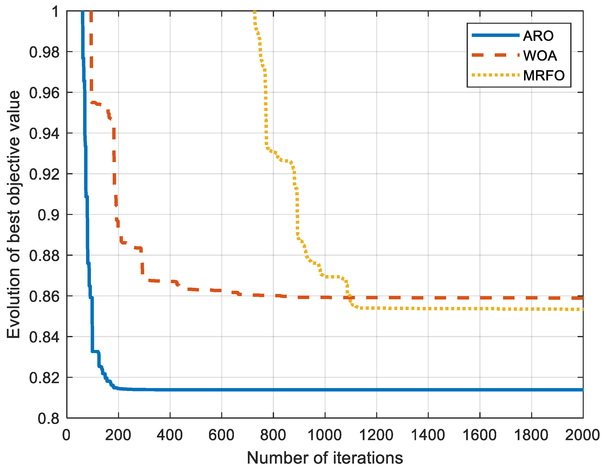
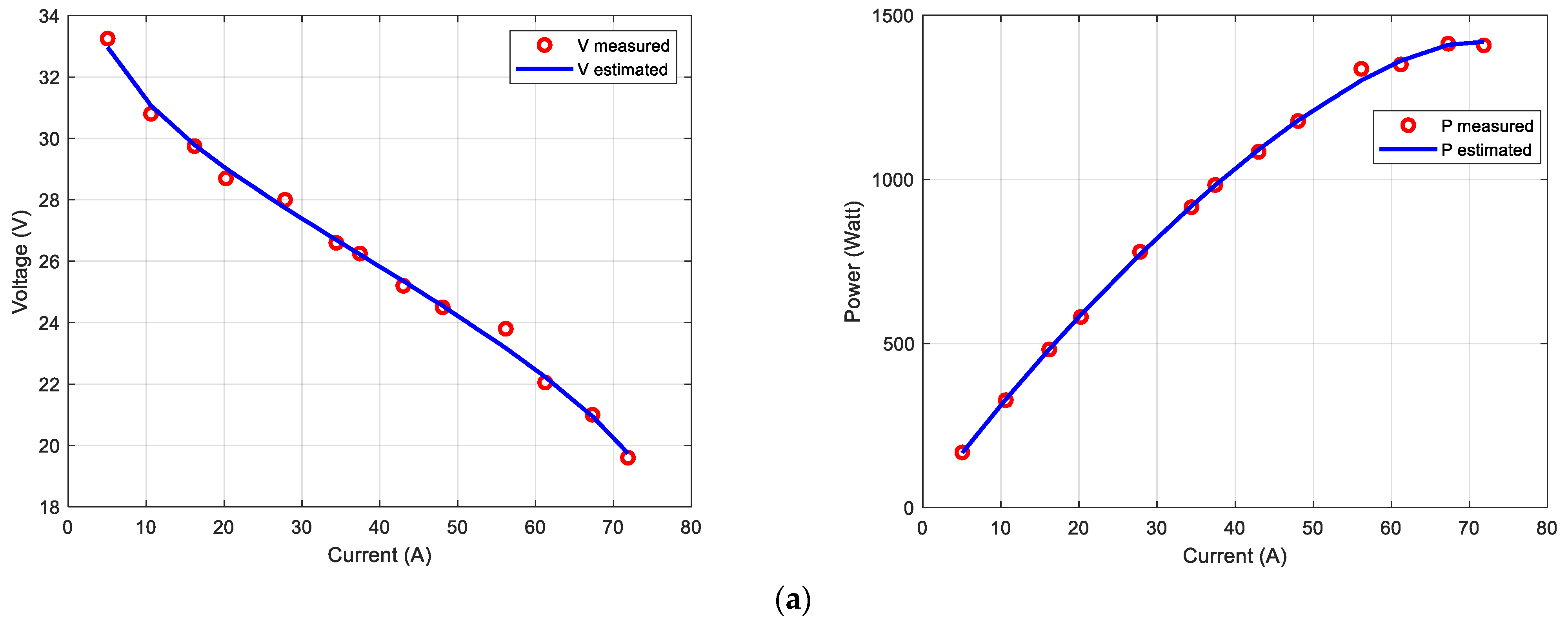
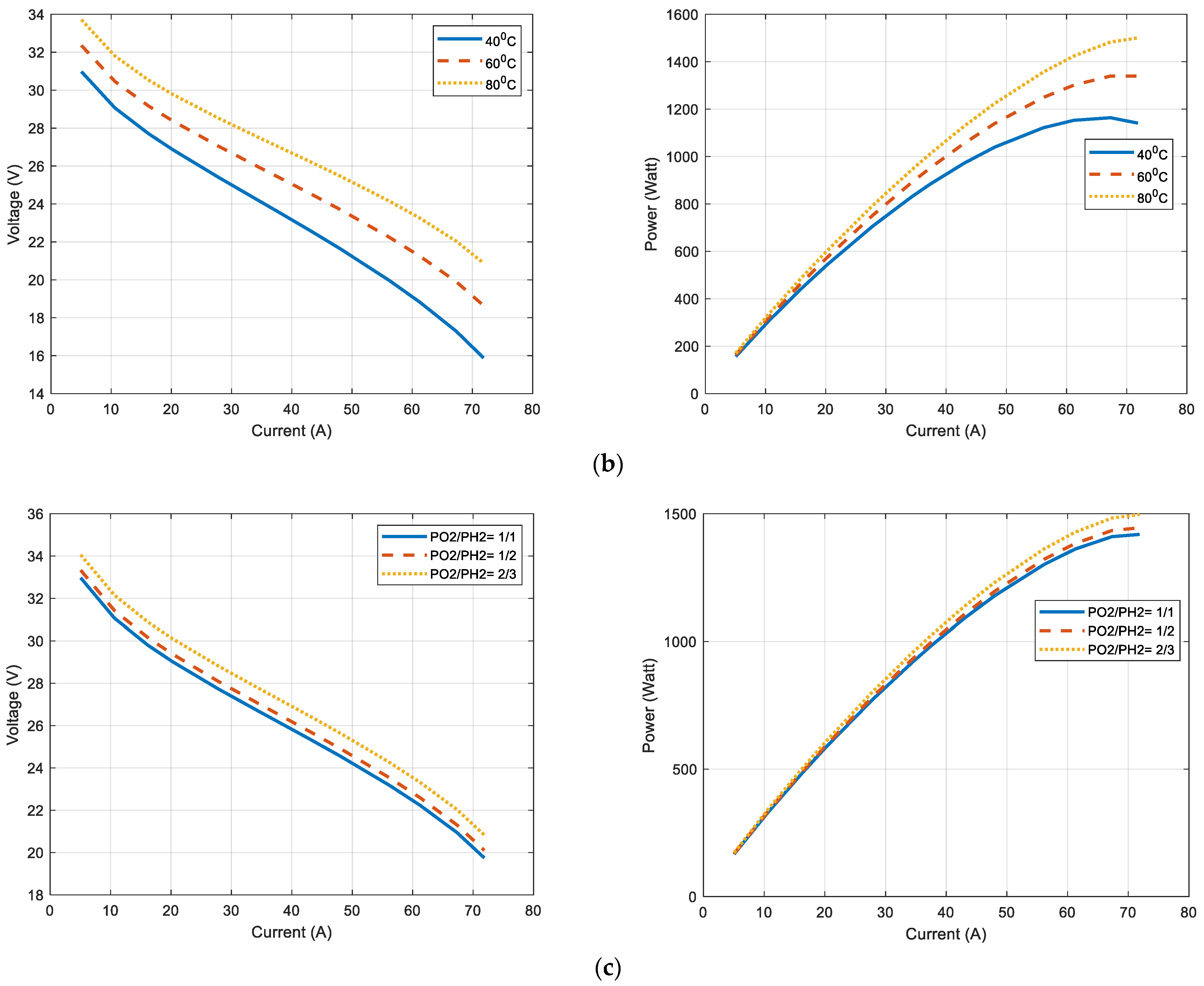
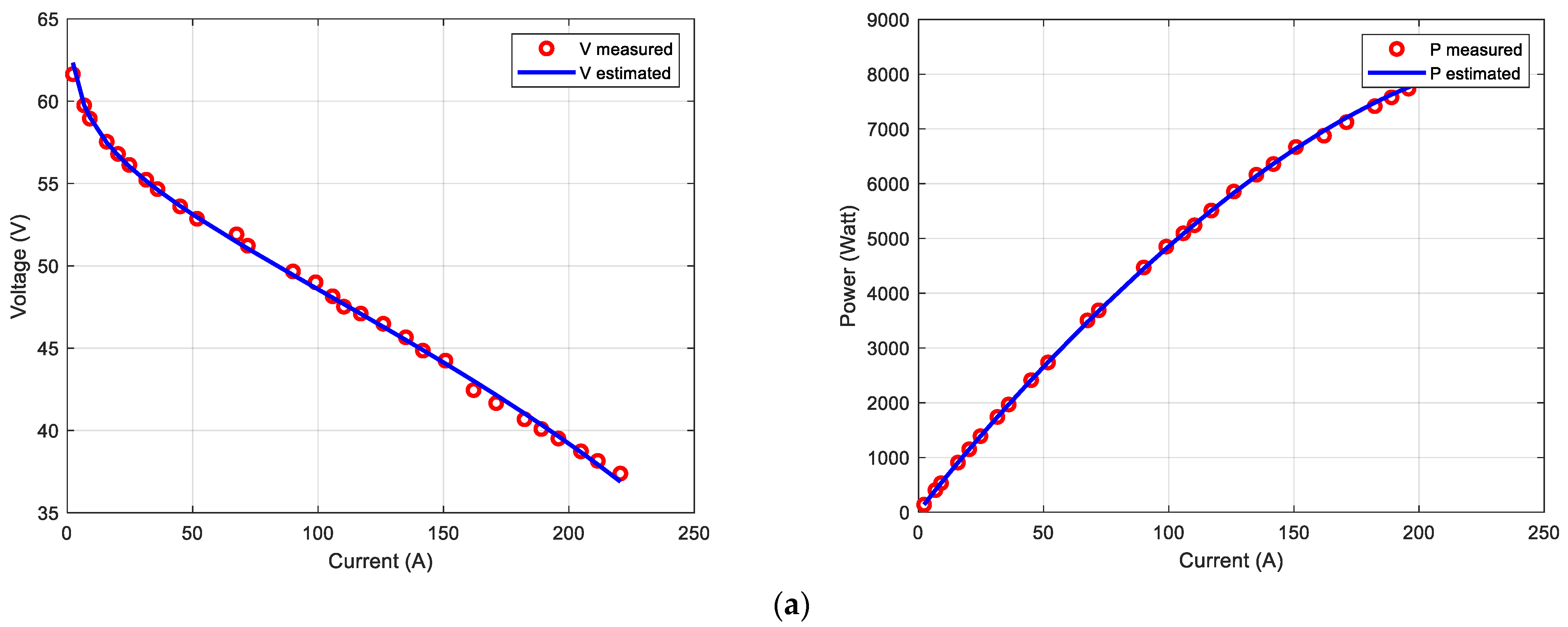
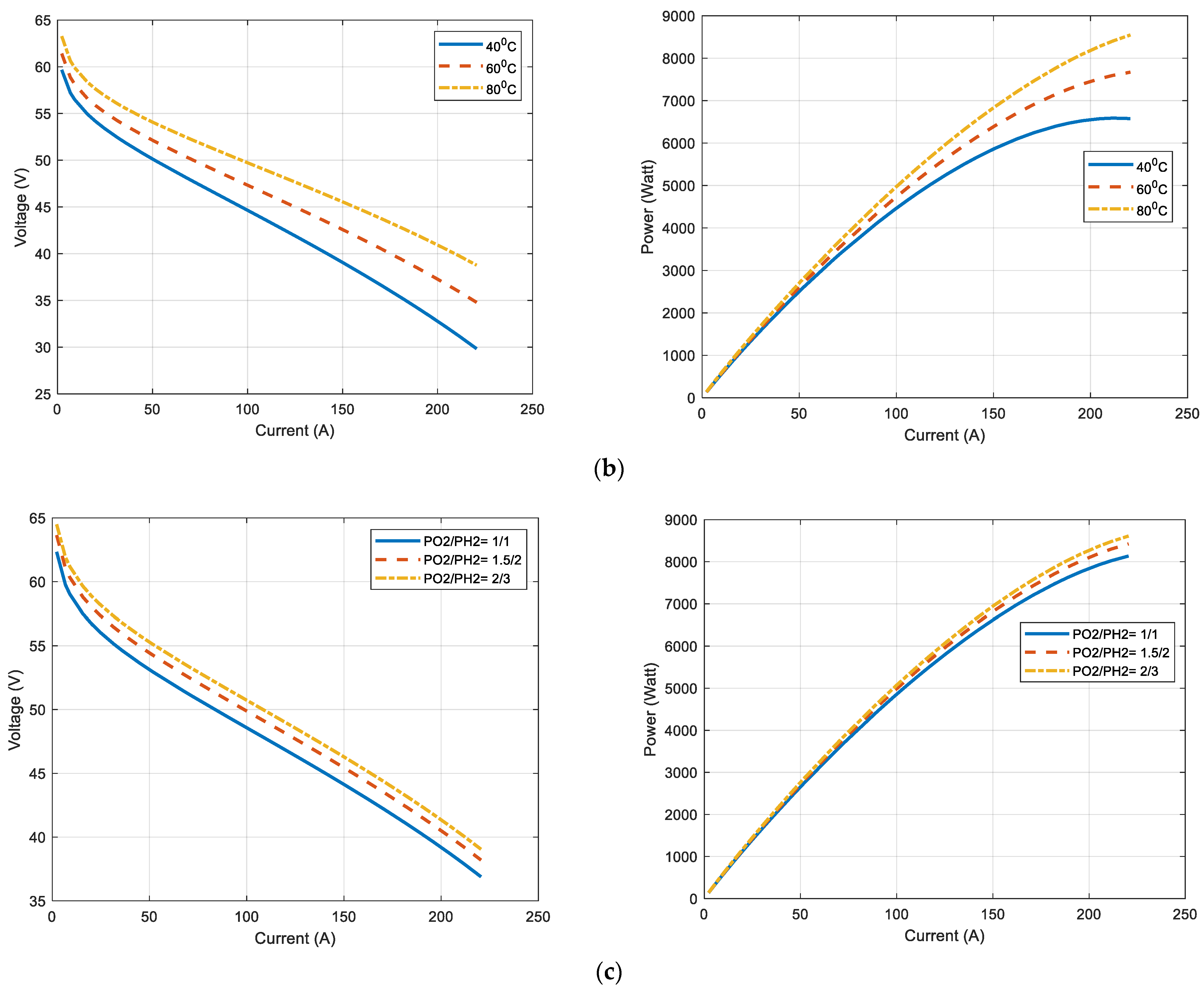
This stack has 35 cells with the thickness and surface area of the membrane of 178 µm and 50.6 cm², respectively. It has a maximum current density of 1.5 A/cm². Its experimental data from [5] and are given in Table 2. It was measured at a temperature of 70 °C and a pressure of 1 atm for both hydrogen and oxygen. Figure 2 shows the convergence curves of our proposed method ARO versus WOA and MRFO. It can be seen that the ARO method has the least SSE, and it converges steeper and faster than WOA and MRFO. The results of the optimized model (values of uncertain parameters) and SSE compared to other optimization techniques such as MRFO, WOA, CSA, ETSO, and neural network optimizer (NNO) are shown in Table 3. It is noted that the ARO technique has the least standard deviation, which means that it is more robust than the other algorithms. It is evident in Figure 3a that the optimized model’s computing power and voltage values are close to the measured values. Moreover, the effect of operating at different temperatures (40, 60, and 80 °C) and the effect of changing the ratios of partial pressures P_O2/P_H2 on the power and the voltage are presented in Figure 3b,c, respectively. It is shown in both figures that increasing the temperature or the pressure of hydrogen or oxygen or both leads to an increase in output voltage and power.

Table 2. Ballard Mark V measured and estimated voltages.

Im	Vm	Ve	${\left|{\mathbf{V}}_{\mathbf{m}}-{\mathbf{V}}_{\mathbf{e}}\right|}^2$
5.060	33.25	32.9678	0.0796
10.626	30.80	31.0685	0.0721
16.192	29.75	29.7941	0.0019
20.240	28.70	29.0203	0.1026
27.830	28.00	27.7316	0.0721
34.408	26.60	26.6930	0.0087
37.444	26.25	26.2217	0.0008
43.010	25.20	25.3538	0.0236
48.070	24.50	24.5456	0.0021
56.166	23.80	23.1730	0.3931
61.226	22.05	22.2323	0.0332
67.298	21.00	20.9511	0.0024
71.852	19.60	19.7474	0.0217
SSE			0.8139117035

Figure 2. Convergence curve of ARO, WOA, MRFO for Ballard Mark V.

Table 3. Results of the best PEMFC parameters and the corresponding SSE versus other techniques for Ballard Mark V.

Parameter	ARO	MRFO [5]	WOA [17]	CSA [31]	ETSO [44]	NNO [47]
ξ1	−1.158859	−1.0898	−1.1978	−1.181342	−0.853429	−0.97997
ξ2	3.5208 × 10−3	3.8249 × 10−3	4.4183 × 10−3	3.5691 × 10−3	2.5591 × 10−3	3.6946 × 10−3
ξ3	4.0526 × 10−5	7.7306 × 10−5	9.7214 × 10−5	3.9929 × 10−5	3.61 × 10−5	9.0871 × 10−5
ξ4	−16.7251 × 10−5	−16.283 × 10−5	−16.273 × 10−5	−16.283 × 10−5	−16.287 × 10−5	−16.282 × 10−5
λ	23.99	23	23	23	23	23
Rc	0.1 × 10−3	0.1 × 10−3	0.1002 × 10−3	0.1 × 10−3	0.1 × 10−3	0.1 × 10−3
β	0.015884	0.0136	0.0136	0.0136	0.0136	0.0136
SSE	0.8139117035	0.8533	0.8537	0.85360752	0.8536	0.8536
STD	2.706 e−14	0.0247	0.0239	2.29 e−6	0.020247	0.00854

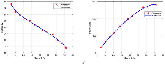
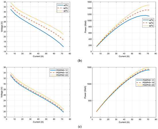
Figure 3. Polarization curves for Ballard Mark V: (a) estimated vs measured values; (b) under different temperatures; (c) under different partial pressures.

4.2. Test Case (2): BSC 500 W

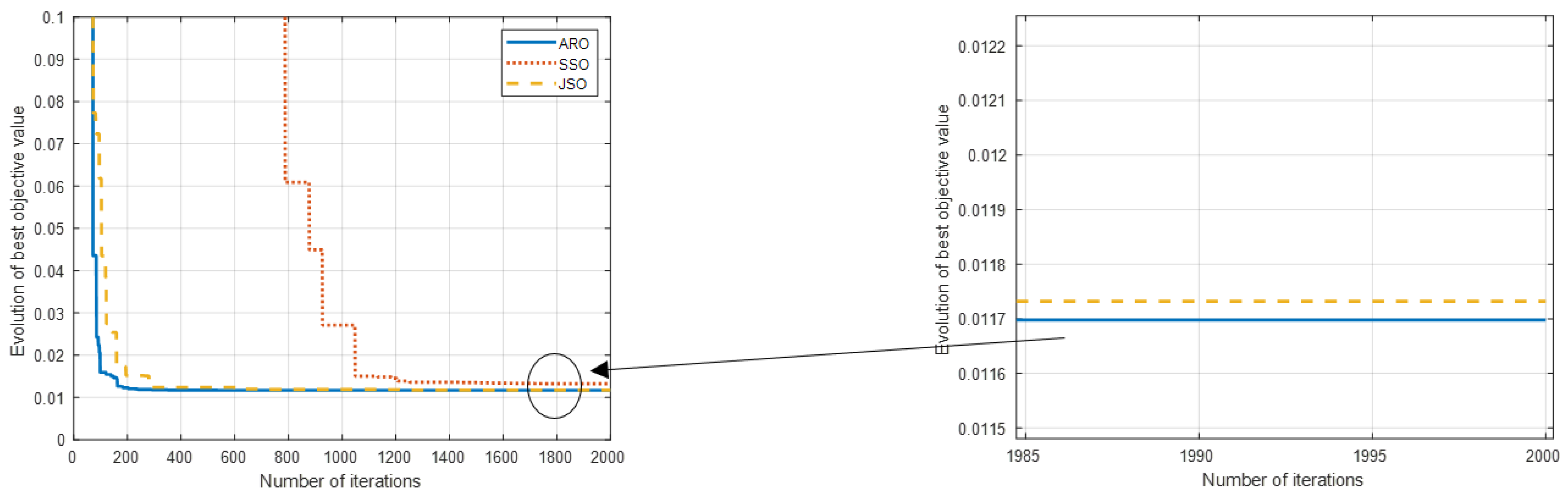
This stack has 32 cells with the thickness and surface area of the membrane of 178 µm and 64 cm², respectively. It has a maximum current density of 0.469 A/cm². Its experimental data are taken from [25] and presented in Table 4 and were measured at a temperature of 60 °C and a pressure of 1 atm and 0.2095 for hydrogen and oxygen, respectively. The convergence curves of ARO and other techniques are shown in Figure 4, and it shows that the ARO technique has a faster convergence curve than the other techniques. It can be noted from Table 5 that the ARO technique has lower SSE than SSO, CSA, and converged moth search algorithm (CMSA) and is very close to JSA but still better. Moreover, it shows that the ARO method has the least standard deviation, which means it is more robust. For more validation, the computing power and voltage values are shown against the measured values in Figure 5a. The model voltage and power curves are shown at different temperatures (40, 60, and 80 °C) in Figure 5b. Moreover, the model power and voltage curves under various partial pressure ratios P_O2/P_H2 are shown in Figure 5c. It is concluded from both figures that the output voltage and power increase with increasing temperature or pressure of hydrogen or oxygen or both.

Table 4. BSC 500 W measured and estimated voltages.

Im	Vm	Ve	${\left|{\mathbf{V}}_{\mathbf{m}}-{\mathbf{V}}_{\mathbf{e}}\right|}^2$
0.600	29.000	28.9972	0.00000771
2.100	26.310	26.3059	0.00001651
3.580	25.090	25.0936	0.00001264
5.080	24.250	24.2546	0.00002135
7.170	23.370	23.3754	0.00002933
9.550	22.570	22.5846	0.00021360
11.350	22.060	22.0713	0.00012831
12.540	21.750	21.7585	0.00007163
13.730	21.450	21.4613	0.00012685
15.730	21.090	20.9877	0.01045679
17.020	20.680	20.6945	0.00021052
19.110	20.220	20.2310	0.00012069
21.200	19.760	19.7709	0.00011976
23.000	19.360	19.3660	0.00003629
25.080	18.860	18.8665	0.00004181
27.170	18.270	18.2747	0.00002228
28.060	17.950	17.9533	0.00001096
29.260	17.300	17.2929	0.00005074
SSE			0.01169778

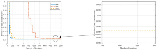
Figure 4. Convergence curve of ARO, SSO, JSO for BSC 500 W.

Table 5. Results of the best PEMFC parameters and the corresponding SSE versus other techniques for BSC 500 W.

Parameter	ARO	JSA [6]	SSO [24]	CSA [31]	CMSA [48]
ξ1	−1.176201	−0.96887	−0.8532	−1.176591	−0.785
ξ2	3.7344 × 10−3	2.693 × 10−3	4.8115 × 10−3	3.4965 × 10−3	4.5 × 10−3
ξ3	7.3729 × 10−5	4.67 × 10−5	9.4334 × 10−5	5.8319 × 10−5	8.86 × 10−5
ξ4	−19.3017 × 10−5	−19 × 10−5	−19.205 × 10−5	−19.2897 × 10−5	−19.3 × 10−5
λ	20.87724	20.8389	23	21.324206	23
Rc	0.1 × 10−3	0.1 × 10−3	0.3499 × 10−3	0.1464 × 10−3	0.312 × 10−3
β	0.016126	0.016111	0.01589	0.0161	0.017
SSE	0.01169778	0.011699	0.01219	0.0117362	0.012
STD	1.17746 × 10−8	1.66 × 10−4	8.711 × 10−4	2.34547 × 10−4	NR

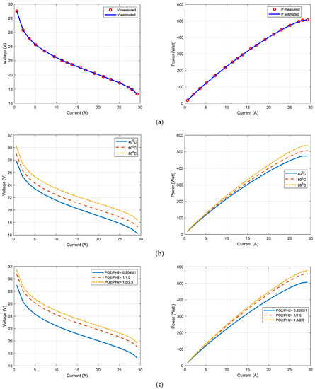
Figure 5. Polarization curves for BSC 500 W: (a) estimated vs measured values; (b) under different temperatures; (c) under different partial pressures.

4.3. Test Case (3): NedStack PS6

The rated power of NedStack PS6 is 6 kW. It has 65 cells with the thickness and surface area of the membrane of 178 µm and 240 cm², respectively. It has a maximum current density of 1.125 A/cm². Its experimental data are taken from [28] and given in Table 6 and measured at a temperature of 70 °C and a pressure of 1 atm for hydrogen and oxygen. The convergence curves of ARO and other techniques are presented in Figure 6. The convergence curve of the ARO technique is faster and smoother than that of the MRFO and grasshopper optimizer algorithm (GOA). The results of the optimized model compared to recently published techniques such as MRFO, GOA, vortex search algorithm (VSA), and balanced seagull optimization algorithm (BSOA) are shown in Table 7. It can be seen that the ARO technique has the least SSE and a minimal standard deviation. To show the precision of the optimized model, the calculated values of power and voltage are displayed against the measured values in Figure 7a. Moreover, Figure 7b illustrates the effect of operating at different temperatures (40, 60, and 80 °C) on the power and the voltage curves, while Figure 7c shows the effect of changing the ratios of partial pressures P_O2/P_H2 on the voltage and the power curves. It is clear that increasing the temperature or the pressure of hydrogen or oxygen or both increases the output voltage and power.

Table 6. NedStack PS6 measured and estimated voltages.

Im	Vm	Ve	${\left|{\mathbf{V}}_{\mathbf{m}}-{\mathbf{V}}_{\mathbf{e}}\right|}^2$
2.25	61.64	62.3350	0.4830
6.75	59.75	59.7633	0.0002
9.00	58.94	59.0332	0.0087
15.75	57.54	57.4846	0.0031
20.25	56.80	56.7084	0.0084
24.75	56.13	56.0376	0.0085
31.50	55.23	55.1542	0.0058
36.00	54.66	54.6200	0.0016
45.00	53.61	53.6374	0.0008
51.75	52.86	52.9521	0.0085
67.50	51.91	51.4562	0.2060
72.00	51.22	51.0460	0.0303
90.00	49.66	49.4465	0.0456
99.00	49.00	48.6596	0.1158
105.80	48.15	48.0666	0.0070
110.30	47.52	47.6739	0.0237
117.00	47.10	47.0877	0.0002
126.00	46.48	46.2954	0.0341
135.00	45.66	45.4946	0.0274
141.80	44.85	44.8822	0.0010
150.80	44.24	44.0597	0.0325
162.00	42.45	43.0134	0.3174
171.00	41.66	42.1509	0.2409
182.30	40.68	41.0353	0.1262
189.00	40.09	40.3542	0.0698
195.80	39.51	39.6460	0.0185
204.80	38.73	38.6788	0.0026
211.50	38.15	37.9337	0.0468
220.50	37.38	36.8931	0.2370
SSE			2.1112503

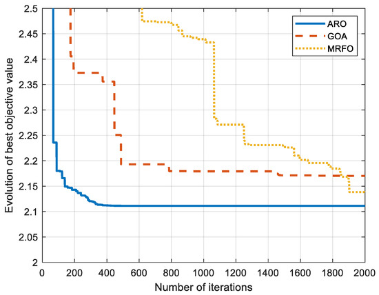
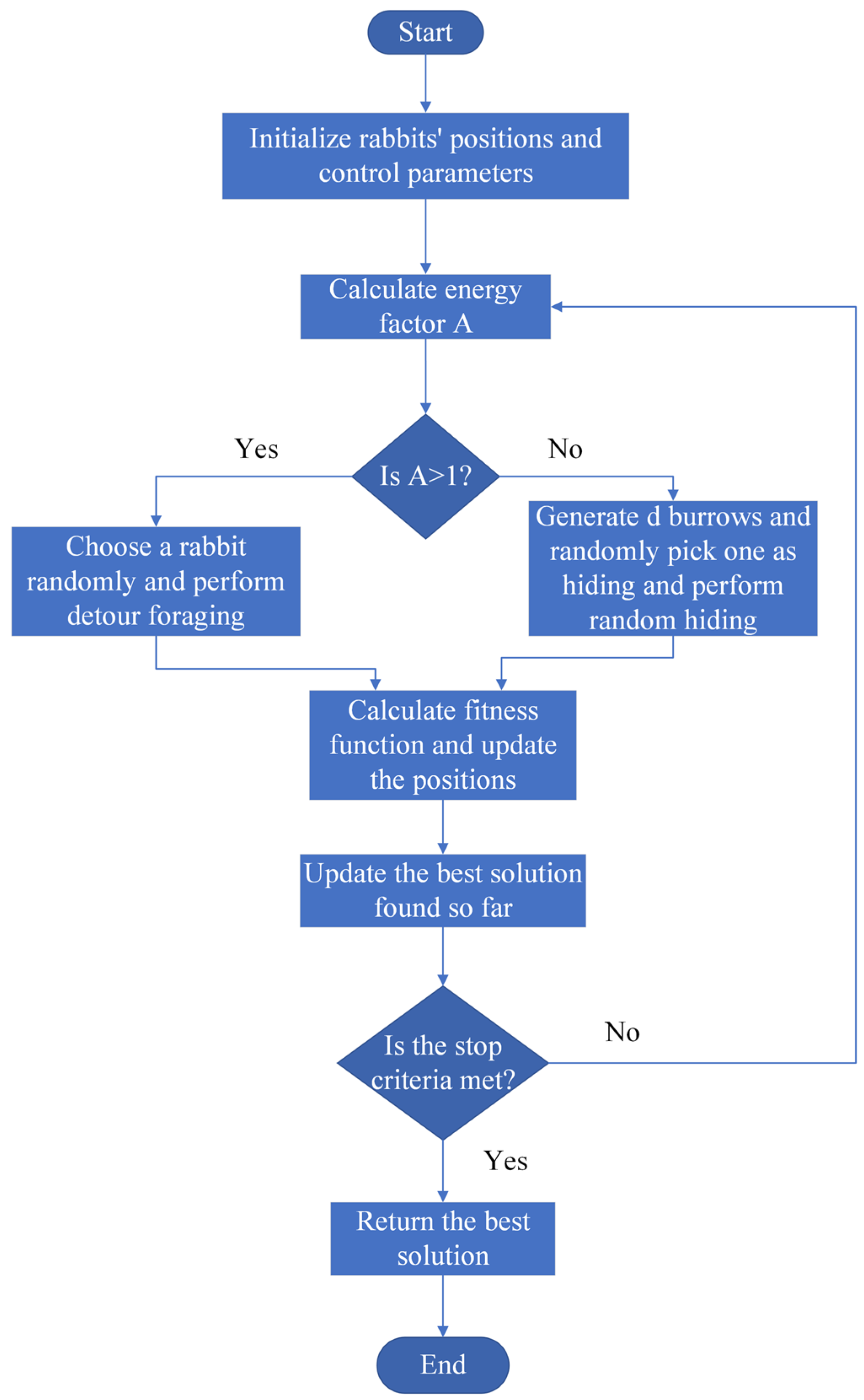
Figure 6. Convergence curve of ARO GOA, MRFO for NedStack PS6.

Table 7. Results of the best PEMFC parameters and the corresponding SSE versus other techniques for NedStack PS6.

Parameter	ARO	MRFO [5]	GOA [16]	VSA [49]	BSOA [50]
ξ1	−1.008511	−0.9381	−1.1997	−0.8946	−0.89
ξ2	3.0434 × 10−3	3.4861 × 10−3	3.5505 × 10−3	3.348 × 10−3	3.42 × 10−3
ξ3	4.9796 × 10−5	9.512 × 10−5	4.6144 × 10−5	9.75 × 10−5	7.76 × 10−5
ξ4	−9.54 × 10−5	−9.5436 × 10−5	−9.54 × 10−5	−9.54 × 10−5	−9.55 × 10−5
λ	13.445704	13.096	13.0092	13	13
Rc	0.1 × 10−3	0.1 × 10−3	0.1005 × 10−3	0.103 × 10−3	0.1 × 10−3
β	0.0136	0.014512	0.0579	0.0429	0.05
SSE	2.1112503	2.136	2.18586	2.3426	2.18
STD	4.6098 × 10−8	0.0326	NR	NR	NR

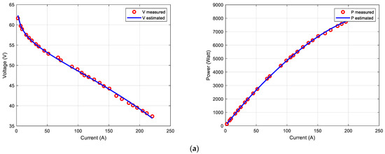
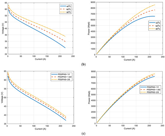
Figure 7. Polarization curves for NedStack PS6: (a) estimated vs measured values; (b) under different temperatures.; (c) under different partial pressures.

4.4. Sensitivity Analysis

This section will study the impact of altering the uncertain parameters on the SSE value. Table 8 shows the impact of altering the uncertain parameters by ±5%. It is found that the model is highly sensitive to ξ1 and ξ2 as the error increased by a significant value. The model is also moderately sensitive to ξ3, ξ4, and λ and less sensitive to Rc and β. It is concluded that any slight change from the ARO optimum values of the parameters will yield inaccurate results due to the model’s high nonlinearity.

Table 8. Sensitivity analysis.

Parameter	% Change	Ballard Mark V	BSC 500 W	NedStack PS6
		SSE	SSE	SSE
Best SSE		0.8139117035	0.01169781	2.1112503
ξ1	+5	54.28022983	63.76104277	313.66027116
	−5	54.28022987	63.76104242	313.66027172
ξ2	+5	58.87443251	71.26953933	335.90581476
	−5	58.87443248	71.29953969	335.90581477
ξ3	+5	2.319303108	6.69229121	19.59808781
	−5	2.319303114	6.69229109	19.59808794
ξ4	+5	2.42663234	1.28612817	8.77495331
	−5	2.42663236	1.28612816	7.95197487
λ	+5	1.28775946	0.06319131	6.69041065
	−5	1.51252349	0.07575757	8.02159814
Rc	+5	0.81630663	0.01184389	2.16178152
	−5	0.81304351	0.01183594	2.15538127
β	+5	0.829961696	0.03624946	2.15138044
	−5	0.829961693	0.03624945	2.13792101

5. Conclusions

In this article, PEMFC parameters are extracted by the ARO technique. It is performed on three stacks: NedStack PS6, BSC 500 W, and Ballard Mark V. It is found that ARO had a better SSE when compared to other techniques such as MRFO, WOA, CSA, ETSO, NNO, JSA, SSO, CMSA, GOA, VSA, and BSOA, which resulted in an accurate model. It also has a minimal standard deviation and converges quickly to the optimum values. Moreover, the model accurately captured the temperature and pressure change effect. Furthermore, the sensitivity analysis shows the precision of the ARO technique to capture the model parameters. Simulation results show that by increasing the temperature from 40 °C to 80 °C, the voltage increased by 5.46 V, 2.01 V, and 3.6 V for NedStack PS6, BSC 500 W, and Ballard Mark V, respectively. They also show that by increasing the partial pressure of oxygen or pressure or both, the voltage and power increase.

References

- Shaheen, A.M.; Hasanien, H.M.; El Moursi, M.S.; EL-Fergany, A.A. Precise modeling of PEM fuel cell using improved chaotic MayFly optimization algorithm. Int. J. Energy Res. 2021, 45, 18754–18769. [Google Scholar] [CrossRef]
- Sun, C.; Zhang, H. Review of the Development of First-Generation Redox Flow Batteries: Iron-Chromium System. ChemSusChem 2022, 15, e202101798. [Google Scholar] [CrossRef] [PubMed]
- Yakout, A.H.; Hasanien, H.M.; Kotb, H. Proton Exchange Membrane Fuel Cell Steady State Modeling Using Marine Predator Algorithm Optimizer. Ain Shams Eng. J. 2021, 12, 3765–3774. [Google Scholar] [CrossRef]
- Menesy, A.S.; Sultan, H.M.; Selim, A.; Ashmawy, M.G.; Kamel, S. Developing and Applying Chaotic Harris Hawks Optimization Technique for Extracting Parameters of Several Proton Exchange Membrane Fuel Cell Stacks. IEEE Access 2020, 8, 1146–1159. [Google Scholar] [CrossRef]
- Selem, S.I.; Hasanien, H.M.; EL-Fergany, A.A. Parameters extraction of PEMFC’s model using manta rays foraging optimizer. Int. J. Energy Res. 2020, 44, 4629–4640. [Google Scholar] [CrossRef]
- Gouda, E.A.; Kotb, M.F.; EL-Fergany, A.A. Jellyfish search algorithm for extracting unknown parameters of PEM fuel cell models: Steady-state performance and analysis. Energy 2021, 221, 119836. [Google Scholar] [CrossRef]
- Yang, B.; Wang, J.; Yu, L.; Shu, H.; Yu, T.; Zhang, X.; Yao, W.; Sun, L. A critical survey on proton exchange membrane fuel cell parameter estimation using meta-heuristic algorithms. Clean. Prod. 2020, 265, 121660. [Google Scholar] [CrossRef]
- Shang, Z.; Hossain, M.; Wycisk, R.; Pintauro, P.N. Poly(phenylene sulfonic acid)-expanded polytetrafluoroethylene composite membrane for low relative humidity operation in hydrogen fuel cells. J. Power Sources 2022, 535, 231375. [Google Scholar] [CrossRef]
- Budak, Y.; Devrim, Y. Investigation of micro-combined heat and power application of PEM fuel cell systems. Energy Convers. Manag. 2018, 160, 486–494. [Google Scholar] [CrossRef]
- Karanfil, G. Importance and applications of DOE/optimization methods in PEM fuel cells: A review. Int. J. Energy Res. 2020, 44, 4–25. [Google Scholar] [CrossRef]
- Gong, X.; Dong, F.; Mohamed, M.A.; Abdalla, O.M.; Ali, Z.M. A secured energy management architecture for smart hybrid microgrids considering PEM-fuel cell and electric vehicles. IEEE Access 2020, 8, 47807–47823. [Google Scholar] [CrossRef]
- Bizon, N.; Mazare, A.G.; Ionescu, L.M.; Enescu, F.M. Optimization of the proton exchange membrane fuel cell hybrid power system for residential buildings. Energy Convers. Manag. 2018, 163, 22–37. [Google Scholar] [CrossRef]
- El-Hay, E.A.; El-Hameed, M.A.; El-Fergany, A.A. Performance enhancement of autonomous system comprising proton exchange membrane fuel cells and switched reluctance motor. Energy 2018, 163, 699–711. [Google Scholar] [CrossRef]
- El-Hay, E.A.; El-Hameed, M.A.; El-Fergany, A.A. Improved performance of PEM fuel cells stack feeding switched reluctance motor using multi-objective dragonfly optimizer. Neural Comput. Applic. 2019, 31, 6909–6924. [Google Scholar] [CrossRef]
- Sun, L.; Jin, Y.; Pan, L.; Shen, J.; Lee, K.Y. Efficiency analysis and control of a grid-connected PEM fuel cell in distributed generation. Energy Convers. Manag. 2019, 195, 587–596. [Google Scholar] [CrossRef]
- EL-Fergany, A.A. Electrical characterisation of proton exchange membrane fuel cells stack using grasshopper optimizer. IET Renew. Power Gener. 2018, 12, 9–17. [Google Scholar] [CrossRef]
- EL-Fergany, A.A.; Hasanien, H.M.; Agwa, A.M. Semi-empirical PEM fuel cells model using whale optimization algorithm. Energy Convers. Manag. 2019, 201, 112197. [Google Scholar] [CrossRef]
- Mann, R.F.; Amphlett, J.C.; Hooper, M.A.I.; Jensen, H.M.; Peppley, B.A.; Roberge, P.R. Development and application of a generalised steady-state electrochemical model for a PEM fuel cell. J. Power Sources 2000, 86, 173–180. [Google Scholar] [CrossRef]
- Alotto, P.; Guarnieri, M. Stochastic methods for parameter estimation of multiphysics models of fuel cells. IEEE Trans. Magn. 2014, 50, 701–704. [Google Scholar] [CrossRef]
- Restrepo, C.; Garcia, G.; Calvente, J.; Giral, R.; Martinez-Salamero, L. Static and dynamic current–voltage modeling of a proton exchange membrane fuel cell using an input–output diffusive approach. IEEE Trans. Ind. Electron. 2016, 63, 1003–1015. [Google Scholar] [CrossRef]
- Alotto, P.; Guarnieri, M.; Moro, F.; Stella, A. A proper generalized decomposition approach for fuel cell polymeric membrane modeling. IEEE Trans. Magn. 2011, 47, 1462–1465. [Google Scholar] [CrossRef]
- Geem, Z.W.; Noh, J.S. Parameter estimation for a proton exchange membrane fuel cell model using GRG technique. Fuel Cells 2016, 16, 640–645. [Google Scholar] [CrossRef]
- Askarzadeh, A. Parameter estimation of fuel cell polarization curve using BMO algorithm. Int. J. Hydrogen Energy 2013, 38, 15405–15413. [Google Scholar] [CrossRef]
- EL-Fergany, A.A. Extracting optimal parameters of PEM fuel cells using Salp Swarm Optimizer. Renew. Energy 2018, 119, 641–648. [Google Scholar] [CrossRef]
- Seleem, S.I.; Hasanien, H.M.; EL-Fergany, A.A. Equilibrium optimizer for parameter extraction of a fuel cell dynamic model. Renew. Energy 2021, 169, 117–128. [Google Scholar] [CrossRef]
- Alsaidan, I.; Shaheen, A.M.; Hasanien, H.M.; Alaraj, M.; Alnafisah, A.S. Proton Exchange Membrane Fuel Cells Modeling Using Chaos Game Optimization Technique. Sustainability 2021, 13, 7911. [Google Scholar] [CrossRef]
- Sultan, H.M.; Menesy, A.S.; Kamel, S.; Turky, R.A.; Hasanien, H.M.; Al-Durra, A. Optimal Values of Unknown Parameters of Polymer Electrolyte Membrane Fuel Cells Using Improved Chaotic Electromagnetic Field Optimization. In Proceedings of the IEEE Industry Applications Society Annual Meeting, Detroit, MI, USA, 10–16 October 2020; pp. 1–8. [Google Scholar]
- Rizk-Allah, R.M.; EL-Fergany, A.A.; SMIEEE. Artificial ecosystem optimizer for parameters identification of proton exchange membrane fuel cells model. Int. J. Hydrogen Energy 2021, 46, 37612–37627. [Google Scholar] [CrossRef]
- Rao, Y.; Shao, Z.; Ahangarnejad, A.H.; Gholamalizadeh, E.; Sobhani, B. Shark Smell Optimizer applied to identify the optimal parameters of the proton exchange membrane fuel cell model. Energy Convers. Manag. 2019, 182, 1–8. [Google Scholar] [CrossRef]
- Fahim, S.R.; Hasanien, H.M.; Turky, R.A.; Alkuhayli, A.; Al-Shamma’a, A.A.; Noman, A.M.; Tostado-Veliz, M.; Jurado, F. Parameter Identification of Proton Exchange Membrane Fuel Cell Based on Hunger Games Search Algorithm. Energies 2021, 14, 5022. [Google Scholar] [CrossRef]
- Qias, M.H.; Hasanien, H.M.; Turky, R.A.; Alghuwainem, S.; Loo, K.H.; Elgendy, M. Optimal PEM Fuel Cell Model Using a Novel Circle Search Algorithm. Electronics 2022, 11, 1808. [Google Scholar] [CrossRef]
- Ali, M.; El-Hameed, M.A.; Farahat, M.A. Effective parameters’ identification for polymer electrolyte membrane fuel cell models using grey wolf optimizer. Renew. Energy 2017, 111, 455–462. [Google Scholar] [CrossRef]
- Abaza, A.; El-Sehiemy, R.A.; Mahmoud, K.; Lehtonen, M.; Darwish, M.M.F. Optimal Estimation of Proton Exchange Membrane Fuel Cells Parameter Based on Coyote Optimization Algorithm. Appl. Sci. 2021, 11, 2052. [Google Scholar] [CrossRef]
- Zaki, A.A.; Tolba, M.A.; Abo El-Magd, A.G.; Zaky, M.M.; El-Rifaie, A.L. Fuel Cell Parameters Estimation via Marine Predators and Political Optimizers. IEEE Access 2020, 8, 166998–167018. [Google Scholar]
- Chen, Y.; Wang, N. Cuckoo search algorithm with explosion operator for modeling proton exchange membrane fuel cells. Int. J. Hydrogen Energy 2019, 44, 3075–3087. [Google Scholar] [CrossRef]
- Kandidayeni, M.; Macias, A.; Khalatbarisoltani, A.; Boulon, L.; Kelouwani, S. Benchmark of proton exchange membrane fuel cell parameters extraction with metaheuristic optimization algorithms. Energy 2019, 183, 912–925. [Google Scholar] [CrossRef]
- Niu, Q.; Zhang, L.; Li, K. A biogeography-based optimization algorithm with mutation strategies for model parameter estimation of solar and fuel cells. Energy Convers. Manag. 2014, 86, 1173–1185. [Google Scholar] [CrossRef]
- Askarzadeh, A.; Coelho, L. A backtracking search algorithm combined with Burger’s chaotic map for parameter estimation of PEMFC electrochemical model. Int. J. Hydrogen Energy 2014, 39, 11165–11174. [Google Scholar] [CrossRef]
- Askarzadeh, A.; Rezazadeh, A. A new heuristic optimization algorithm for modeling of proton exchange membrane fuel cell: Bird mating optimizer. Int. J. Energy Res. 2013, 37, 1196–1204. [Google Scholar] [CrossRef]
- Askarzadeh, A.; Rezazadeh, A. A grouping-based global harmony search algorithm for modeling of proton exchange membrane fuel cell. Int. J. Energy Res. 2011, 36, 5047–5053. [Google Scholar] [CrossRef]
- Chakraborty, U.K.; Abbott, T.E.; Das, S.K. PEM fuel cell modeling using differential evolution. Energy 2012, 40, 387–399. [Google Scholar] [CrossRef]
- Priya, K.; Rajasekar, N. Application of flower pollination algorithm for enhanced proton exchange membrane fuel cell modelling. Int. J. Hydrogen Energy 2019, 44, 18438–18449. [Google Scholar] [CrossRef]
- Outeiro, M.T.; Chibante, R.; Carvalho, A.S.; Almeida, A.T. A new parameter extraction method for accurate modeling of PEM fuel cells. Int. J. Energy Res. 2009, 33, 978–988. [Google Scholar] [CrossRef]
- Hasanien, H.M.; Shaheen, M.A.; Turky, R.A.; Qais, M.H.; Alghuainem, S.; Kamel, S.; Tostado-Veliz, M.; Jurado, F. Precise modeling of PEM fuel cell using a novel Enhanced Transient Search Optimization algorithm. Energy 2022, 247, 123530. [Google Scholar] [CrossRef]
- Ashraf, H.; Abdellatif, S.O.; Elkholy, M.M.; El-Fergany, A.A. Computational Techniques Based on Artificial Intelligence for Extracting Optimal Parameters of PEMFCs: Survey and Insights. Arch. Comput. Methods Eng. 2022, 29, 3943–3972. [Google Scholar] [CrossRef]
- Wang, L.; Cao, Q.; Zhang, Z.; Mirjalili, S.; Zhao, W. Artificial rabbits optimization: A new bio-inspired meta-heuristic algorithm for solving engineering optimization problems. Eng. Appl. Artif. Intell. 2022, 114, 105082. [Google Scholar] [CrossRef]
- Fawzi, M.; El-Fergany, A.A.; Hasanien, H.M. Effective methodology based on neural network optimizer for extracting model parameters of PEM fuel cells. Int. J. Energy Res. 2019, 43, 8136–8147. [Google Scholar] [CrossRef]
- Sun, S.; Su, Y.; Yin, C.; Jermsittiparsert, K. Optimal parameters estimation of PEMFCs model using converged moth search algorithm. Energy Rep. 2020, 6, 1501–1509. [Google Scholar] [CrossRef]
- Fathy, A.; Abd Elaziz, M.; Alharbi, A.G. A novel approach based on hybrid vortex search algorithm and differential evolution for identifying the optimal parameters of PEM fuel cell. Renew. Energy 2020, 146, 1833–1845. [Google Scholar] [CrossRef]
- Cao, Y.; Li, Y.; Zhang, G.; Jermsittiparsert, K.; Razmjooy, N. Experimental modeling of PEM fuel cells using a new improved seagull optimization algorithm. Energy Rep. 2019, 5, 1616–1625. [Google Scholar] [CrossRef]
Disclaimer/Publisher’s Note: The statements, opinions and data contained in all publications are solely those of the individual author(s) and contributor(s) and not of MDPI and/or the editor(s). MDPI and/or the editor(s) disclaim responsibility for any injury to people or property resulting from any ideas, methods, instructions or products referred to in the content. |
© 2023 by the authors. Licensee MDPI, Basel, Switzerland. This article is an open access article distributed under the terms and conditions of the Creative Commons Attribution (CC BY) license (https://creativecommons.org/licenses/by/4.0/).