
Study on the Correlation Mechanism between the Living Vegetation Volume of Urban Road Plantings and PM2.5 Concentrations
 ,
,
Abstract
:Highlights
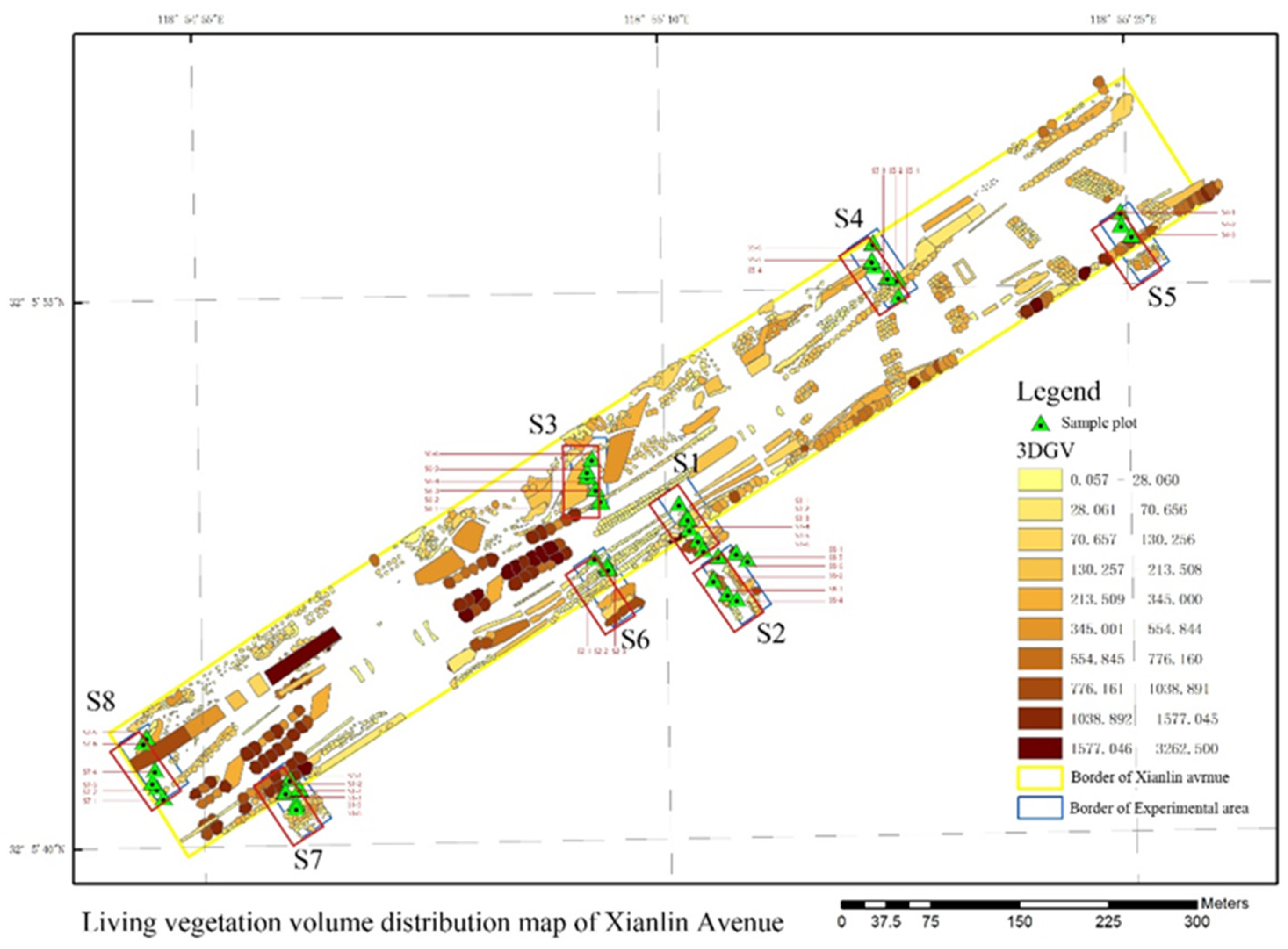
- The living vegetation volumes of the eight sample areas varied from 2038.73 m3 to 15,032.55 m3.
- Affected by different plant configurations, the living vegetation volumes in the sample areas showed obvious differences with an order of S7 > S2 > S3 > S1 > S5 > S6 > S8 > S4.
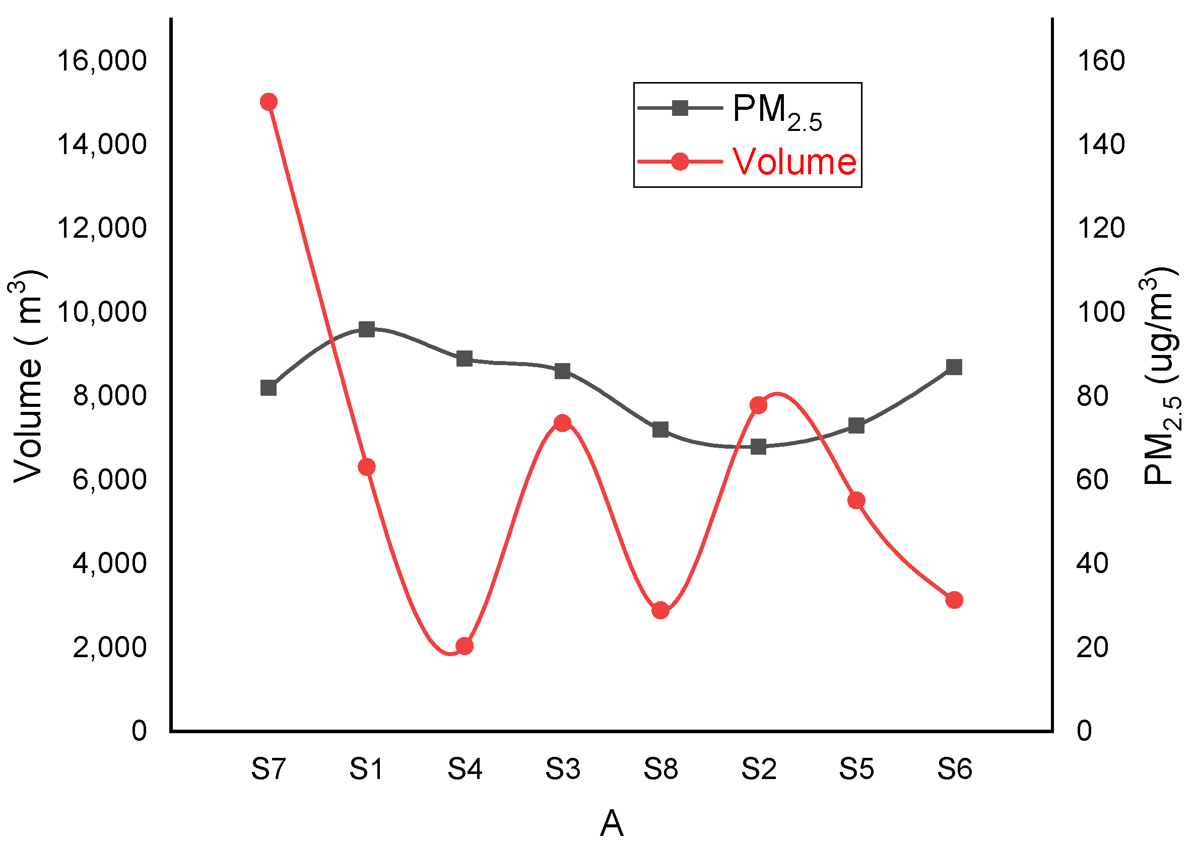
- The fitting relationship between living vegetation volumes and PM2.5 concentrations in different road green space is different owing to different compositions of plantings.
Abstract
1. Introduction
2. Study Sample and Method
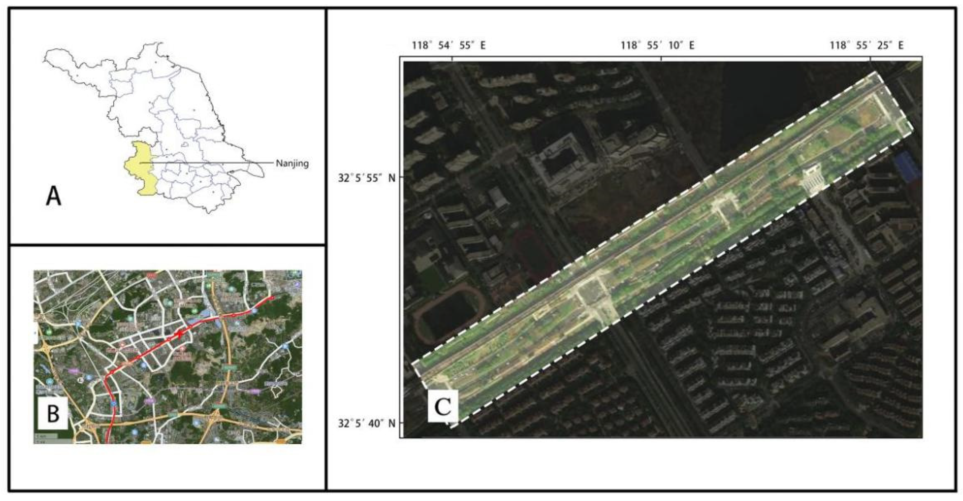
2.1. General Description of the Sampling Area
2.2. Distribution of Study Sample Areas and Monitoring Sites
2.3. Data Collection
- (1)
- PM2.5 concentration data collection
- (2)
- vegetation volume data collection
2.4. Analysis of PM2.5 Concentration Data
2.5. Calculation of Living Vegetation Volume
3. Results
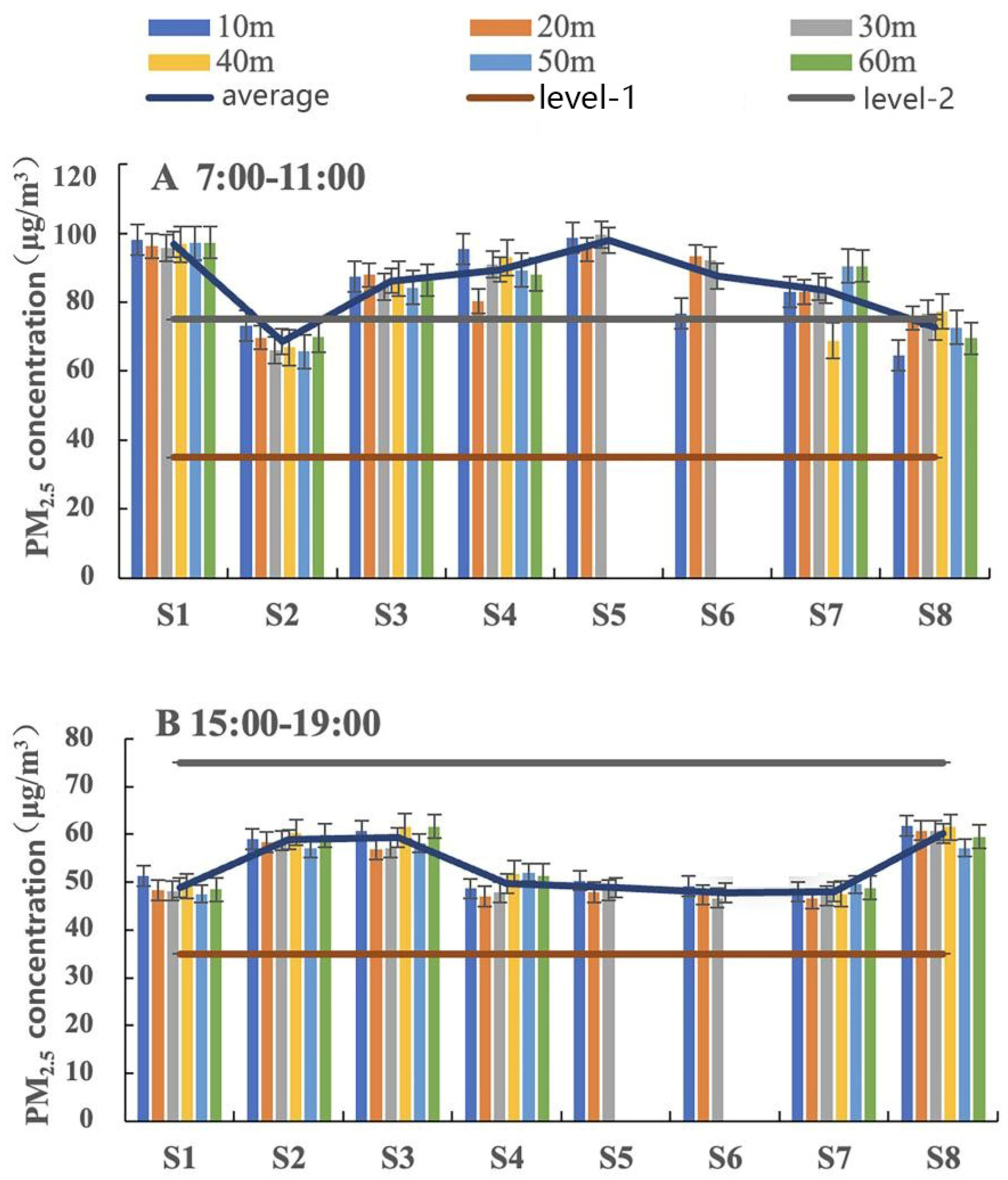
3.1. Variation of PM2.5 Concentrations at Monitoring Points in Different Sample Areas
3.2. Variation of PM2.5 Concentrations at Different Monitoring Points at the Same Distance from the Roadbed
3.3. Living Vegetation Volume Distribution in Different Sample Areas of Xianlin Avenue
3.4. Analysis of Living Vegetation Volumes and PM2.5 Concentrations
4. Discussion
4.1. Variability Analysis of PM2.5 Concentrations at Different Monitoring Points in the Eight Sample Areas
4.2. Fitting Analysis of Living Vegetation Volumes and PM2.5 Concentrations in the Sample Areas
5. Conclusions
Author Contributions
Funding
Institutional Review Board Statement
Informed Consent Statement
Data Availability Statement
Conflicts of Interest
Appendix A

| Type of Land Cover | ||||||
|---|---|---|---|---|---|---|
| Sample Area | Tree | Shrub | Herb | Road | River | Living Vegetation Volume Distribution in Sample Areas |
| S1 | Celtis sinensis, Salix babylonica, Populus simonii, Broussonetia papyrifera, Osmanthus fragrans | Ligustrum japonicum, Photinia × fraseri, Viburnum odoratissimum, Jasminum mesnyi | Cynodon dactylon | Bicycle lane, sidewalk | Yes | 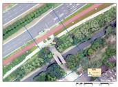 |
| S2 | Cinnamomum camphora, Ginkgo biloba, Osmanthus fragrans, Amygdalus persica, Myrica rubra | Loropetalum chinense var. rubrum, Nandina domestica, Euonymus japonicus var. aurea-marginatus, Prunus cerasifera f. atropurpurea, Rhododendron simsii, Ligustrum quihoui, Pittosporum tobira | Ophiopogon japonicus | Motorway, bicycle lane, sidewalk | No | 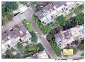 |
| S3 | Ligustrum lucidum, Cerasus serrulata, Platanus acerifolia, Osmanthus fragrans, Triadica sebifera, Ginkgo biloba | Ligustrum quihoui, Euonymus japonicus var. aurea-marginatus, Fatsia japonica, Arundo donax, Rosa chinensis, Pittosporum tobira | Cynodon dactylon | Bicycle lane, sidewalk | No | 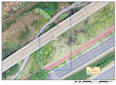 |
| S4 | Cinnamomum camphora, Cedrus deodara | Euonymus japonicus var. aurea-marginatus, Platycladus orientalis, Photinia × fraseri, Acer palmatum, Pittosporum tobira | Oxalis corymbosa, Coreopsis basalis, Pennisetum alopecuroides, Senecio cineraria, Miscanthus sacchariflorus | Bicycle lane, sidewalk | No | 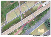 |
| S5 | Salix babylonic, Cerasus serrulata | Nerium oleander | Cynodon dactylon | Bicycle lane, sidewalk | Yes | 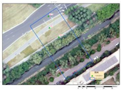 |
| S6 | Osmanthus fragrans, Broussonetia papyrifera | Nerium oleander | Oxalis corymbosa | Bicycle lane, sidewalk | Yes | 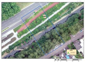 |
| S7 | Platanus acerifolia, Cedrus deodara, Pterocarya stenoptera, Metasequoia glyptostroboides | Photinia serratifolia, Boehmeria nivea | Cynodon dactylon | Bicycle lane, sidewalk | Yes |  |
| S8 | Cinnamomum camphora, Ginkgo biloba, Lagerstroemia. indica, Cerasus serrulata, Metasequoia glyptostroboides | Ligustrum × vicaryi, Photinia× fraseri, Euonymus japonicus var. aurea -marginatus, Fatsia japonica, Rhododendron simsii, Yucca gloriosa, Gardenia jasminoides, Hypericum monogynum, Pittosporum tobira | Cynodon dactylon | Bicycle lane, sidewalk | No | 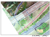 |
| NO. | Tree Species | Equation | Parameter | Correlation Coefficient | Crown Polygon Range (m) | |||
|---|---|---|---|---|---|---|---|---|
| a | b | c | R | R2 | ||||
| 1 | Salix babylonica | 0.832 | 0.042 | 0.758 | 0.758 | 0.575 ** | 1.95–10.67 | |
| 2 | Platanus acerifolia | −9.507 | 0.805 | - | - | 0.647 ** | 4.62–20.18 | |
| 3 | Pterocarya stenoptera | −4.23 | 0.592 | - | - | 0.350 ** | 3.0–19.35 | |
| 4 | Osmanthus fragrans | 11.296 | 0.004 | 0.918 | 0.918 | 0.843 ** | 1.25–10 | |
| 5 | Sophora japonica Linn. | 0.654 | 0.311 | 0.634 | 0.634 | 0.402 ** | 3.96–9.93 | |
| 6 | Magnolia grandiflora L. | −5.383 | 0.858 | - | - | 0.737 ** | 2.8–8.45 | |
| 7 | Acer palmatum | 1.927 | 0.604 | 0.926 | 0.926 | 0.858 ** | 0.8–7.25 | |
| 8 | Nerium oleander | 0.632 | 0.116 | 0.831 | 0.831 | 0.691 ** | 1.1–4.45 | |
| 9 | Ligustrum japonicum | 0.846 | 0.95 | - | - | 0.902 ** | 1.3–8.57 | |
| 10 | Cinnamomum camphora | 0.837 | 0.381 | 0.883 | 0.883 | 0.779 ** | 1.9–15.29 | |
| 11 | Cedrus deodara | −7.922 | 0.873 | - | - | 0.762 ** | 3.4–9.6 | |
| 12 | Ginkgo biloba | 0.304 | 0.603 | 0.891 | 0.891 | 0.793 ** | 1.3–22.68 | |
| 13 | Cerasus serrulata | 0 | 0 | - | - | 0 | 1.35–7.99 | |
| 14 | Lagerstroemia. indica | 1.172 | 0.305 | 0.381 | 0.381 | 0.145 ** | 1.1–2.5 | |
| 15 | Prunus cerasifera f. atropurpurea | −1.421 | 0.733 | - | - | 0.538 ** | 1.63–6.1 | |
| 16 | Triadica sebifera | 0.426 | 0.285 | 0.752 | 0.752 | 0.566 ** | 2.65–11.8 | |
| NO. | Shape of Canopy | Formula of Canopy Volume | Species |
|---|---|---|---|
| 1 | Ovoid | Broussonetia papyrifera, Ulmus pumilaL., Acer monoMaxim., Malus halliana Koehne | |
| 2 | Conic | Sabina chinensis (L.) Ant., Metasequoia glyptostroboides, Ilex latifolia Thunb. | |
| 3 | Spherical | Celtis sinensis Pers, PhotiniaserrulataLindl., Prunus persica ‘Duplex’, Eriobotrya japonica (Thunb.) Lindl | |
| 4 | Hemispherical | Ailanthus altissima (Mill.) Swingle | |
| 5 | Spheric fan-shaped | Melia azedarach L., Albizia julibrissin Durazz., Armeniaca mume Sieb. | |
| 6 | Bulbous imperfection | —— | |
| 7 | Cylindrical | —— |
| ANOVA | ||||||
|---|---|---|---|---|---|---|
| Sum of Squares | Variance | Mean Square | F | Data Significance | ||
| S7 | Between groups | 15,553.871 | 33 | 471.329 | 1.711 | 0.217 |
| Within group | 2203.600 | 8 | 275.450 | |||
| total | 17,757.471 | 41 | ||||
| S1 | Between groups | 19,877.905 | 33 | 602.361 | 3.273 | 0.041 |
| Within group | 1472.500 | 8 | 184.063 | |||
| total | 21,350.405 | 41 | ||||
| S3 | Between groups | 48,437.494 | 33 | 1467.803 | 13.894 | 0.000 |
| Within group | 845.125 | 8 | 105.641 | |||
| total | 49,282.619 | 41 | ||||
| S4 | Between groups | 49,636.476 | 33 | 1504.136 | 1.990 | 0.154 |
| Within group | 6046.000 | 8 | 755.750 | |||
| total | 55,682.476 | 41 | ||||
| S8 | Between groups | 57,022.601 | 33 | 1727.958 | 11.607 | 0.001 |
| Within group | 1191.000 | 8 | 148.875 | |||
| total | 58,213.601 | 41 | ||||
| S5 | Between groups | 53,684.294 | 33 | 1626.797 | 2.493 | 0.088 |
| Within group | 5219.569 | 8 | 652.446 | |||
| total | 58,903.863 | 41 | ||||
| S6 | Between groups | 22,810.476 | 33 | 691.227 | 2.589 | 0.080 |
| Within group | 2136.000 | 8 | 267.000 | |||
| total | 24,946.476 | 41 | ||||
| Single Sample Statistics | ||||
|---|---|---|---|---|
| Number of Cases | Average Value | Standard Deviation | Mean Value of Standard Error | |
| S7 | 42 | 82.9857 | 20.81127 | 3.21125 |
| S1 | 42 | 96.8810 | 22.81976 | 3.52117 |
| S4 | 42 | 89.4762 | 36.85253 | 5.68647 |
| S8 | 42 | 72.7262 | 37.68082 | 5.81428 |
| S2 | 42 | 68.5952 | 40.83701 | 6.30129 |
| S6 | 42 | 87.4762 | 24.66679 | 3.80617 |
| S3 | 42 | 86.2619 | 34.67009 | 5.34971 |
| S5 | 42 | 73.3690 | 37.90356 | 5.84865 |
| Single Sample Test | ||||||
|---|---|---|---|---|---|---|
| Inspection Value = 0 | ||||||
| t | Variance | Sig. (Double) | Mean Value Difference | 95% Confidence Interval of Difference | ||
| Lower Limit | Upper Limit | |||||
| S7 | 25.842 | 41 | 0.000 | 82.98571 | 76.5005 | 89.4710 |
| S1 | 27.514 | 41 | 0.000 | 96.88095 | 89.7698 | 103.9921 |
| S4 | 15.735 | 41 | 0.000 | 89.47619 | 77.9921 | 100.9602 |
| S8 | 12.508 | 41 | 0.000 | 72.72619 | 60.9840 | 84.4684 |
| S2 | 10.886 | 41 | 0.000 | 68.59524 | 55.8695 | 81.3209 |
| S6 | 22.983 | 41 | 0.000 | 87.47619 | 79.7895 | 95.1629 |
| S3 | 16.125 | 41 | 0.000 | 86.26190 | 75.4579 | 97.0659 |
| S5 | 12.545 | 41 | 0.000 | 73.36905 | 61.5575 | 85.1806 |
References
- Zhang, X.Y.; Sun, J.Y.; Wang, Y.Q.; Li, W.J.; Zhang, Q.; Wang, W.G.; Quan, J.N.; Cao, G.L.; Wang, J.Z.; Yang, Y.Q.; et al. Factors contributing to haze and fog in China. Chin. Sci. Bull. 2013, 58, 1178–1187. [Google Scholar] [CrossRef]
- Jia, C.; Tong, S.; Zhang, X. Atmospheric oxidizing capacity in autumn Beijing: Analysis of the O3 and PM2.5 episodes based on observation-based model. J. Environ. Sci. 2023, 124, 557–569. [Google Scholar] [CrossRef] [PubMed]
- Wang, Y.N.; Jia, C.H.; Tao, J.; Zhang, L.; Liang, X.; Ma, J.; Gao, H.; Huang, T.; Zhang, K. Chemical characterization and source apportionment of PM2.5 in a semi-arid and petrochemical-industrialized city Northwest China. Sci. Total Environ. 2016, 573, 1031–1040. [Google Scholar] [CrossRef] [PubMed]
- Xu, X.M.; Zhang, H.F.; Chen, J.M.; Li, Q.; Wang, X.; Wang, W.; Zhang, Q.; Xue, L.; Ding, A.; Mellouki, A. Six sources mainly contributing to the haze episodes and health risk assessment of PM2.5 at Beijing suburb in winter 2016. Ecotoxicol. Environ. Saf. 2018, 166, 146–156. [Google Scholar] [CrossRef]
- Wang, S. Effects of COVID-19 Control Measures on the Concentration and Composition of PM2.5-Bound Polycyclic Aromatic Hydrocarbons in Shanghai. Atmosphere 2023, 14, 95. [Google Scholar]
- Li, Y.; Liao, Q.; Zhao, X.G.; Bai, Y.; Tao, Y. Influence of PM2.5 pollution on health burden and economic loss in China. Environ. Sci. 2020, 42, 1688–1695. [Google Scholar] [CrossRef]
- Nanjing Ecological Environment Bureau. 2016 Nanjing Environment Status Bulletin. Available online: http://hbj.nanjing.gov.cn/njshjbhj/201706/t20170605_1325805.html (accessed on 19 December 2020).
- Nanjing Ecological Environment Bureau. 2017 Nanjing Environment Status Bulletin. (2018-06-05). Available online: Refhttp://hbj.nanjing.gov.cn/njshjbhj/201806/t20180605_1325808.html (accessed on 19 December 2020).
- Nanjing Ecological Environment Bureau. 2018 Nanjing Environment Status Bulletin. (2019-06-05). Available online: http://hbj.nanjing.gov.cn/njshjbhj/201906/t20190605_1559172.html (accessed on 19 December 2020).
- Nanjing Ecological Environment Bureau. 2019 Nanjing Environment Status Bulletin. (2020-06-03). Available online: http://hbj.nanjing.gov.cn/njshjbhj/202006/t20200603_1903785.html (accessed on 19 December 2020).
- Neofytou, P.; Venetsanos, A.G.; Rafailidis, S.; Bartzis, J.G. Numerical investigation of the pollution dispersion in an urban street canyon. Environ. Model. Softw. 2004, 21, 525–531. [Google Scholar] [CrossRef]
- Maji, K.J.; Ye, W.F.; Arora, M.; Nagendra, S.S. PM2.5-related health and economic loss assessment for 338 Chinese cities. Environ. Int. 2018, 121, 392–403. [Google Scholar] [CrossRef]
- Liu, C.Z.; Dai, A.Q.; Ji, Y.; Sheng, Q.Q.; Zhu, Z.L. Effect of Different Plant Communities on Fine Particle Removal in an Urban Road Greenbelt and Its Key Factors in Nanjing, China. Sustainability 2023, 15, 156. [Google Scholar] [CrossRef]
- Su, T.H.; Lin, C.S.; Lu, S.Y.; Lin, J.C.; Wang, H.H.; Liu, C.P. Effect of air quality improvement by urban parks on mitigating PM2.5 and its associated heavy metals: A mobile-monitoring field study. J. Environ. Manag. 2022, 323, 116283. [Google Scholar] [CrossRef]
- Beckett, K.P.; Freer-Smith, P.H.; Taylor, G. Effective tree species for local air quality management. J. Arboric. 2000, 26, 12–19. [Google Scholar]
- Freer-Smith, P.H.; El-Khatib, A.; Taylor, G. Capture of particulate pollution by trees: A comparison of species typical of semi-arid Areas (Ficus nitida and Eucalyptus globulus) with European and North American species. Water Air Soil Pollut. 2004, 155, 173–187. [Google Scholar] [CrossRef]
- Nowak, D.J.; Hirabayashi, S.; Bodine, A.; Hoehn, R. Modeled PM2.5 Removal by trees in ten US cities and associated health effects. Environ. Pollut. 2013, 178, 395–402. [Google Scholar] [CrossRef]
- Cavanagh, J.A.E.; Zawar-Reza, P.; Wilson, J.G. Spatial attenuation of ambient particulate matter air pollution within an urbanised native forest patch. Urban For. Urban Green. 2009, 8, 21–30. [Google Scholar] [CrossRef]
- Shu, M.; Si, R.M.J.; Jiang, T.; Zhao, X.L.; Yang, M.; Jin, C.Y.; Li, K.X.; Sun, M.Y. Retention capacity of the main urban afforest plant species for atmospheric particles in northwest of Liaoning province. J. Soil Water Conserv. 2018, 32, 297–303+309. [Google Scholar] [CrossRef]
- Li, X.X.; Tang, L.Y.; Peng, W.; Chen, J.X.; Ma, X. Estimation method of urban green space living vegetation volume based on backpack light detection and ranging. J. Appl. Ecol. 2022, 33, 2777–2784. [Google Scholar] [CrossRef]
- Chen, M.; Dai, F. Vegetation quantity in urban neighborhoods and its regulating effect on PM2.5: The case of Wuhan City. Chinese Society of Landscape Architecture. In Proceedings of the 2018 Annual Conference of the Chinese Society of Landscape Architecture, Guiyang, China, 20–22 October 2018. [Google Scholar]
- Miao, C.; Yu, S.; Zhang, Y.; Hu, Y.; He, X.; Chen, W. Assessing outdoor air quality vertically in an urban street canyon and its response to microclimatic factors. J. Environ. Sci. 2023, 124, 923–932. [Google Scholar] [CrossRef]
- Sheng, Q.Q. Practical evaluation of the capability of garden plants to reduce atmospheric NO2 and experimental study on the tolerance mechanism. Nanjing For. Univ. 2018, 46, 127–134. [Google Scholar]
- Leonard, R.J.; McArthur, C.; Hochuli, D.F. Particulate matter deposition on roadside plants and the importance of leaf trait combinations. Urban For. Urban Green. 2016, 20, 249–253. [Google Scholar] [CrossRef]
- Song, C.; He, J.; Wu, L.; Jin, T.; Chen, X.; Li, R.; Ren, P.; Zhang, L.; Mao, H. Health burden attributable to ambient PM2.5 in China. Environ. Pollut. 2017, 223, 575–586. [Google Scholar] [CrossRef]
- Luo, G.; Wang, T.J.; Zhao, M.; Wang, D.Y.; Cao, Y.Q.; Chen, C. Chemical composition and source apportionment of fine particulate matter in Xianlin area of Nanjing based on on-line measurement. China Environ. Sci. 2020, 40, 1857–1868. [Google Scholar] [CrossRef]
- Guo, H.W.; Ding, G.D.; Zhao, Y.Y.; Gao, G.L.; Chen, M.X.; Wang, H.Y.; Lai, W.H. Diurnal variations in the mass concentration of suspended particulate matter (PM2.5) of different urban green space. Sci. Soil Water Conserv. 2013, 11, 99–103. [Google Scholar] [CrossRef]
- Zhou, J.; Sun, T. Study on remote sensing model of three dimensional green biomass and the estimation of environmental benefits of greenery. Remote Sens. Environ. 1995, 10, 162–174. [Google Scholar]
- Zhou, J. Study on the indexes of urban plant community. J. Chin. Landsc. Archit. 1998, 14, 61–63. [Google Scholar]
- Zhou, Y.; Zhou, J. The urban eco-environ-mental estimating system based on 3-dimension vegetation quantity. J. Chin. Landsc. Archit. 2001, 5, 78–80. [Google Scholar]
- Liang, H.; Li, W.; Zhang, Q.; Zhu, W.; Chen, D.; Liu, J.; Shu, T. Using unmanned aerial vehicle data to assess the three-dimension green quantity of urban green space: Acase study in Shanghai, China. Landsc. Urban Plan. 2017, 164, 81–90. [Google Scholar] [CrossRef]
- Sheng, Q.; Zhang, Y.; Zhu, Z.; Li, W.; Xu, J.; Tang, R. An experimental study to quantify road greenbelts and their association with PM2.5 concentration along city main roads in Nanjing, China. Sci. Total Environ. 2019, 667, 710–717. [Google Scholar] [CrossRef]
- Zhang, L.Y.; Qin, H. Analysis of dust-retention effect on PM2.5 and its variation in green belts of urban roads. Chin. Lands. Archit. 2015, 31, 106–110. [Google Scholar] [CrossRef]
- Kim, S.; Lee, S.; Hwang, K.; An, K. Exploring sustainable street tree planting patterns to be resistant against fine particles (PM2.5). Sustainability 2017, 9, 1709. [Google Scholar] [CrossRef] [Green Version]
- Viljami, V.; Thomas, H.W.; Zhao, W.L.; Yli-Pelkonen, V.; Mikola, J.; Pouyat, R.; Setälä, H. The effects of trees on air pollutant levels in peri-urban near-road environments. Urban For. Urban Green. 2018, 30, 62–71. [Google Scholar] [CrossRef]
- Jeanjean, A.P.R.; Monks, P.S.; Leigh, R.J. Modelling the effectiveness of urbantrees and grass on PM2.5 reduction via dispersion and deposition at a cityscale. Atmos. Environ. 2016, 147, 1–10. [Google Scholar] [CrossRef] [Green Version]
- Wang, J.J.; Xia, X.S.; Cheng, X.F. Temporal and spatial distribution characteristics and influencing factors of PM2.5 concentrations in Hefei City. Resour. Environ. Yangtze Basin 2020, 29, 1413–1421. [Google Scholar] [CrossRef]
- Zhang, B.B.; Wu, W.Z.; Sun, F.B.; Qi, F.; Yan, H.; Shao, F. A study of mutative factors to PM2.5 in green spaces with different arrangements of plants in winter. J. Chin. Urban For. 2019, 17, 25–30. [Google Scholar]
- Li, X.Y.; Zhao, S.T.; Li, Y.M.; Guo, J. The evaluation of particulate matter retention capability of common ornamental plants in the north of China. Chin. Landsc. Archit. 2015, 3, 72–75. [Google Scholar] [CrossRef]
- Wang, F.; Xiong, S.G.; Li, H.Y.; Li, L.L.; Zhang, Q.M.; He, M.X. Study on dust-retention capacity of major afforestation tree species in Tianjin Airport Economic Zone. J. Arid. Land Resour. Environ. 2015, 29, 100–104. [Google Scholar] [CrossRef]
- Sun, X.D.; Li, H.M.; Guo, X. Atmospheric particulate retention capacity of ten shrub species. Chin. Environ. Eng. 2017, 11, 1047–1054. [Google Scholar] [CrossRef]
- Lu, W.; Wang, H.L.; Zhu, B.; Shi, S.S.; Kang, H. Distribution characteristics of PM2.5 mass concentration and their impacting factors including meteorology and transmission in North Suburb of Nanjing during 2014 to 2016. Acta Sci. Circumst. 2019, 39, 1039–1048. [Google Scholar] [CrossRef]
- Liu, X.H.; Yu, X.X.; Zhang, Z.M. PM2.5 concentration differences between various forest types and its correlation with forest structure. Atmosphere 2015, 6, 1801–1815. [Google Scholar] [CrossRef] [Green Version]


| Pollutant Name | Average Time | Limit of Concentration | Unit | |
|---|---|---|---|---|
| Level 1 | Level 2 | |||
| PM2.5 | Average annual | 15 | 35 | μg/m3 |
| 24 h average | 35 | 75 | ||
Disclaimer/Publisher’s Note: The statements, opinions and data contained in all publications are solely those of the individual author(s) and contributor(s) and not of MDPI and/or the editor(s). MDPI and/or the editor(s) disclaim responsibility for any injury to people or property resulting from any ideas, methods, instructions or products referred to in the content. |
© 2023 by the authors. Licensee MDPI, Basel, Switzerland. This article is an open access article distributed under the terms and conditions of the Creative Commons Attribution (CC BY) license (https://creativecommons.org/licenses/by/4.0/).
Share and Cite
Liu, C.; Dai, A.; Zhang, H.; Sheng, Q.; Zhu, Z. Study on the Correlation Mechanism between the Living Vegetation Volume of Urban Road Plantings and PM2.5 Concentrations. Sustainability 2023, 15, 4653. https://doi.org/10.3390/su15054653
Liu C, Dai A, Zhang H, Sheng Q, Zhu Z. Study on the Correlation Mechanism between the Living Vegetation Volume of Urban Road Plantings and PM2.5 Concentrations. Sustainability. 2023; 15(5):4653. https://doi.org/10.3390/su15054653
Chicago/Turabian StyleLiu, Congzhe, Anqi Dai, Huihui Zhang, Qianqian Sheng, and Zunling Zhu. 2023. "Study on the Correlation Mechanism between the Living Vegetation Volume of Urban Road Plantings and PM2.5 Concentrations" Sustainability 15, no. 5: 4653. https://doi.org/10.3390/su15054653