
Integrating GIS, Statistical, Hydrogeochemical Modeling and Graphical Approaches for Hydrogeochemical Evaluation of Ad-Dawadmi Ground Water, Saudi Arabia: Status and Implications of Evaporation and Rock–Water Interactions


Abstract
:
1. Introduction
- (a)
- Evaluate the hydrogeochemical status and understand the implications of evaporation, rock–water interactions, and the interplaying factors;
- (b)
- Identify the GW chemistry’s hydrogeochemical characteristics in the AdDawadimi governorate and its nearby environs, Riyadh region, Saudi Arabia.
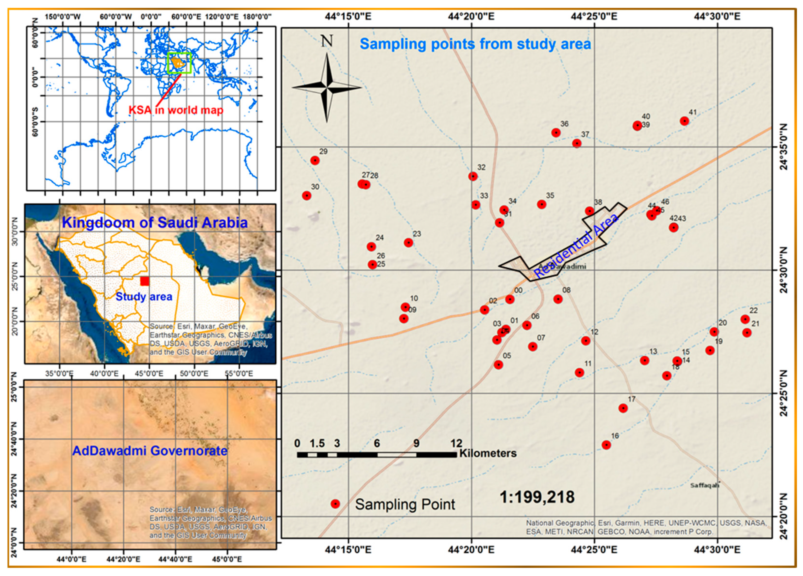
1.1. The Study Area
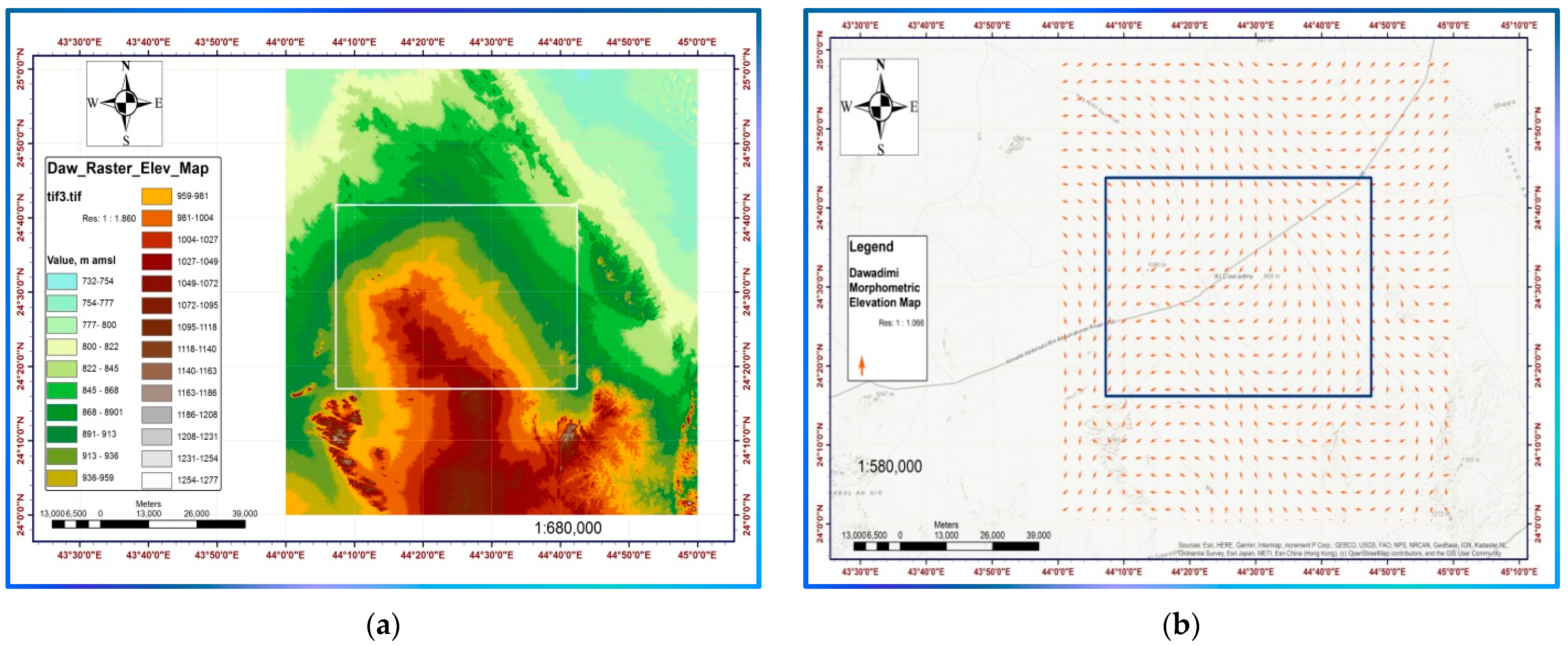
1.1.1. Location, Physiography, and Climate
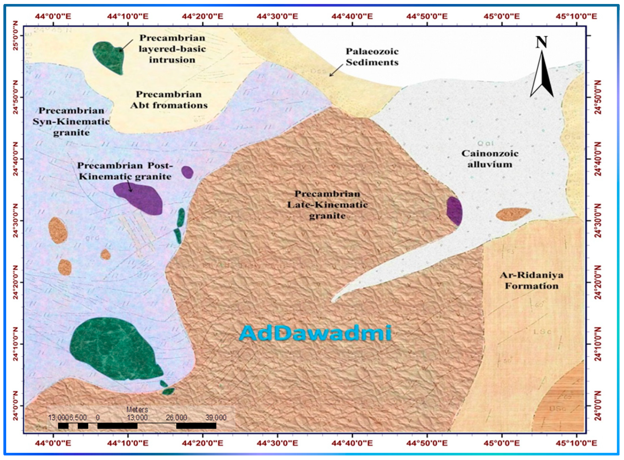
1.1.2. Geological Settings
2. Materials and Methods
2.1. Sampling and Preservation
2.2. Analyses and Procedures
2.3. Hydrochemical Characterization
2.4. Statistical Analyses
2.5. Geospatial and Geostatistical Analyses
2.6. Analysis of the Hydrogeochemical Water Quality
3. Results and Discussion
3.1. Water Quality Characterization
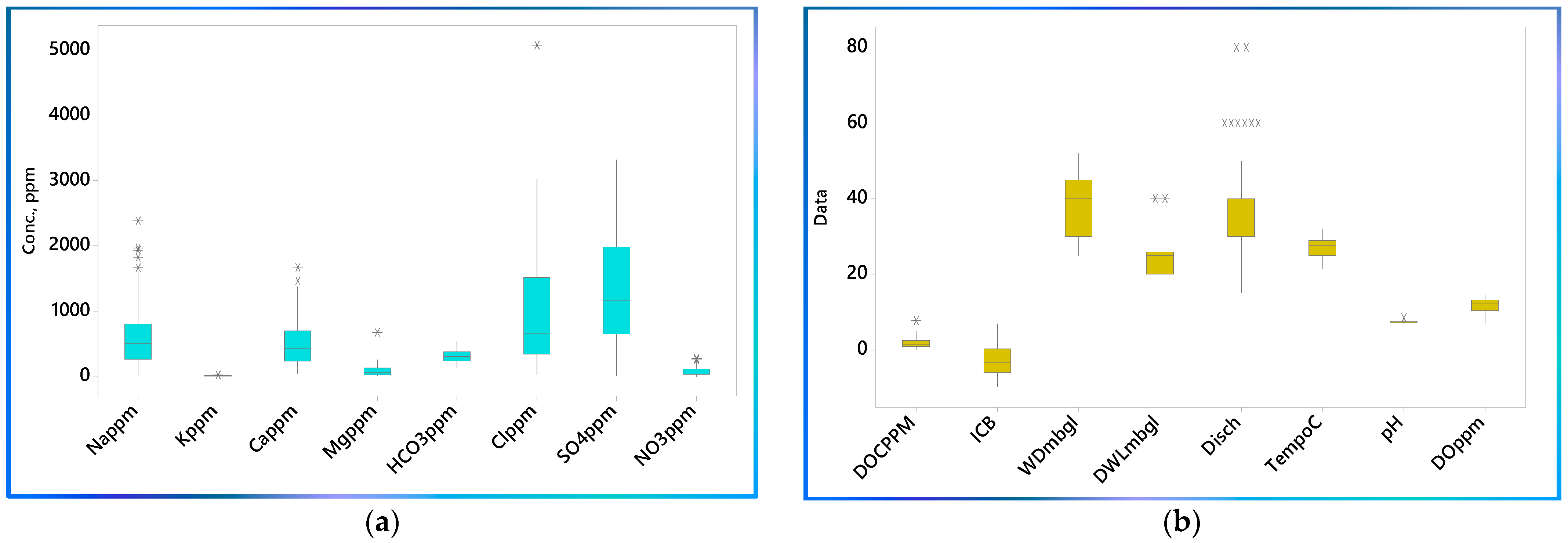
3.2. Major Constituents Analysis
3.3. Classification of Groundwater Using Geochemical Diagrams
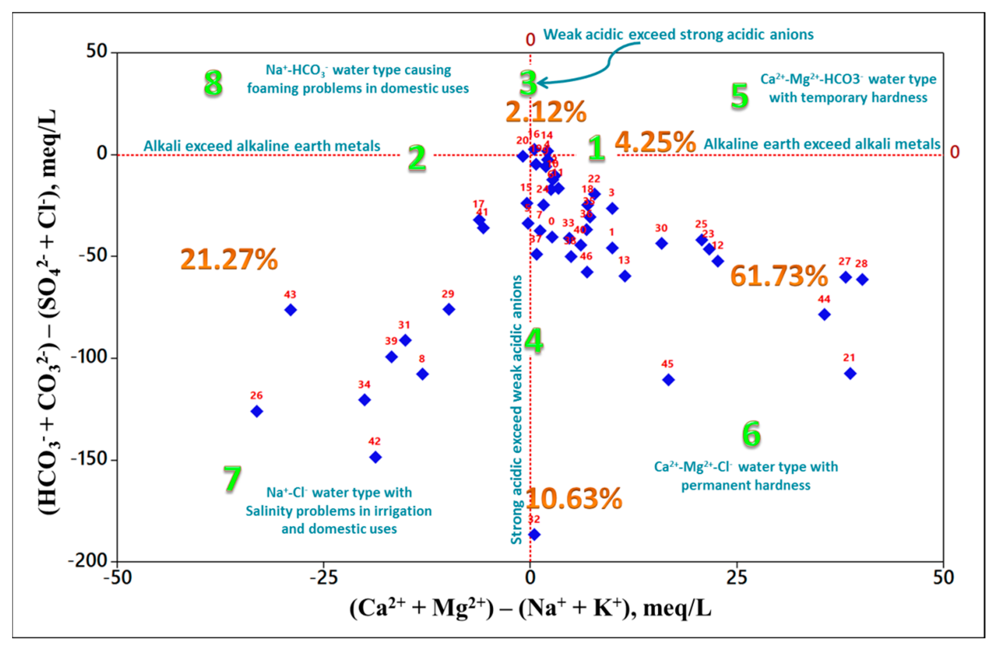
3.3.1. Chadha Plot
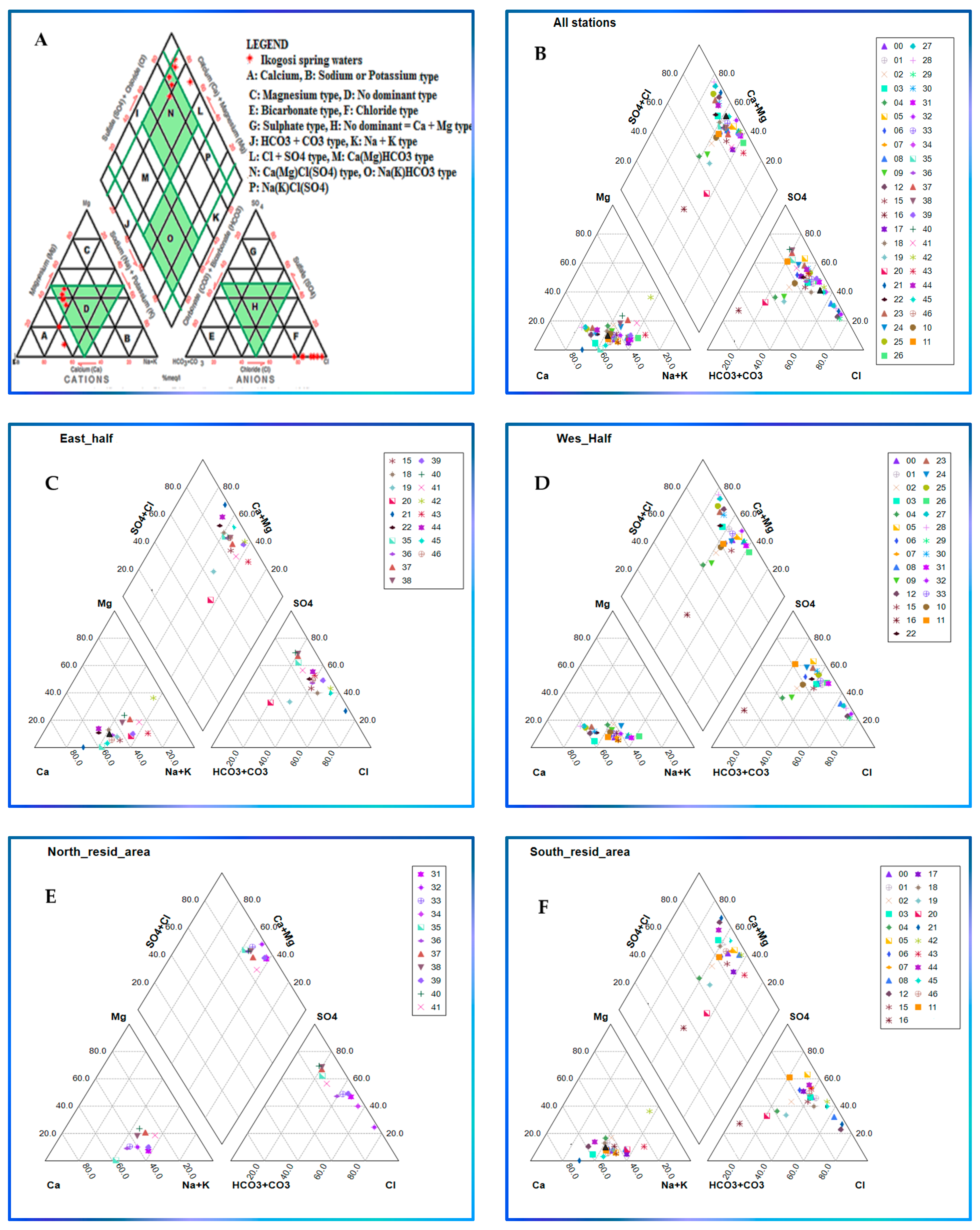
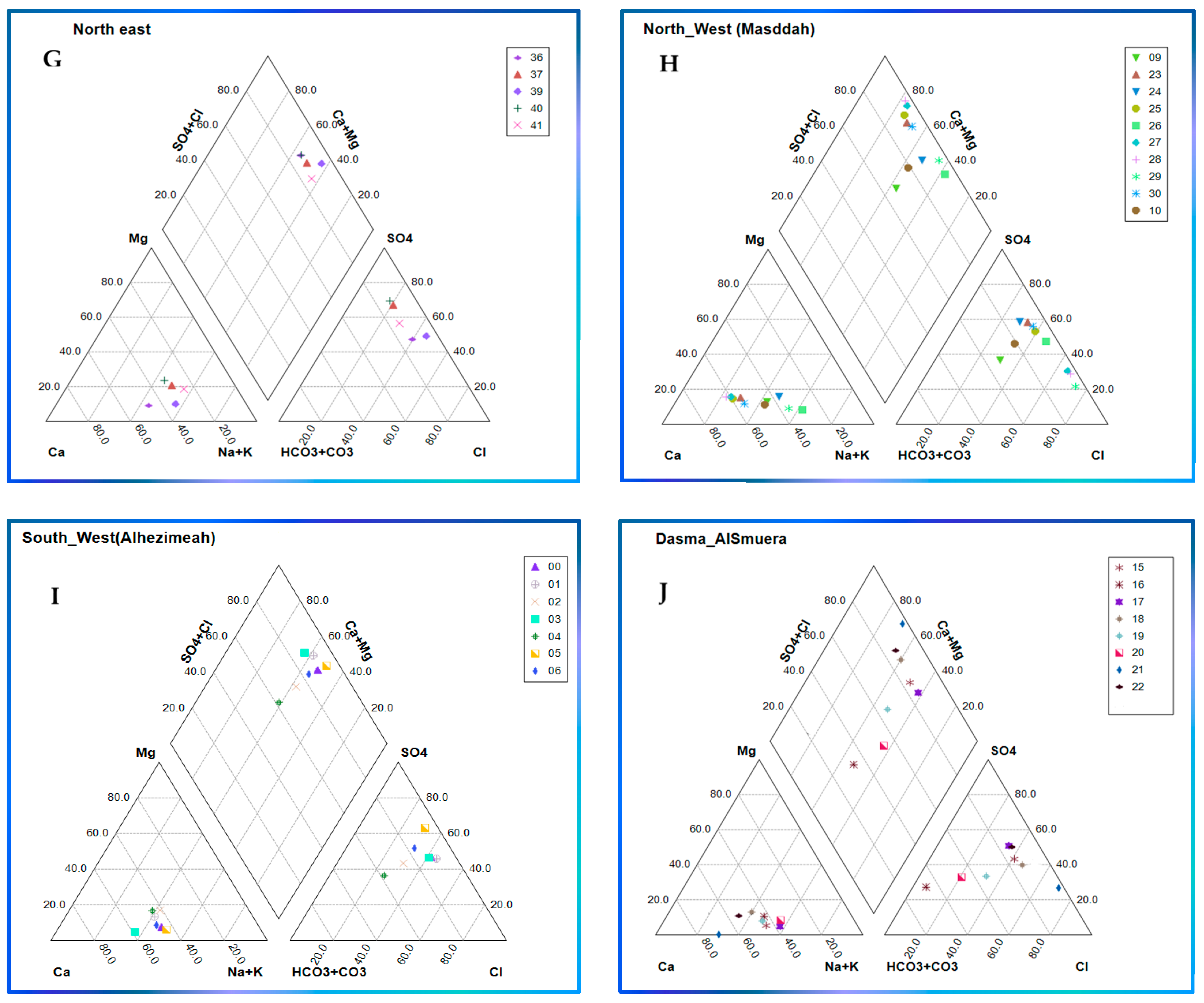
3.3.2. Piper Plot
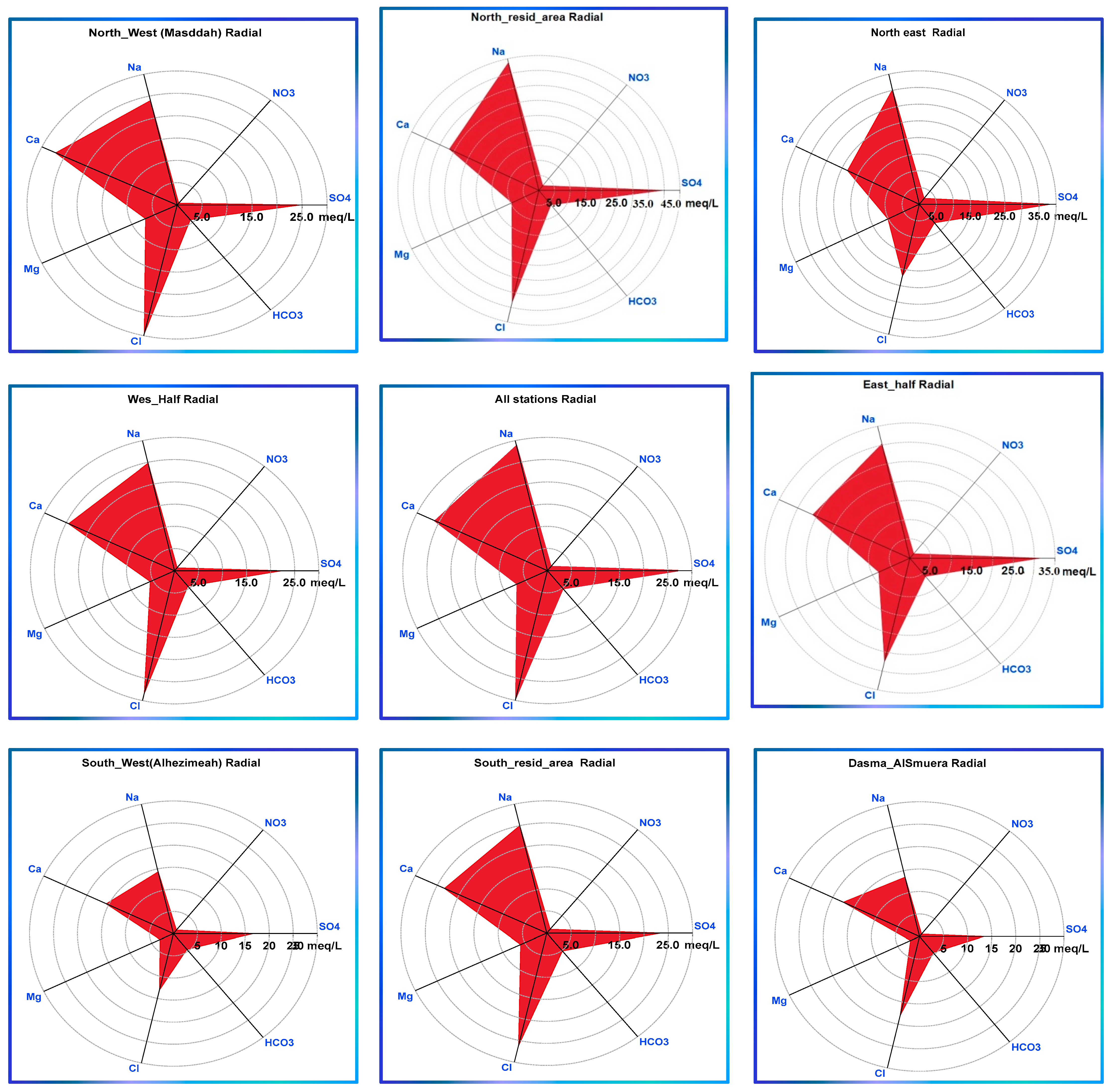
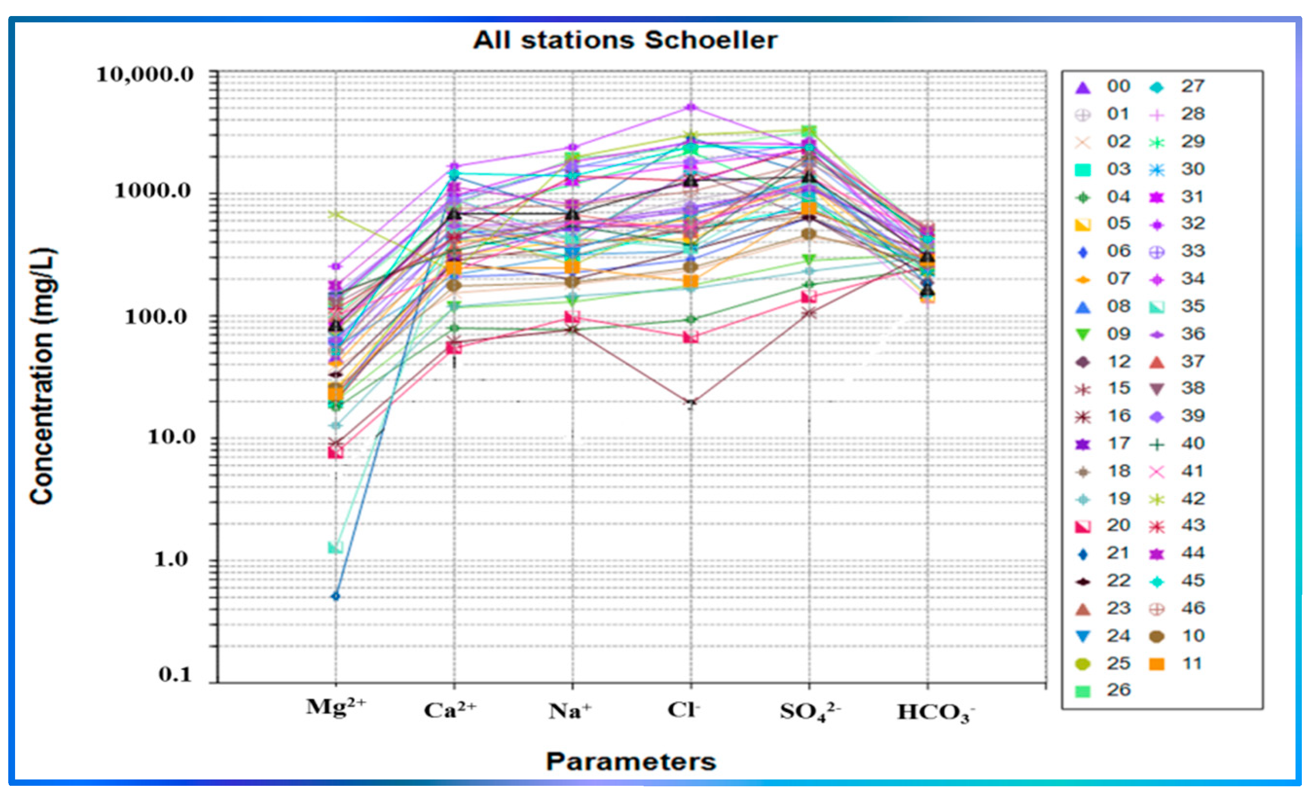
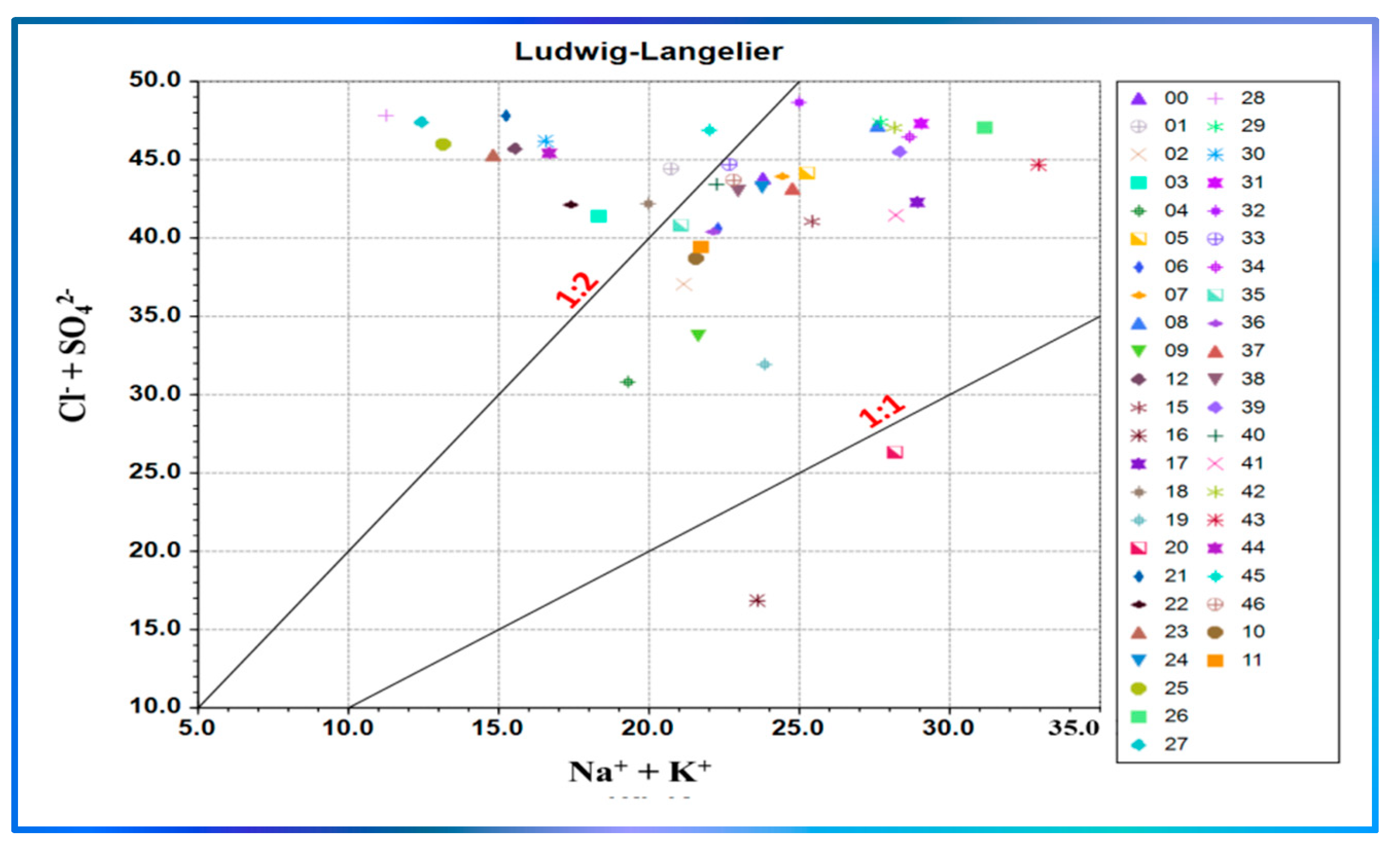
3.3.3. Schoeller Diagram and Ludwig–Langelier Plot
3.4. Major Ionic Species
3.5. Processes Controlling GW Hydrogeochemistry
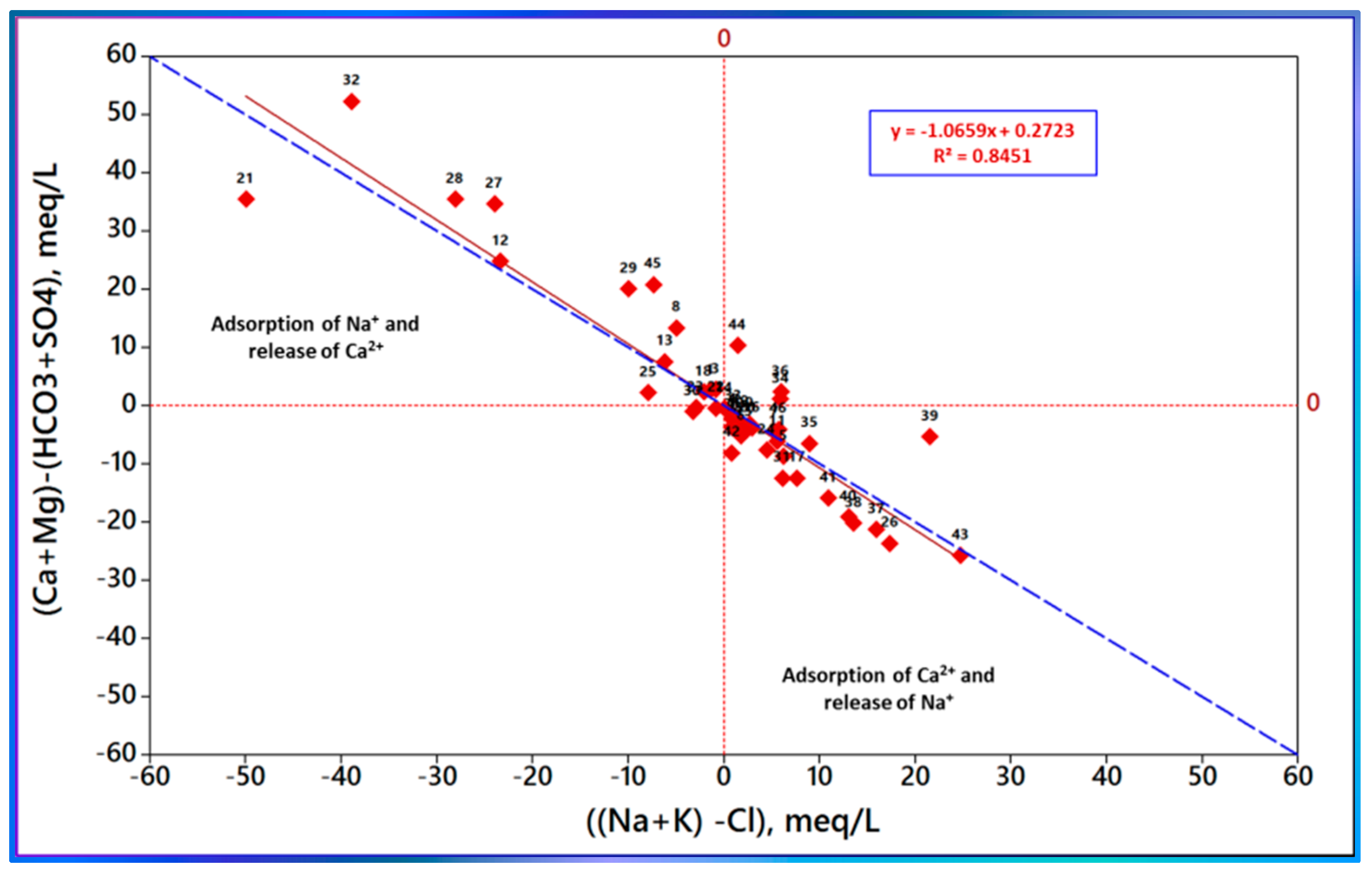
3.6. Ion Exchange Process
3.7. Hydrogeochemical Analysis Using Visual MINTEQ
3.8. Correlation Statistical Analysis
4. Conclusions
- a.
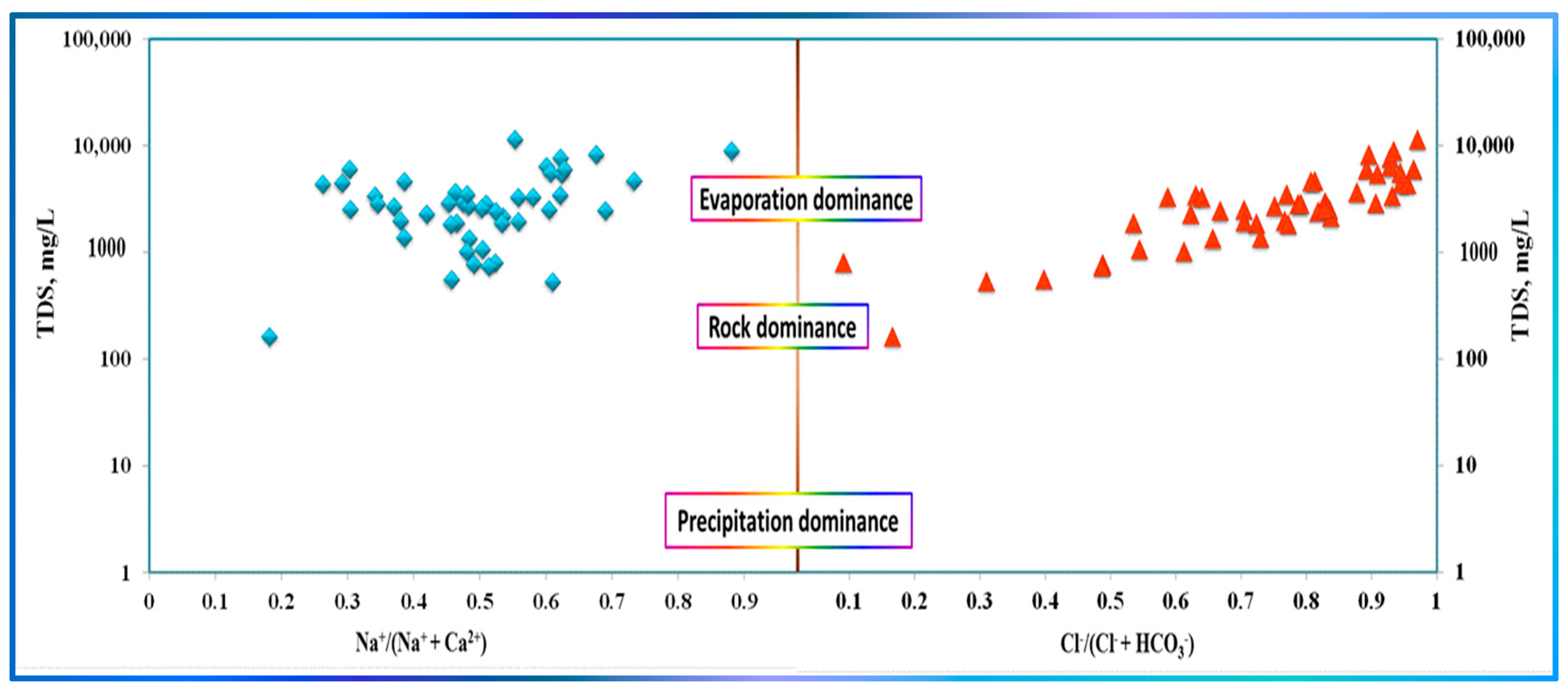
- Many co-occurring processes control the GW system’s evolution in the region: anthropogenic-driven evaporation, ion exchange (direct and reverse), precipitation of calcium salts, dissolution of soil salts, and rock weathering.
- b.
- The establishment of the vicious salinization cycle due to hyper-aridity, intensive agricultural activities, and higher daylight temperatures. This cycle poses immense deteriorating stresses on the quality of the GW reserve in the region.
- c.
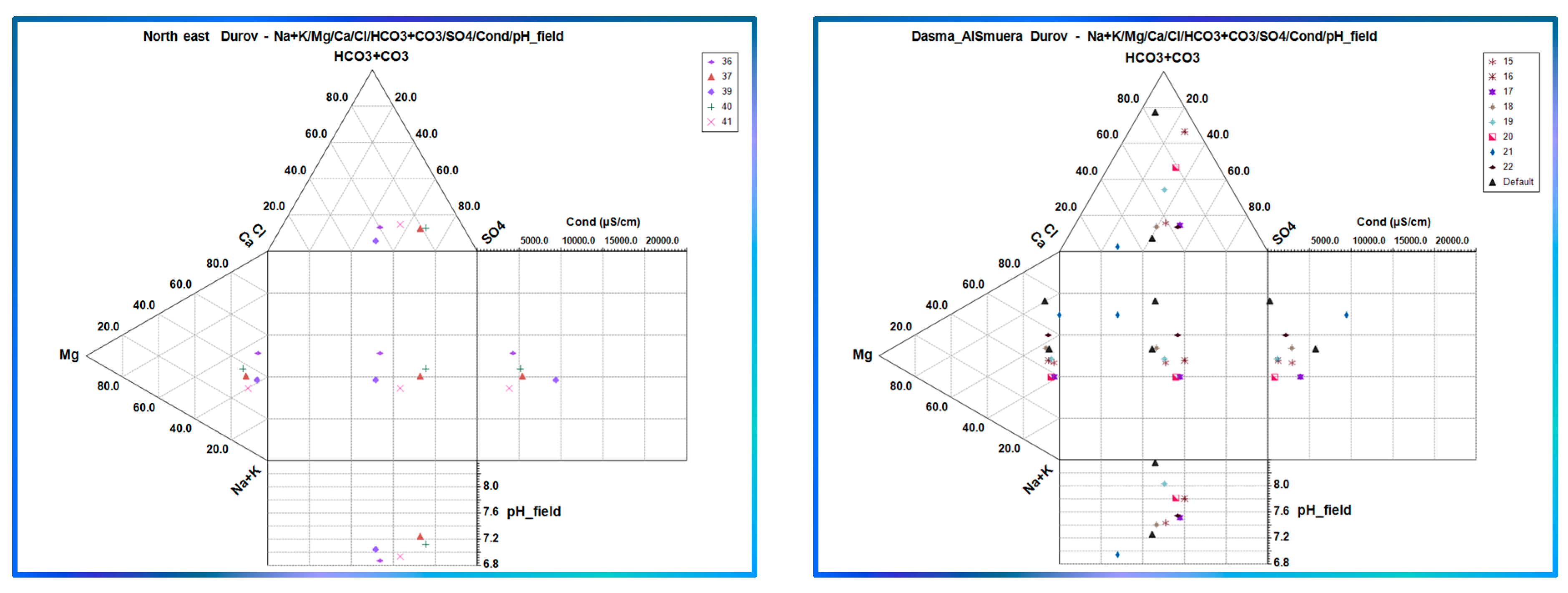
- Partitioning the study area into small portions on a spatial basis aided in mining useful information, allowing demarcating variations among localities in the case of relationships lacking spatial distribution ability such as Piper, radial, and Durov plots.
- d.
- The Hydrogeochemical modeling inferred the oversaturation of many minerals due to higher levels of EC and pH. The computed SIs are not normally distributed with as high skewness and Kurtosis values as those from the original data except for those of halite, which exhibit the lowest skewness and Kurtosis values, suggesting the existence of significant processes that impact the major individual constituents that may undergo input/output (solubilization/precipitation) effects.
- e.
- The largest regression and correlation coefficients are observed for the conservative and quasi-conservative ions, further supporting that evaporation significantly impacts the system.
- f.
- Localities exhibiting peaks of ECs, NO3−, SO42−, Cl−, Na+, and Ca2+ are identified, demarcating the effects of localized point source activities and evaporation-driven concentrating processes rather than those of lithology, catchment, or basin-wise ones.
- g.
- Integrating different approaches constrained the findings and interpretations, providing multiple lines of evidence that usefully supported or declined those that might be masked.
- h.
- Human activities, mainly agriculture, greatly impact the region’s GW system. Hence, remediation plans and protection policies to be in place are highly recommended to prevent overexploitation of the reserve and, simultaneously, remediate and brook the established vicious salinization cycle.
- i.
- Implementing and even enforcing recent irrigation systems’ adoption by the region’s peoples could help relieve the continuous ramping problem.
Author Contributions
Funding
Institutional Review Board Statement
Informed Consent Statement
Data Availability Statement
Conflicts of Interest
References
- Kajenthira, A.; Siddiqi, A.; Anadon, L.D. A new case for promoting wastewater reuse in Saudi Arabia: Bringing energy into the water equation. J. Environ. Manag. 2012, 102, 184–192. [Google Scholar] [CrossRef]
- Drewes, J.; Garduño, C.; Amy, G. Water reuse in the kingdom of Saudi Arabia—Status, prospects, and research needs. Water Sci. Technol. Water Supply 2012, 12, 926–936. [Google Scholar] [CrossRef]
- FAO. Irrigation in the Middle East Region in Figures: AQUASTAT Survey 2008; FAO Water Reports; FAO: Roma, Italy, 2008. [Google Scholar]
- Chowdhury, S.; Al-zahrani, M. Implications of Climate Change on Water Resources in Saudi Arabia. Arab. J. Sci. Eng. 2013, 38, 1959–1971. [Google Scholar] [CrossRef]
- Chowdhury, S.; Al-zahrani, M. Characterizing water resources and trends of sector-wise water consumptions in Saudi Arabia. J. King Saud Univ. Eng. Sci. 2013, 27, 68–82. [Google Scholar] [CrossRef] [Green Version]
- Chowdhury, S.; Al-zahrani, M. Water Resources And Water Consumption Pattern In Saudi Arabia. In Proceedings of the 10th Gulf Water Conference, Doha, Qatar, 22–24 April 2012; pp. 67–81. [Google Scholar]
- Haider, H.; Ghumman, A.; Al-salamah, I.; Thabit, H. Assessment Framework for Natural Groundwater Contamination in Arid Regions: Development of Indices and Wells Ranking System Using Fuzzy VIKOR Method. Water 2020, 12, 423. [Google Scholar] [CrossRef] [Green Version]
- Wang, J.; Yang, Y. An approach to catchment-scale groundwater nitrate risk assessment from diffuse agricultural sources: A case study in the Upper Bann, Northern Ireland. Hydrol Process. 2008, 4286, 4274–4286. [Google Scholar] [CrossRef]
- Al-Zaidi, A.; Elhag, E.; Al-Otaibi, S.; Baig, M. Negative effects of pesticides on the environment and the farmers awareness in Saudi Arabia: A case study. J. Anim. Plant Sci. 2011, 21, 605–611. [Google Scholar]
- Alhawas, A.A. Towards sustainable water resources for arid land cities: The case of Riyadh. WIT 2011, 145, 87–98. [Google Scholar] [CrossRef]
- Alrasheedi, N.H. An Analysis of Renewable Water Sources in Saudi Arabia. Am. J. Clim. Chang. 2014, 3, 413–419. [Google Scholar] [CrossRef] [Green Version]
- Benaafi, M.; Al-shaibani, A. Hydrochemical and Isotopic Investigation of the Groundwater from Wajid Aquifer in Wadi Al-Dawasir, Southern Saudi Arabia. Water 2021, 13, 1855. [Google Scholar] [CrossRef]
- Zaidi, F.; Mogren, S.; Mukhopadhyay, M.; Ibrahim, E. Evaluation of groundwater chemistry and its impact on drinking and irrigation water quality in the eastern part of the Central Arabian graben and trough system, Saudi Arabia. J. African Earth Sci. 2016, 120, 208–219. [Google Scholar] [CrossRef]
- Kumar, P.; Mahajan, A.; Kumar, A. Groundwater geochemical facie: Implications of rock-water interaction at the Chamba city (HP), northwest Himalaya, India. Environ. Sci. Pollut. Res. 2020, 27, 9012–9026. [Google Scholar] [CrossRef]
- Dehnavi, A.G.; Sarikhani, R.; Nagaraju, D. Hydro geochemical and rock water interaction studies in East of Kurdistan, NW of Iran. Int. J. Environ. Sci Res. 2011, 1, 16–22. [Google Scholar]
- Subramani, T.; Rajmohan, N.; Elango, L. Groundwater geochemistry and identification of hydrogeochemical processes in a hard rock region, Southern India. Environ. Monit. Assess. 2010, 162, 123–137. [Google Scholar] [CrossRef]
- Su, Y.-H.; Feng, Q.; Zhu, G.-F.; Si, J.-H.; Zhang, Y.-W. Identification, and Evolution of Groundwater Chemistry in the Ejin Sub-Basin of the Heihe River, Northwest China. Pedosphere 2007, 17, 331–342. [Google Scholar] [CrossRef]
- Ren, C.; Zhang, Q. Groundwater Chemical Characteristics and Controlling Factors in a Region of Northern China with Intensive Human Activity. Int. J. Environ. Res. Public Health 2020, 17, 9126. [Google Scholar] [CrossRef] [PubMed]
- Biglari, H.; Chavoshani, A.; Javan, N.; Mahvi, A.H. Geochemical study of groundwater conditions with special emphasis on fluoride concentration, Iran, Desalin. Water Treat. 2016, 57, 22392–22399. [Google Scholar] [CrossRef]
- Glynn, P.; Plummer, L. Geochemistry and the understanding of ground-water systems. Hydrogeol. J. 2005, 13, 263–287. [Google Scholar] [CrossRef]
- Herczeg, A.L.; Dogramaci, S.S.; Leaney, F.W.J. Origin of dissolved salts in a large, semi-arid groundwater system: Murray Basin, Australia. Mar. Freshw. Res. 2001, 52, 41–52. [Google Scholar] [CrossRef]
- Nachshon, U.; Weisbrod, N.; Dragila, M.; Grader, A. Combined evaporation and salt precipitation in homogeneous and heterogeneous porous media. Water Resour. Res. 2011, 47, 1–16. [Google Scholar] [CrossRef]
- Abbasnia, A.; Alimohammadi, M.; Mahvi, A.H.; Nabizadeh, R.; Yousefi, M.; Pasalari, H.; Mirzabeigi, M. Assessment of groundwater quality and evaluation of scaling and corrosiveness potential of drinking water samples in villages of Chabahr city, Sistan and Baluchistan province in Iran. Data Brief 2018, 16, 182–192. [Google Scholar] [CrossRef]
- Ijumulana, J.; Ligate, F.; Bhattacharya, P.; Mtalo, F.; Zhang, C. Spatial analysis and GIS mapping of regional hotspots and potential health risk of fluoride concentrations in groundwater of northern Tanzania. Sci. Total Environ. 2020, 735, 139584. [Google Scholar] [CrossRef]
- Fatima, S.; Khan, M.; Siddiqui, F.; Mahmood, N.; Salman, N.; Alamgir, A.; Shaukat, S. Geospatial assessment of water quality using principal components analysis (PCA) and water quality index (WQI) in Basho Valley, Gilgit Baltistan (Northern Areas of Pakistan). Environ. Monit. Assess. 2022, 194, 151. [Google Scholar] [CrossRef]
- Mohamed, A.; Asmoay, A.; Alshehri, F.; Abdelrady, A.; Othman, A. Hydro-Geochemical Applications and Multivariate Analysis to Assess the Water–Rock Interaction in Arid Environments. Appl. Sci. 2022, 12, 6340. [Google Scholar] [CrossRef]
- Ahmed, I.; Nazzal, Y.; Zaidi, F.K.; Al-Arifi, N.; Ghrefat, H.; Naeem, M. Hydrogeological vulnerability and pollution risk mapping of the Saq and overlying aquifers using the DRASTIC model and GIS techniques, NW Saudi Arabia. Environ. Earth Sci. 2015, 74, 1303–1318. [Google Scholar] [CrossRef]
- Ijumulana, J.; Ligate, F.; Irunde, R.; Bhattacharya, P.; Ahmad, A.; Tomašek, I.; Maity, J.P.; Mtalo, F. Spatial variability of the sources and distribution of fluoride in groundwater of the Sanya alluvial plain aquifers in northern Tanzania. Sci. Total. Environ. 2022, 810, 152153. [Google Scholar] [CrossRef] [PubMed]
- Abdelkader, M.; Al-amoud, A.; El, M.; El-feky, A. Remote Sensing Applications: Society and Environment Assessment of flash flood hazard based on morphometric aspects and rainfall-runoff modeling in Wadi Nisah, central Saudi Arabia. Remote Sens. Appl. Soc. Environ. 2021, 23, 100562. [Google Scholar]
- Gomaa, H.; Alotibi, A.; Charni, M.; Almarri, A.; Gomaa, F. Conceptual Evaluation of Factors Controlling Groundwater Chemistry in Ad-Dawadmi, Saudi Arabia, Using Visualization and Multiple Lines of Evidence, Water (Switzerland). Water 2022, 14, 1857. [Google Scholar] [CrossRef]
- Gomaa, H.; Charni, M.; Alotibi, A.A.; AlMarri, A.; Gomaa, F. Spatial Distribution, and Hydrogeochemical Factors Influencing the Occurrence of Total Coliform and E. coli Bacteria in Groundwater in a Hyperarid Area, Ad-Dawadmi, Saudi Arabia. Water 2022, 14, 3471. [Google Scholar] [CrossRef]
- Ahmed, M.; Aqnouy, M.; El Messari, J.S. Sustainability of Morocco’s groundwater resources in response to natural and anthropogenic forces. J. Hydrol. 2021, 603, 126866. [Google Scholar] [CrossRef]
- El-Didy, S. Evaluation of The Proposed Drainage Network for Lowering the Groundwater Levels in Al-Dawadmi Town. J. King Abdulaziz Univ. Environ. Arid L. Agric. Sci. 1997, 8, 111–123. [Google Scholar] [CrossRef]
- AdDawadmi_Gover. 2022. Available online: https://en.wikipedia.org/wiki/Dawadmi (accessed on 12 March 2022).
- Timeanddate, Climate and Weather Averages in Ad Dawadmi, Saudi Arabia, Timeanddate. 2022. Available online: https://www.timeanddate.com/weather/saudi-arabia/dawadmi/climate (accessed on 12 March 2022).
- Johnson, P.R. Explanatory Notes To the Map of Proterozoic Geology of Western Saudi Arabia; Saudi Geological Survey-Riyadh Office: Jeddah, Saudi Arabia, 2006. [Google Scholar]
- Al Shanti, M.S. The Geology and Mineralization of the Ad-Dawadmi District of Saudi Arabia. Ph.D. Thesis, Imperial College London, London, UK, 1973. [Google Scholar]
- El-Sawy, E.; Eldougdoug, A.; Gobashy, M. Geological and geophysical investigations to delineate the subsurface extension and the geological setting of Al Ji’lani layered intrusion and its mineralization potentiality, ad Dawadimi district, Kingdom of Saudi Arabia. Arab. J. Geosci. 2018, 11, 1–25. [Google Scholar] [CrossRef]
- El-Sawy, E.; Masrouhi, A. Structural style and kinematic evolution of Al Ji’lani area, Ad Dawadimi terrane, Saudi Arabia. J. African Earth Sci. 2019, 150, 451–465. [Google Scholar] [CrossRef]
- Quevauviller, P.; Thompson, K. Analytical Methods for Drinking Water; John Wiley & Sons, Ltd.: Hoboken, NJ, USA, 2005. [Google Scholar] [CrossRef]
- UGSS. National Field Manual for the Collection of Water-Quality Data. In U.S. Geological Survey Techniques of Water-Resources Investigations, Techniques of Water-Resources Investigations, Book 9; U.S. Geological Survey: Reston, VA, USA, 2015. [Google Scholar] [CrossRef]
- APHA. Standard Methods: For the Examination of Water and Wastewater, 23rd ed.; American Public Health Association: Washington DC, USA, 2017. [Google Scholar] [CrossRef]
- Hussein, R.A. Study on Some Sources of Nitrate Pollution in Water Using Nitrogen-15 Isotope Technique. Master’s Thesis, Ain Shams University, Cairo, Egypt, 2005. [Google Scholar]
- Middleton, K.R. A new procedure for rapid determination of nitrate and a study of the preparation of the phenol-sulphonic acid reagent. J. Appl. Chem. 1958, 8, 505–509. [Google Scholar] [CrossRef]
- Ahmed, M.; Aly, A.; Bastaweesy, A.; Gomaa, H. Modified Low-Priced Ammonia Diffusion Method for the Analysis of Nitrogen Isotopic Composition of Ammonium and Nitrate in Different Water Matrices. Egypt J. Radiat. Sci. Appl. 2006, 21, 257–281. [Google Scholar]
- SBhat, A.; Cui, G.; Li, W.; Wei, Y.; Li, F. Effect of heavy metals on the performance and bacterial profiles of activated sludge in a semi-continuous reactor. Chemosphere 2020, 241, 125035. [Google Scholar] [CrossRef]
- Karunanidhi, D.; Aravinthasamy, P.; Kumar, D.; Subramani, T.; Roy, P.D. Sobol sensitivity approach for the appraisal of geomedical health risks associated with oral intake and dermal pathways of groundwater fluoride in a semi-arid region of south India. Ecotoxicol. Environ. Saf. 2020, 194, 110438. [Google Scholar] [CrossRef] [PubMed]
- Masoud, A.; Aldosari, A. Groundwater quality assessment of a multi-layered aquifer in a desert environment: A case study in wadi ad-dawasir, saudi arabia. Water 2020, 12, 3020. [Google Scholar] [CrossRef]
- Zhang, Y.; Li, X.; Luo, M.; Wei, C.; Huang, X.; Xiao, Y.; Qin, L.; Pei, Q. Hydrochemistry and Entropy-Based Groundwater Quality Assessment in the Suining Area, Southwestern China. J. Chem. 2021, 2021, 5591892 . [Google Scholar] [CrossRef]
- Sadat-Noori, M.; Ebrahimi, K. Groundwater vulnerability assessment in agricultural areas using a modified DRASTIC model. Environ. Monit. Assess. 2016, 188, 1–18. [Google Scholar] [CrossRef]
- Bozdağ, A. Assessment of the hydrogeochemical characteristics of groundwater in two aquifer systems in Çumra Plain, Central Anatolia. Environ. Earth Sci. 2016, 75, 1–15. [Google Scholar] [CrossRef]
- ArcMap, How IDW Works—Help|ArcGIS for Desktop. 2022. Available online: https://desktop.arcgis.com/en/arcmap/10.3/tools/3d-analyst-toolbox/how-idw-works.htm (accessed on 14 December 2022).
- Mallick, J.; Singh, C.; AlMesfer, M.; Kumar, A.; Khan, R.; Islam, S.; Rahman, A. Hydro-geochemical assessment of groundwater quality in Aseer Region, Saudi Arabia. Water 2018, 10, 1847. [Google Scholar] [CrossRef] [Green Version]
- Ahmad, A.; Al-Ghouti, M.; Khraisheh, M.; Zouari, N. Hydrogeochemical characterization and quality evaluation of groundwater suitability for domestic and agricultural uses in the state of Qatar. Groundw. Sustain. Dev. 2020, 11, 100467. [Google Scholar] [CrossRef]
- Chadha, D.K. A proposed new diagram for geochemical classification of natural waters and interpretation of chemical data. Hydrogeol. J. 1999, 7, 431–439. [Google Scholar] [CrossRef]
- Piper, A.M. A graphic procedure in the geochemical interpretation of water-analyses. Transcation Am. Geophys. Union. 1944, 25, 914–928. [Google Scholar] [CrossRef]
- Lorenz, D. Piper Plot and Stiff Diagram Examples. 2016; pp. 1–9. Available online: https://pubs.usgs.gov/of/2016/1188/downloads/ofr20161188_appendix8.pdf (accessed on 15 January 2023).
- Adimalla, N.; Li, P.; Venkatayogi, S. Hydrogeochemical Evaluation of Groundwater Quality for Drinking and Irrigation Purposes and Integrated Interpretation with Water Quality Index Studies. Environ. Process. 2018, 5, 363–383. [Google Scholar] [CrossRef]
- AlSuhaimi, A.; AlMohaimidi, K.; Momani, K. Preliminary assessment for physicochemical quality parameters of groundwater in Oqdus Area, Saudi Arabia. J. Saudi Soc. Agric. Sci. 2019, 18, 22–31. [Google Scholar] [CrossRef]
- Güler, C.; Thyne, G.; Mccray, J.; Turner, A. Evaluation of graphical and multivariate statistical methods for classification of water chemistry data. Hydrogeol. J. 2002, 10, 455–474. [Google Scholar] [CrossRef]
- Chidambaram, S.; Anandhan, P.; Prasanna, M. Major ion chemistry and identification of hydrogeochemical processes controlling groundwater in and around Neyveli Lignite Mines, Tamil Nadu, South India. Arab. J. Geosci. 2012, 6, 3451–3467. [Google Scholar] [CrossRef]
- Feth, R.; Gibbs, J.H. Mechanisms Controlling World Water Chemistry: Evaporation-Crystallization Process. Am. Assoc. Adv. Sci. Stable. 1971, 172, 870–872. [Google Scholar] [CrossRef] [Green Version]
- Bouwer, H. Irrigation, and global water outlook. Natl. Conf. Publ. Inst. Eng. Aust. 1994, 2, 221–231. [Google Scholar] [CrossRef]
- Schoeller, H. Qualitative Evaluation of Ground Water Resources. In Methods and Techniques of Groundwater Investigation and Development; Schoeller, H., Ed.; The United Nations Educational, Scientific and Cultural Organization: Paris, France, 1965; pp. 44–52. [Google Scholar]


| Variable | Mean | Median | SE Mean | SD | Coef. Var | Min | Q1 | Q3 | Max. | Range | IQR | Skewness | Kurtosis |
|---|---|---|---|---|---|---|---|---|---|---|---|---|---|
| pH | 7.3372 | 7.3300 | 0.0504 | 0.3454 | 4.71 | 6.8000 | 7.1000 | 7.5400 | 8.3500 | 1.5500 | 0.4400 | 0.64 | 0.37 |
| Temp., °C | 27.321 | 27.500 | 0.316 | 2.168 | 7.94 | 21.500 | 25.000 | 29.000 | 31.800 | 10.300 | 4.000 | −0.10 | −0.13 |
| DO, mg/L | 11.877 | 12.400 | 0.275 | 1.882 | 15.85 | 7.000 | 10.400 | 13.200 | 14.500 | 7.500 | 2.800 | −0.78 | −0.22 |
| Odor | 0.00426 | 0.00000 | 0.00426 | 0.02917 | 685.57 | 0.00000 | 0.0000 | 0.00000 | 0.20000 | 0.20000 | 0.00000 | 6.86 | 47.00 |
| Appearance | 0.1340 | 0.0000 | 0.0469 | 0.3212 | 239.62 | 0.0000 | 0.0000 | 0.0000 | 1.0000 | 1.0000 | 0.0000 | 2.23 | 3.45 |
| Alt., m amsl | 976.23 | 985.00 | 4.17 | 28.60 | 2.93 | 911.00 | 947.00 | 996.00 | 1034.00 | 123.00 | 49.00 | −0.37 | −0.71 |
| DWL, m bgl | 23.979 | 25.000 | 0.770 | 5.277 | 22.01 | 12.000 | 20.000 | 26.000 | 40.000 | 28.000 | 6.000 | 0.92 | 2.42 |
| WD, m bgl | 38.43 | 40.00 | 1.21 | 8.28 | 21.54 | 25.00 | 30.00 | 45.00 | 52.00 | 27.00 | 15.00 | 0.03 | −1.09 |
| Disch., m3/d | 37.77 | 40.00 | 2.31 | 15.84 | 41.94 | 15.00 | 30.00 | 40.00 | 80.00 | 65.00 | 10.00 | 0.81 | 0.51 |
| EC, µS/cm | 5227 | 4280 | 546 | 3745 | 71.65 | 255 | 2939 | 7050 | 17,990 | 17,735 | 4111 | 1.39 | 2.18 |
| TDS, mg/L | 3293 | 2696 | 344 | 2359 | 71.65 | 161 | 1852 | 4442 | 11,334 | 11,173 | 2590 | 1.39 | 2.18 |
| Na+ mg/L | 661.8 | 504.0 | 84.6 | 580.0 | 87.64 | 10.7 | 260.0 | 801.0 | 2380.0 | 2369.3 | 541.0 | 1.38 | 1.08 |
| K+ mg/L | 6.607 | 5.700 | 0.563 | 3.861 | 58.43 | 1.520 | 3.800 | 8.600 | 19.600 | 18.080 | 4.800 | 1.30 | 1.98 |
| Ca2+ mg/L | 518.0 | 433.7 | 54.9 | 376.1 | 72.61 | 41.7 | 229.4 | 698.5 | 1668.2 | 1626.5 | 469.2 | 1.18 | 1.31 |
| Mg2+ mg/L | 84.3 | 60.7 | 15.1 | 103.8 | 123.16 | 0.5 | 22.8 | 126.5 | 670.5 | 670.0 | 103.7 | 4.12 | 22.24 |
| NH4+ mg/L | 0.02 | 0.01 | 0.01 | 0.04 | 150.10 | 0.00 | 0.00 | 0.04 | 0.18 | 0.18 | 0.04 | 2.44 | 7.49 |
| HCO3− mg/L | 314.9 | 302.6 | 15.0 | 102.8 | 32.65 | 128.9 | 242.1 | 374.4 | 536.0 | 407.1 | 132.3 | 0.30 | −0.54 |
| Cl− mg/L | 1038 | 660 | 150 | 1028 | 98.96 | 19 | 343 | 1518 | 5074 | 5055 | 1175 | 1.78 | 3.95 |
| SO42− mg/L | 1303 | 1163 | 121 | 830 | 63.72 | 13 | 644 | 1980 | 3322 | 3309 | 1336 | 0.57 | −0.31 |
| NO3− mg/L | 72.70 | 51.24 | 9.87 | 67.67 | 93.09 | 0.21 | 28.94 | 116.53 | 269.28 | 269.07 | 87.59 | 1.48 | 1.80 |
| TC, epm | 61.84 | 51.71 | 6.58 | 45.10 | 72.92 | 3.02 | 29.42 | 91.74 | 208.39 | 205.37 | 62.32 | 1.14 | 1.22 |
| TA, epm | 62.72 | 52.82 | 6.30 | 43.21 | 68.90 | 3.49 | 33.06 | 84.03 | 196.01 | 192.51 | 50.97 | 1.09 | 1.03 |
| ICBE, % | −2.462 | −3.449 | 0.653 | 4.479 | −181.94 | −9.799 | −6.046 | 0.313 | 6.842 | 16.642 | 6.359 | 0.43 | −0.84 |
| DOC, mg/L | 1.893 | 1.477 | 0.208 | 1.425 | 75.28 | 0.134 | 0.893 | 2.550 | 7.651 | 7.517 | 1.658 | 1.82 | 4.80 |
| Variable | Mean | SE Mean | StDev | Min. | Q1 | Median | Q3 | Max. | Range | IQR | Skewness | Kurtosis |
|---|---|---|---|---|---|---|---|---|---|---|---|---|
| Anhydrite | −0.7087 | 0.0799 | 0.5480 | −2.8470 | −0.8260 | −0.5540 | −0.3950 | −0.0400 | 2.8070 | 0.4310 | −1.80 | 4.20 |
| Aragonite | 0.3617 | 0.0584 | 0.4004 | −1.7050 | 0.2820 | 0.4230 | 0.5540 | 0.9630 | 2.6680 | 0.2720 | −3.22 | 15.24 |
| Artinite | −6.630 | 0.188 | 1.288 | −11.873 | −7.110 | −6.417 | −6.068 | −4.785 | 7.088 | 1.042 | −2.43 | 8.04 |
| Brucite | −5.477 | 0.116 | 0.793 | −8.129 | −5.760 | −5.385 | −5.057 | −4.228 | 3.901 | 0.703 | −1.44 | 3.69 |
| Calcite | 0.5039 | 0.0583 | 0.4000 | −1.5600 | 0.4210 | 0.5700 | 0.6950 | 1.1070 | 2.6670 | 0.2740 | −3.22 | 15.23 |
| Dolomite disordered | −0.045 | 0.128 | 0.877 | −3.680 | −0.312 | 0.181 | 0.351 | 1.235 | 4.915 | 0.663 | −2.44 | 7.44 |
| Dolomite ordered | 0.495 | 0.128 | 0.877 | −3.141 | 0.229 | 0.731 | 0.885 | 1.785 | 4.926 | 0.656 | −2.45 | 7.50 |
| Epsomite | −3.642 | 0.103 | 0.704 | −5.770 | −3.915 | −3.500 | −3.153 | −2.290 | 3.480 | 0.762 | −1.25 | 2.09 |
| Gypsum | −0.4718 | 0.0797 | 0.5466 | −2.5980 | −0.5930 | −0.3200 | −0.1660 | 0.1980 | 2.7960 | 0.4270 | −1.80 | 4.17 |
| Halite | −5.234 | 0.130 | 0.891 | −8.216 | −5.510 | −5.183 | −4.725 | −3.697 | 4.519 | 0.785 | −1.04 | 2.02 |
| Huntite | −3.853 | 0.300 | 2.057 | −11.662 | −4.470 | −3.308 | −2.850 | −1.200 | 10.462 | 1.620 | −2.51 | 7.01 |
| Lime | −20.299 | 0.0953 | 0.653 | −21.780 | −20.760 | −20.260 | −19.871 | −19.037 | 2.743 | 0.889 | −0.16 | −0.43 |
| Magnesite | −1.109 | 0.147 | 1.005 | −3.912 | −1.322 | −1.080 | −0.890 | 4.237 | 8.149 | 0.432 | 2.62 | 18.75 |
| Vaterite | −0.0390 | 0.0588 | 0.4033 | −2.1250 | −0.1240 | 0.0010 | 0.1520 | 0.5410 | 2.6660 | 0.2760 | −3.23 | 15.43 |
| Parameters | Na+ | K+ | Ca2+ | Mg2+ | NH4+ | HCO3− | Cl− | SO42− | NO3− | EC, µS/cm | Temp.,°C | pH | Anderson−Darling Normality Test | |
|---|---|---|---|---|---|---|---|---|---|---|---|---|---|---|
| p-Value | Inference | |||||||||||||
| K+ | 0.552 | <0.005 | Fail | |||||||||||
| p-Value | 0.000 | |||||||||||||
| Ca2+ | 0.740 | 0.671 | <0.005 | Fail | ||||||||||
| 0.000 | 0.000 | |||||||||||||
| Mg2+ | 0.695 | 0.506 | 0.558 | <0.005 | Fail | |||||||||
| 0.000 | 0.000 | 0.000 | ||||||||||||
| NH4+ | −0.510 | −0.142 | −0.341 | −0.511 | <0.005 | Fail | ||||||||
| 0.000 | 0.342 | 0.019 | 0.000 | |||||||||||
| HCO3− | 0.493 | −0.117 | 0.110 | 0.308 | −0.369 | 0.474 | Pass | |||||||
| 0.000 | 0.432 | 0.464 | 0.035 | 0.011 | ||||||||||
| Cl− | 0.856 | 0.756 | 0.873 | 0.653 | −0.354 | 0.120 | <0.005 | Fail | ||||||
| 0.000 | 0.000 | 0.000 | 0.000 | 0.015 | 0.423 | |||||||||
| SO42− | 0.892 | 0.498 | 0.682 | 0.715 | −0.598 | 0.536 | 0.731 | 0.072 | Pass | |||||
| 0.000 | 0.000 | 0.000 | 0.000 | 0.000 | 0.000 | 0.000 | ||||||||
| NO3− | 0.599 | 0.465 | 0.472 | 0.328 | −0.136 | 0.152 | 0.528 | 0.489 | <0.005 | Fail | ||||
| 0.000 | 0.001 | 0.001 | 0.024 | 0.362 | 0.307 | 0.000 | 0.000 | |||||||
| EC, µS/cm | 0.928 | 0.676 | 0.856 | 0.760 | −0.482 | 0.294 | 0.938 | 0.859 | 0.517 | <0.005 | Fail | |||
| 0.000 | 0.000 | 0.000 | 0.000 | 0.001 | 0.045 | 0.000 | 0.000 | 0.000 | ||||||
| Temp., °C | 0.042 | 0.137 | 0.131 | 0.095 | −0.165 | −0.176 | 0.122 | −0.005 | −0.050 | 0.136 | 0.011 | Fail | ||
| 0.780 | 0.357 | 0.380 | 0.523 | 0.268 | 0.237 | 0.416 | 0.975 | 0.739 | 0.363 | |||||
| pH | −0.670 | −0.373 | −0.543 | −0.415 | 0.331 | −0.425 | −0.574 | −0.578 | −0.654 | −0.622 | 0.113 | 0.321 | Pass | |
| 0.000 | 0.010 | 0.000 | 0.004 | 0.023 | 0.003 | 0.000 | 0.000 | 0.000 | 0.000 | 0.448 | ||||
| WD *, m bgl ** | 0.108 | −0.073 | 0.135 | 0.141 | −0.103 | 0.349 | −0.033 | 0.136 | 0.007 | 0.091 | 0.15 | −0.158 | ||
| 0.472 | 0.627 | 0.367 | 0.345 | 0.49 | 0.016 | 0.827 | 0.361 | 0.965 | 0.542 | 0.912 | 0.290 | |||
Disclaimer/Publisher’s Note: The statements, opinions and data contained in all publications are solely those of the individual author(s) and contributor(s) and not of MDPI and/or the editor(s). MDPI and/or the editor(s) disclaim responsibility for any injury to people or property resulting from any ideas, methods, instructions or products referred to in the content. |
© 2023 by the authors. Licensee MDPI, Basel, Switzerland. This article is an open access article distributed under the terms and conditions of the Creative Commons Attribution (CC BY) license (https://creativecommons.org/licenses/by/4.0/).
Share and Cite
Gomaa, H.E.; Alotibi, A.A.; Charni, M.; Gomaa, F.A. Integrating GIS, Statistical, Hydrogeochemical Modeling and Graphical Approaches for Hydrogeochemical Evaluation of Ad-Dawadmi Ground Water, Saudi Arabia: Status and Implications of Evaporation and Rock–Water Interactions. Sustainability 2023, 15, 4863. https://doi.org/10.3390/su15064863
Gomaa HE, Alotibi AA, Charni M, Gomaa FA. Integrating GIS, Statistical, Hydrogeochemical Modeling and Graphical Approaches for Hydrogeochemical Evaluation of Ad-Dawadmi Ground Water, Saudi Arabia: Status and Implications of Evaporation and Rock–Water Interactions. Sustainability. 2023; 15(6):4863. https://doi.org/10.3390/su15064863
Chicago/Turabian StyleGomaa, Hassan E., AbdAllah A. Alotibi, Mohamed Charni, and Fatma A. Gomaa. 2023. "Integrating GIS, Statistical, Hydrogeochemical Modeling and Graphical Approaches for Hydrogeochemical Evaluation of Ad-Dawadmi Ground Water, Saudi Arabia: Status and Implications of Evaporation and Rock–Water Interactions" Sustainability 15, no. 6: 4863. https://doi.org/10.3390/su15064863