Abstract
Understanding the relationship between the built environment and the ride-hailing ridership is crucial to the prediction of the demand for ride-hailing and the formulation of the strategy for upgrading the built environment. However, the existing studies on ride-hailing ignore the scale effect and zone effect of the modifiable area unit problem (MAUP), and show a lack of consideration for the elastic relationship with spatial heterogeneity between built environment variables and ride-hailing ridership. Taking Chengdu as an example, this paper selects 12 independent variables based on the “5Ds” (density, diversity, design, destination accessibility and distance to transit) of the built environment, the dependent variables are the density of ride-hailing pick-ups in the morning and evening peak hours, and 11 spatial units are proposed according to different scales and zoning methods for the aggregation of built environment variables and ride-hailing pick-ups. With the goal of global optimal goodness-of-fit, we determined the optimal spatial unit by using the log-linear Ordinary Least-Squares (OLS) model. A multi-scale geographically weighted elastic regression (MGWER) model is formulated to explore the relative effect of the built environment on the ride-hailing ridership and spatial heterogeneity. The average value of positive elastic local regression coefficient of different variables is used to measure the relative positive impact of built environment factors, and the absolute value of the average value of negative elastic local regression coefficient is used to measure the relative negative impact of built environment factors. The results show that: (1) The MGWER model under the community unit division has the best global goodness-of-fit. (2) Different built environment variables have different elastic impacts on the demand for ride-hailing. For the morning peak hours and evening peak hours, the top three built environment factors with positive impacts are ranked as follows: commercial POI density > average house price > population density, and distance to CBD has the highest negative impacts on pick-up ridership. (3) The different local elasticity coefficients of the built environment factors at different stations are discussed, which indicate the spatial heterogeneity of the ride-hailing ridership. The optimal community zoning method can provide a basis for the zoning and scheduling management of ride-hailing. The results of the built environment variables with greater impact are conducive to the formulation of targeted urban renewal strategies in the process of adjusting the ridership of ride-hailing.
1. Introduction
In the context of global carbon neutrality, the sharing economy has developed rapidly in the field of urban transportation. The emergence of ride-hailing aims to provide travelers with personalized and diversified travel services by using fast and accurate real-time positioning functions [1]. Compared with traditional taxis, ride-hailing generally generates less fuel consumption and carbon emissions [2], which can effectively improve vehicle use efficiency, reduce the contradiction between urban traffic supply and demand and improve urban environmental quality [3]. However, some studies believe that due to the impact of the built environment, ride-hailing, as an important part of shared travel, has effectively made up for the shortcomings of urban transportation, but it is both complementary to and competitive with public transportation [4]. Therefore, in order to reasonably guide ride-hailing travel and explore the complex relationship between the demand for ride-hailing and the built environment, it is of great significance to optimize ride-hailing resource allocation, promote urban transport infrastructure construction and achieve carbon neutrality.
Built environment refers to the man-made environment in a city affected by human behaviors and policies, covering urban design, land use, transportation systems and other physical spaces closely related to human activities [5]. In the field of urban transportation, research on ride-hailing mainly focuses on travel behavior and influencing factors [6,7], demand forecasting and path planning [8,9], traffic emissions and traffic policies [10,11], etc. The built environment has begun to extend from population, land, transportation and other related factors to more complex point-of-interest (POI) data [12], and is regarded as the main factor affecting ride-hailing demand [13].
In recent years, with the rapid development of ride-hailing, a large number of empirical studies have investigated the built environment factors affecting the ridership of ride-hailing. We have summarized the studies on the factors affecting the ridership of ride-hailing and traditional taxis in recent years, focusing on the analytical methods, spatial units, independent variables and findings in these studies, as shown in Table 1.
In terms of the division of spatial units, the existing studies mostly use single spatial units such as grids [14,15,16], traffic analysis zones (TAZs) [17] or Thiessen polygons [18] to conduct variable aggregation, and rarely consider the impact of the plastic area unit problem (MAUP) on the model results. MAUP refers to the problem of the analysis results changing with differences of scale effect and zoning effect [19]. Relevant studies show that MAUP is an essential basic problem in many traffic studies [20]. In terms of urban rail transit, Wang et al. [21] compared the model results under two zoning methods: circular buffer with different scales and overlay range of circular buffer and Thiessen polygon, and the relationship between built environment and the outbound ridership of subway stations at optimal spatial scale was discussed. Zhao et al. [22] discussed the impact of the built environment on the demand for ride-hailing under different grid scales, but this study only discussed the scale effect of different spatial units, lacking the comparative analysis under different zoning methods.
In terms of the application of analysis methods, the existing studies used linear regression models such as ordinary least-squares (OLS) [23] and ordered logistic regression [24] to analyze the impact of the built environment on taxi or online car-hailing ridership. Some studies have used spatial regression models, such as geographically weighted regression (GWR) [25,26,27] and spatio-temporal geographically weighted regression (GTWR) [28], to reflect the impact of the built environment on travel volume. However, there is a lack of discussion on the elastic relationship between the built environment and the demand for ride-hailing. Elasticity refers to the relative degree of the changes of dependent variables caused by the changes of independent variables [29]. Through elasticity analysis, we can more accurately understand the internal relationship between built environment and demand for ride-hailing. Wang et al. [27] carried out logarithmic processing of each variable and analyzed the impact of built environment on the demand for ride-hailing combined with the GWR model. However, due to the limitations of the model, the explanatory power of regression results was weak and could not reflect the spatial scale differences among different variables. Multi-scale geographically weighted regression (MGWR) effectively makes up for this deficiency, enabling all variables to have independent optimal bandwidths, so as to obtain a better goodness-of-fit [30]. Many studies have confirmed that the MGWR model has higher goodness-of-fit than the GWR model and is more reliable than the OLS model [31]. At present, the MGWR model is widely used in the research of environmental science [32], public health [33] and the influencing mechanism of urban housing price [34]. In the field of transportation, it mainly focuses on the impact of built environment on traffic accidents [35] and urban rail transit [21,36]. As far as we know, the MGWR model has not been used to explore the elastic relationship between built environment and ride-hailing ridership.

Table 1.
Summary of literature review.
Table 1.
Summary of literature review.
| Author | City | Dependent Variable | Analysis Method | Spatial Unit | Independent Variable |
|---|---|---|---|---|---|
| Yu et al. [13] | Shenzhen, China | Online car-hailing commuting trips | Spatial Durbin errors model | TAZ | Population density (+), building density (+), land-use mix (−), road density (+), non-motorized lane ratio (−), bus route density (−), bus stop density (−) |
| Nam et al. [14] | Seoul, Korea | Total taxi trip | OLS, GWR | 500 m × 500 m grid cell | Total population (*), employee population (+), building area (*), subway ridership (+), number of bus stops (*) |
| Chen et al. [15] | Shanghai, China | Taxi ridership at different times | Semi-parametric geographically weighted Poisson regression | 500 m × 500 m grid cell | POIs (parking lots (*), housing prices (*), residences (*), catering (*), scenic spots (*), corporations (*), shopping (*), finance (*), cultural and educational services (*), living services (*), leisure and sports services (*), healthcare (*), government (*), hotels (*)) |
| Li et al. [16] | Chengdu, China | Online car-hailing pick-up ridership | OLS, GWR | 500 m × 500 m grid cell | Land-use mix (−), POIs (bus stations (+), corporate businesses (+), catering services (+), shopping services (*), residential districts (+), recreation and entertainment (+)) |
| Weng et al. [17] | Beijing, China | Taxi travel demand | OLS, GWR | TAZ | POIs (residential density (*), office density (*), entertainment service density (*)), regional public transportation generation and attraction volume (*) |
| Shen et al. [18] | Nanjing, China | The density of taxi pick-up and drop-off locations | Multiple regression model | Thiessen polygon | Population density (+), road density (+) |
| Yang et al. [19] | Washington DC, USA | Taxi pick-up and drop-off densities | OLS | TAZ | Number of bus stops (−), metro stations within a half-mile buffer (+), existence of an airport (+), population (+), residential density (*), average block size (+), employment (*), industrial employment density (+), retail employment density (*), office employment density (*), other employment density (+) |
| Zhang et al. [24] | Chengdu, China | Pick-up intensity level of online car-hailing | Ordered logistic regression | Uniform small blocks with latitude and longitude granularity of 0.002 | POIs (dining facilities (+), scenic spots (+), companies (+), shopping facilities (+), transportation facilities (+), financial facilities (+), science and education and culture (+), commercial residences (+), service facilities (*), sports facilities (*), medical facilities (+), governmental agencies (*), accommodation service facilities (+)) |
| Bi et al. [25] | Chengdu, China | Boarding and alighting ridership of online car-hailing | GWR | Voronoi diagram cell | POIs (education services (*), leisure services (*), medical services (*), residential buildings (*), food services (*), shopping services (*), parking lots (*), road density (*)) |
| Qian and Ukkusuri [26] | New York City, USA | Taxi ridership | OLS, GWR | ZIP code tabulation areas (ZCTAs) | The number of people with a bachelor’s degree or higher (+), commuting time (−), road density (+), subway accessibility (+), commercial service POIs (*) |
| Wang and Noland [27] | Chengdu, China | Online car-hailing pick-ups and drop-offs | OLS, GWR | 200m×200m grid cell | Population density (*), road density (*), floor area ratio (*), housing prices (*), land-use mix entropy (*), POIs (sport and entertainment facilities (*), restaurant facilities (*), retail facilities (*)) |
| Zhang et al. [28] | Xiamen, China | Taxi ridership | OLS, GWR, GTWR | 500m×500m grid cell | Residential POIs (*), hotel POIs (*), bus stops (*), length of road (*) |
| This paper | Chengdu, China | Pick-up ridership of ride-hailing | OLS, multi-scale geographically weighted elastic regression (MGWER) | Grid sizes ranging from 300 m to 1000 m, TAZ, Thiessen polygon and community unit | Population density (*), floor area ratio (+), parking lot density (+), commercial POI density (+), office POI density (*), public service POI density (−), land-use mix entropy (*), road density (*), distance to CBD (*), bus stop density (+), average housing prices (*) |
Notes: “+” indicates that the independent variable has a positive effect on the dependent variable, “−” indicates that the independent variable has a negative effect on the dependent variable and “*” indicates that the independent variable has a positive or negative effect on the dependent variable for different spatial locations.
To fill these gaps, this study explores the elastic relationship between built environment and ride-hailing ridership. Firstly, this paper proposes multiple spatial units according to different scales and zoning methods for the aggregation of built environment variables and pick-ups of ride-hailing considering the MAUP. Second, a log-linear ordinary least-squares (OLS) model is used to determine the optimal spatial unit with the goal of global optimal goodness-of-fit. Finally, a multi-scale geographically weighted elastic regression (MGWER) model is formulated to explore the elastic effect of the built environment on the ride-hailing ridership and spatial heterogeneity under the optimal spatial unit. The main contributions of this study include: (1) quantifying the elastic effect of the built environment on ride-hailing ridership in the optimal scale range and zoning method; (2) comparing the relative importance of different built-environment variables based on the elasticity analysis; and (3) analyzing the elastic impact of spatial heterogeneity of built environment variables on the ride-hailing ridership.
The rest of this paper is organized as follows: Section 2 introduces the spatial unit delineation method, data correlation analysis method and regression models. Section 3 describes the study area and introduces the data sources and variables of this study. Section 4 analyzes the results and discusses the findings. Section 5 is the conclusion.
2. Research Methods
2.1. Spatial Units Delineation
Existing studies have used grids (such as 500 m [16] and 1000 m [6] grids), traffic analysis zones [23] or Thiessen polygons [18] to aggregate the trip data and built environment variables into the spatial units. Grid division is convenient for data processing and statistics in spatial analysis, but it does not consider the existing road or community boundaries, which is not a good method for the management and scheduling of ride-hailing. The division of traffic analysis zones are established according to urban administrative boundaries, road networks, rivers and railways. A Thiessen polygon’s division focuses more on the impact of road intersections on the volume of urban traffic. In addition to the above zoning methods, community units as a zoning method is used to explore the relationship among variables [37]. In China, community units refer to the inter-related areas with a certain population size and public facilities, which are the basic units of administrative management, planning and construction [38].
In this paper, considering the influence of the MAUP effect on the model results, grids, TAZs, Thiessen polygons and community units were used to calculate the built environment variables and ride-hailing variables, and the schematic diagram of zoning method for spatial units is shown in Figure 1. The grid size values range from 300 m to 1000 m at intervals of 100 m, and there are 8 grid scales in total; the traffic analysis zone is based on natural barriers such as main and secondary urban roads, railways and rivers; the Thiessen polygon divides the research area according to the location of main road nodes; and community units are divided according to the administrative division information provided by the National Platform for Common Geospatial Information Service (https://www.tianditu.gov.cn, accessed on 10 September 2019).
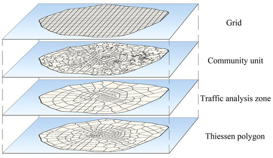
Figure 1.
Schematic diagram of zoning method for spatial unit.
2.2. Multicollinearity and Spatial Autocorrelation Test
2.2.1. Multicollinearity Test
Before building the regression model, it was necessary to carry out a multicollinearity test on the variables to avoid large bias in parameter estimation. Variance inflation factor (VIF) is often used as the measurement index [39]. The equation is as follows:
where R2 is the coefficient of determination in the regression equation. When VIF > 10, it is considered that there is multicollinearity, and this variable should be removed.
2.2.2. Spatial Autocorrelation Analysis
Different from the traditional linear regression model, the ride-hailing data and the data set of built environment factors adopted in this study have spatial attributes. Therefore, it was necessary to conduct spatial autocorrelation analysis for all variables before building the spatial econometric model [40]. Moran’s I test, as the most common spatial correlation test method, can reflect the spatial agglomeration effect of variables and the degree of influence on the spatial neighborhood attribute value [13]. The calculation equation is as follows:
where is the variance; n is the total number of spatial units; and are the observed values of spatial unit i and spatial unit j, respectively; is the mean value of each observed value; and is the spatial weight between the spatial units i and j. Moran’s I is between −1.0 and 1.0. When Moran’s I is greater than 0, it indicates that the variable has a positive spatial correlation, and the closer it is to 1.0, the stronger the spatial agglomeration effect is. When Moran’s I is less than 0, it indicates that the variable has a negative spatial correlation, and the closer it is to −1.0, the greater the spatial difference is. Moran’s I equaled 0, which means the variable was randomly distributed.
2.3. Regression Models
2.3.1. Ordinary Least-Squares Model
As a global regression method, the ordinary least-squares model mainly estimates non-spatial parameters to reflect the linear relationship between independent variables and dependent variables [41], as shown in Equation (5):
where is the ride-hailing pick-up ridership density of spatial unit i; is the intercept term; n is the total number of spatial units; is the regression coefficient of the k-th independent variable; is the k-th independent variable value of spatial unit i; and is the error term of spatial unit i.
2.3.2. Multi-scale Geographically Weighted Elastic Regression Model
Considering that the relationship between independent variable and dependent variable is affected by spatial location and spatial scale, Fotheringham et al. [42] proposed the MGWR model. Previous studies have proved that the MGWR model, as a local regression model, allows different independent variables to have independent optimal bandwidths to improve the goodness-of-fit of the regression model. In order to measure the elasticity of dependent variables to independent variables, natural logarithms of independent variables and dependent variables were taken on the basis of the MGWR model, and the improved MGWR model was referred to as MGWER, as shown in Equation (6).
where ln = natural log (i.e., log to the base e, and where e = 2.718); is the ride-hailing pick-up ridership density of spatial unit i; is the longitude and latitude coordinates of the centroid point of spatial unit i; is the intercept term of spatial unit i; n is the total number of spatial units; is the regression coefficient of the k-th independent variable of spatial unit i; bwk is the bandwidth of the k-th independent variable; is the k-th independent variable of spatial unit i; and is the error term of spatial unit i. Natural logarithms are taken for independent variables and dependent variables, indicating that every 1% change in , changes %. In this case, the slope coefficient measures the elasticity of the dependent variable to the independent variable [43].
3. Data and Variables
3.1. Study Area and Data Description
The study area is within the third ring road of downtown Chengdu, including Jinniu District, Qingyang District, Wuhou District, Jinjiang District, Chenghua District and Longquanyi District, with a total area of about 200 km2, as shown in Figure 2. The data includes the order data, urban road data, building outline data, POI data, housing price data and population data of ride-hailing in Chengdu, as shown in Table 2. We cleaned the data to check its completeness, accuracy and validity. We also removed duplicate values, missing values, outliers and data beyond the scope of the study.
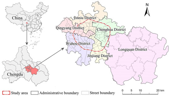
Figure 2.
Overview of the study area.
Table 2.
Data sources.
3.2. Dependent Variables
According to the start time of the order, the pick-up ridership is counted by hour, and its time distribution is shown in Figure 3. Considering that a large number of commuting trips on weekdays were concentrated in the morning and evening peak hours, and that the traffic demand and travel efficiency of these two periods most widely concerned travelers and researchers, the morning peak hours (07:00~11:00) and evening peak hours (16:00~20:00) of 5 consecutive working days were selected as the research period, and the average pick-ups in different periods were calculated. The pick-up density of a spatial unit in the morning and evening peak hours was taken as the dependent variable.
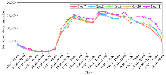
Figure 3.
Average hourly pick-up ridership of ride-hailing on weekdays.
3.3. Independent Variables
Cervero et al. [44] summarized the built environment as the “3Ds” dimensions, namely density, diversity and design, and explored the connection between the built environment “3Ds” and travel demand. Later, Ewing et al. [45] added destination accessibility and distance to transit to update the dimensions to the “5Ds”. In order to avoid the influence of data redundancy on the analysis results, the original 13 types of POI data were screened and reclassified into 4 types: residential POI, commercial POI, office POI and public service POI. The reclassification results are shown in Table 3. At the same time, the demand for ride-hailing is affected by the built environment and household income [27], the average housing price is introduced as a socio-economic attribute to measure residents’ income level [46] and the data set of built environment factors was constructed by combining the “5Ds” index of the built environment, as shown in Table 4.
Table 3.
Reclassification results of POI data.
Table 4.
Description of built environment factor data sets.
4. Results and Discussion
4.1. Multicollinearity and Spatial Autocorrelation Results
The multicollinearity test and spatial autocorrelation analysis were carried out for all variables under four spatial unit divisions: grid, community unit, TAZ and Thiessen polygon. The results showed that the VIF values of all independent variables were less than 10, indicating that there were not strong correlations between the selected variables. The road density showed significant spatial clustered distribution under community unit, TAZ and Thiessen polygon, while the bus station density showed significant spatial clustered distribution under 400 m and 1000 m grid and community unit. For a spatial unit division method, built environment variables with insignificant clustered distribution were eliminated during the construction of the MGWER model.
4.2. Spatial Unit of the Optimal Goodness-of-Fit Model
When the spatial cell grid scale is small, the number of cells becomes large, which leads to a significant increase in the calculation time of the MGWR model, leading to problems such as difficult convergence of regression results and poor fitting effect. Moreover, it is difficult for this regression-solving procedure to converge to a satisfactory result [30,42], which is not conducive to the determination of the optimal spatial unit and the application of the proposed method. Therefore, the OLS model was selected to compare the goodness-of-fit of linear models, corresponding to different spatial units to determine the optimal spatial unit. The coefficient of determination R2, adjusted coefficient of determination (Adj. R2), Akaike information criterion (AICc), and residual square sum (RSS) were used to compare the goodness-of-fit of regression models. The higher the coefficient of determination is, the better the fitting effect of the regression model is. The lower the AICc and RSS are, the better the fitting effect is [48]. By comparing the results of the OLS models of different spatial units (shown in Table 5), the morning and evening peak hours models under community unit division had the highest goodness-of-fit and relatively low model errors. The determination coefficient R2 of the OLS model was 0.757 in the morning peak hours and 0.752 in the evening peak hours, which improved the accuracy of the model compared with related research into ride-hailing [27]. Therefore, the relationship between built environment and demand for ride-hailing can be better explained by using community units as the optimal spatial units. The results of spatial autocorrelation shows that Moran’s I of all variables is greater than 0, p-value is less than 0.01 and Z-score is greater than 2.58, which proves that all variables were spatially clustered. The MGWR model can be used to further explore the elastic relationship between built environment and demand for ride-hailing and its spatial heterogeneity.
Table 5.
OLS model results of different spatial units.
4.3. Descriptive Statistics of Variables under Community Unit Division
Under the division of community units, the descriptive statistical results of variables are shown in Table 6. It can be seen that due to the different dimensions of each built environment factor, the numerical values of its statistical results are quite different. The density distribution of ride-hailing pick-up ridership in the morning and evening peak hours is shown in Figure 4. It can be seen that the density of ride-hailing pick-up ridership in the morning and evening peak hours have a similar spatial distribution. On the whole, it gradually decreases from the urban center to the periphery, and in some community units, the vehicle density in the evening peak hours was higher than that in the morning peak hours.
Table 6.
Descriptive statistics of variables.
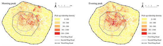
Figure 4.
Spatial distribution of pick-up ridership density of ride-hailing.
4.4. Optimal Bandwidth and Scale Effect of Built Environment Variables
To explain the elastic relationship between built environment and demand for ride-hailing, we added 1 to the values of both the independent and dependent variables and carried out logarithmic transformation before constructing the MGWER model. The relative influence of built environment on ridership demand for ride-hailing was measured using the elastic regression coefficient.
As an important parameter of the spatial regression model, bandwidth represents the number of adjacent community units required in parameter estimation, and is used to describe the scale difference between regression coefficients and the spatial influence range of each variable [49]. Table 7 shows the optimal bandwidth of each variable and spatial scale in the MGWER model in the morning and evening peak hours. The number of community units (that is, the total sample size) was 368. According to the optimal bandwidth results of each variable relative to the total sample size, the variables were divided into local, regional and global scales. The results show that the bandwidth of the average housing price in the morning and evening peak ranges from 45 to 90, and the bandwidth is relatively small, indicating that this variable affects the demand for ride-hailing on a local scale, and is sensitive to the impact of location, so it is defined as a local scale variable; the bandwidth of land-use mix entropy in the morning and evening peaks is 168, indicating that this variable has a relatively large spatial scale, we define it as a regional scale variable; the bandwidths of the floor area ratio, parking lot density, residential POI density, public service POI density and the distance to the nearest subway station in morning and evening peaks are all 367, covering almost the whole area within the Third Ring Road of Chengdu, indicating that the impact of these variables on demand for ride-hailing basically does not change with the change of spatial location. We defined it as a global-scale variable. In addition, the bandwidths of population density, commercial POI density, office POI density, road density, distance to CBD and bus stop density are greatly affected by time, showing different spatial characteristics in the morning and evening peaks.
Table 7.
Optimal bandwidth of variables and spatial scale of MGWER model in the morning and evening peak hours.
4.5. Influence Degree of built Environment Variables
The elastic coefficient of the MGWER model can reflect the relative influence of built environment on demand for ride-hailing. Table 8 shows the summary statistics of elastic coefficient of each variable in MGWER model. It includes the mean, minimum and maximum values of the elastic coefficients of the built environment variables, as well as the percentage of community units that are statistically significant based on the t-test at the 99% confidence level, the percentage of community units with positive coefficients, and the percentage of community units with negative coefficients. Floor area ratio and parking lot density have a significant positive impact on each community unit in the morning and evening peak hours, indicating that in the global scope, the higher the floor area ratio or the more the number of parking lots, the greater demand for ride-hailing. Residential POI density and distance to subway station were not significant influencing factors in the morning and evening peak hours, suggesting that these variables cannot well explain changes in demand for ride-hailing. The elasticity estimates of commercial POI density, public service POI density and land-use mix entropy have similar spatial distribution characteristics in the morning peak hours, and are significant and positive for each community unit. However, the elastic estimates of these variables differ greatly in the evening peak hours. The elastic coefficients of commercial POI density were significantly positive only in 9% of community units, the elastic coefficients of land-use mix entropy were significantly negative only in 16% of community units and the elastic coefficients of public service POI density were not significant in the evening peak hours. The results show that the built environment has different effects on demand for ride-hailing at different time periods.
Table 8.
Results statistics of elastic coefficients of variables of MGWER model.
In order to explore the main built environment factors affecting the demand for ride-hailing, this paper calculates the average elasticity coefficients of positive coefficients and significant negative coefficients, respectively. The influence of built environment variables on demand for ride-hailing was compared by the absolute value of elastic coefficients. The comparison of elasticity of variables in the MGWER model was presented in the form of a histogram, as shown in Figure 5. The elasticity of floor area ratio, parking lot density, commercial POI density and bus stop density in the morning and evening peak hours was positively correlated with demand for ride-hailing. However, the elasticity of population density, office POI density, land-use mix entropy, road density, distance to CBD and average housing price had significant differences in the morning and evening peak hours. For example, the elasticity of office POI density was negative in morning peak hours and positive in evening peak hours, indicating that the increase of office facilities can reduce the demand for ride-hailing in morning peak hours, while the demand for ride-hailing in evening peak hours will be increased. In the positive elasticity results, the density of commercial POI had the greatest impact on demand for ride-hailing, with the elasticity coefficient of 0.489 in the morning peak hours and 0.285 in the evening peak hours. It can be interpreted that for every 1% increase in commercial facilities in the area, the density of pick-up ridership of ride-hailing in morning peak hours will increase by 0.489% (Figure 5a), and the density of pick-up ridership of ride-hailing during evening peak hours will increase by 0.285% (Figure 5c). In the negative elasticity results, the distance to CBD has the greatest influence on demand for ride-hailing, and the elasticity coefficients of morning and evening peak hours are −0.284 and −0.219, respectively. It can be interpreted that for every 1% increase in the distance from the area to CBD, the density of pick-up ridership of ride-hailing in the morning and evening peak hours will decrease by 0.284% (Figure 5b) and 0.219% (Figure 5d), respectively.
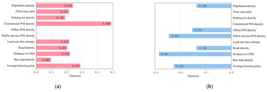
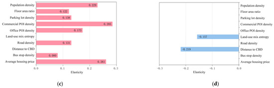
Figure 5.
Comparison of elasticity of variables: (a) positive elastic results of morning peak hours model; (b) negative elastic results of morning peak hours model; (c) positive elastic results of evening peak hours model; (d) negative elastic results of evening peak hours model.
According to the order of influence degree of elasticity of the built environment from high to low, the factors of built environment with positive influence in morning peak hours are as follows: commercial POI density, average housing price, population density, distance to CBD, land-use mix entropy, floor area ratio, road density, parking lot density and bus stop density. The factors of built environment with a negative influence are as follows: distance to CBD, public service POI density, average housing price, office POI density, road density and population density. The built environment factors that have a positive impact on the evening peak hours are as follows: commercial POI density, average housing price, population density, office POI density, parking lot density, road density, floor area ratio and bus stop density. The negative factors of built environment are distance to CBD and land-use mix entropy. Wang et al. [27] established the ride-hailing trip generation model with a grid size of 200 m. They concluded that numbers of restaurants and numbers of retail outlets have the greatest impact on ride-hailing trip generation, and this finding is similar to our results. In this paper, restaurant and retail factors belong to the same category as business POI density. Wang et al. found that the impact of floor area ratio is higher than that of population density and average housing price, which is different from the research results in this paper; this may be due to the selection of different independent variables and different zoning methods.
After sorting the above results, it can be seen that: (1) for the morning peak hours, the built environment factors with positive impacts are ranked as follows: commercial POI density > average house price > population density > distance to CBD > land-use mix entropy > floor area ratio > road density > parking lot density > bus stop density, and the built environment factors with negative impacts are ranked as follows: distance to CBD > public service POI density > average housing price > office POI density > road density > population density; (2) for the evening peak hours, the built environment factors with positive impacts are ranked as follows: commercial POI density > average housing price > population density > office POI density > parking lot density > road density > floor area ratio > bus stop density, and the built environment factors with negative impacts are ranked as follows: distance to CBD > land-use mix entropy.
4.6. Spatial Heterogeneity of Elasticity Coefficients
Figure 6 shows the spatial distribution of the elasticity coefficient of the built environment variables of the MGWER model. A positive elasticity coefficient indicates that the variable is positively correlated with demand for ride-hailing, which is represented in red. A negative elasticity coefficient indicates that the variable is negatively correlated with demand for ride-hailing, which is represented in blue. The darker the color, the greater the relative influence on ride-hailing ridership.
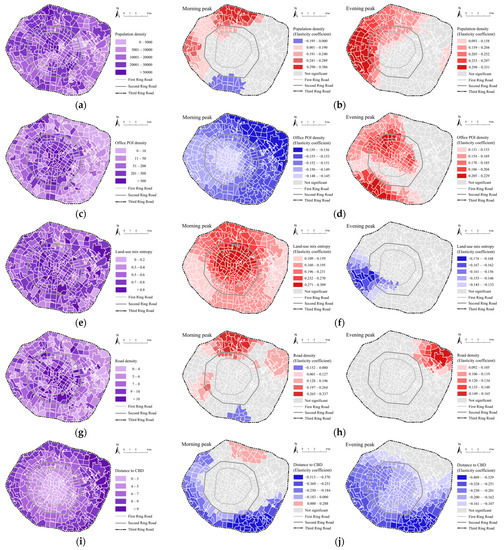
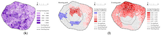
Figure 6.
Spatial distribution of built environment variables and elasticity coefficient result of MGWER model: (a) population density; (b) elastic coefficient of population density; (c) office POI density; (d) elastic coefficient of office POI density; (e) land-use mix entropy; (f) elastic coefficient of land-use mix entropy; (g) road density; (h) elasticity coefficient of road density; (i) distance to CBD; (j) elastic coefficient of distance to CBD; (k) average housing price; (l) elastic coefficient of average housing price.
Figure 6a shows the population density distribution of the community units. In general, areas with a large population will generate more travel demand [23]. Figure 6b shows the distribution of the elasticity coefficient of population density. In the western and northern areas outside the scope of the First Ring Road, there is a significant positive relationship between population density and demand for ride-hailing. The areas with high demand for ride-hailing in the morning peak hours are mainly concentrated in the north of the Second Ring Road and the areas with high demand for ride-hailing in the evening peak hours are mainly concentrated in the west of the Second Ring Road. It is worth noting that there is a weak negative correlation between population density and demand for ride-hailing in the morning peak hours in the south of the Second Ring Road. It can be seen from Figure 6a that the population density in this area is relatively high, but there is no more demand for ride-hailing. A possible reason is that the proportion of office facilities and public service facilities in this area is relatively large, and there are two large-scale hospitals in this area. In the morning peak hours, a large number of people travel to the region as a destination, and a small number of people use it as a starting point. As a result, there is relatively little demand for ride-hailing in this region.
Figure 6c shows that office facilities are mainly concentrated in the central area of the city. It can be seen from Figure 6d that the elasticity coefficient of office POI density varies greatly in the morning and evening peak hours. Office POI density in the morning peak hours is significant in all community units and is negatively correlated with ride-hailing ridership, which has the greatest impact in the northwest of the research area. The reason is that in an area with dense office facilities, more people come to work in the morning peak hours, resulting in less demand for ride-hailing. In contrast, office POI density in the evening peak hours is positively correlated with ride-hailing pick-up ridership and is mainly concentrated in the central part of the city and the southwest area outside the scope of the Second Ring Road. The possible reason is that there are a large number of people who need to return to their residence from their workplace and the areas with high office facility density will generate more demand for ride-hailing [16]. This is especially apparent in the southwest of the city with low office facility density, but the impact on demand for ride-hailing is large, indicating that increasing office facilities in this area can effectively increase demand for ride-hailing.
Figure 6e shows the spatial distribution of land-use mix entropy. The land-use mix entropy represents the mixed degree of land-use functions and the abundance of facilities in the region [50]. The elastic coefficient of land-use mix entropy is shown in Figure 6f. In the morning peak hours model, the land-use mix entropy is significant in all community units of the study area, while in the evening peak hours model, the land-use mix entropy is only significant in a small range in the southwest of the city. The results show that there is a strong positive correlation between land-use mix entropy and demand for ride-hailing in the morning peak hours, and the closer to the city center, the greater the impact. Generally, areas with high diversity have relatively diverse service facilities, which can attract more people and generate more traffic demand than other areas. However, in the evening peak hours, the land-use mix entropy is negatively correlated with demand for ride-hailing, which may be due to the fact that residents tend to consume nearby in the evening [51], resulting in less demand for ride-hailing than in other areas.
Generally, high-road-density areas will generate more traffic demand [52]. Figure 6g shows the spatial distribution of road density. It can be seen that the areas with high road density are mainly concentrated within the Second Ring Road. Figure 6h shows the distribution of the elasticity coefficient of road density, and the areas significantly affected by road density are mainly distributed between the Second Ring Road and the Third Ring Road. On the whole, the road density in most of this area has a positive impact on the demand for ride-hailing, which may be due to the higher population density and more traffic volume in areas with higher road density [26]. However, there are also exceptions. In the morning peak hours, the road density in the south of the city has a weak negative correlation with demand for ride-hailing. Although the road density in this area is small, because the Chengdu South Railway Station is located in this area, there is a high flow of people and demand for ride-hailing.
Figure 6i shows the distance from each community unit to the CBD, which is usually used to reflect the commercial proximity of each region [23]. Figure 6j shows the distribution of the elasticity coefficient of the distance to the CBD. For most regions where demand for ride-hailing is significantly affected by distance to the CBD, the distance to the CBD has a negative effect on the demand for ride-hailing, and the southeast of the research area is the place with the greatest impact of this variable. A possible reason is that the farther away an area is from the city center, the more often it is accompanied by long-distance commuting [53]. Because of the high cost of long-distance travel of ride-hailing, more passengers will choose to travel by bus or subway. However, in the area north of the Second Ring Road in the morning peak hours, the distance to the CBD is positively correlated with the demand for ride-hailing; that is, the demand for ride-hailing in the area far from the downtown is also large. The possible reason is that the area is close to Chengdu North Railway Station and the long-distance bus station, which generates more demand for ride-hailing.
As a social and economic attribute, housing price can reflect the actual consumption capacity of residents to a certain extent [15], which is very important to explain demand for ride-hailing. Figure 6k shows the spatial distribution of the average housing price, showing a trend of low in the northeast and high in the southwest. Figure 6l shows the distribution of elasticity coefficient of the average housing price. It can be seen that the impact of the average housing price on demand for ride-hailing is more complex in space. It is generally believed that high-income groups are more willing to pay for ride-hailing services. However, in the western and southern regions of the city during the morning peak hours, the average housing price is negatively correlated with the impact of demand for ride-hailing. It can be seen from Figure 6k that the average housing price in this area is generally high, including some private villas, and some high-income people may prefer to drive private cars instead of using ride-hailing services.
5. Conclusions
This paper formulated the MGWER model to analyze the effects of built environment factors on demand for ride-hailing. Considering the scale effect and zoning effect in MAUP, this paper aggregates the built environment “5Ds” factors and pick-up ridership of ride-hailing into the spatial units according to four zoning methods, which are grid scale, traffic analysis zone, Thiessen polygon and community unit. The community unit was determined as the optimal spatial unit by comparing the goodness-of-fit of the global OLS regression model. This process of finding the optimal scale and zoning method is crucial for the aggregate analysis of geographical big data, and should be carried out before the regression model of built environment and ride-hailing ridership is constructed. The framework and approach proposed in this paper can also be applied to other analyses of geographical big data. We integrated logarithmic dependent variables and independent variables into the MGWR model and put forward the MGWER model. This study focuses on the elastic relationship between the built environment and demand for ride-hailing, and compares the influence degree and spatial heterogeneity of different built environment variables on the demand for ride-hailing. We ranked the elastic impact of each built environment factor, and the results showed that the built environment factor with the greatest positive impact during peak hours was the density of commercial POI density, while the built environment factor with the greatest negative impact was the distance to CBD. Meanwhile, the elastic relationship between the built environment and the demand for ride-hailing services showed spatial heterogeneity and was influenced by different peak periods. The impact of six built environment factors, including population density, office POI density, land-use mix entropy, road density, distance to CBD and average housing price, varied significantly at different locations. The result of elasticity coefficient reflects the effect of 1% change of an independent variable on the percentage change of a dependent variable. Compared with linear regression models, such as OLS and MGWR, it more clearly and directly expresses the important impact of built environment variables on ride-hailing ridership.
This study explores the relationship between the built environment and demand for ride-hailing, which can provide reference for the operation and management of ride-hailing and urban planning decision-making. Urban planners can make a preliminary prediction of the demand for ride-hailing passenger flow according to the built environment, and on this basis, they can set up ride-hailing stops in areas with high demand, so as to reduce the impact of ride-hailing on road traffic during peak periods. For ride-hailing operators, the demand for ride-hailing can be predicted according to the built environment factors by using the MGWER model, which will be conducive to the scheduling optimization plan of ride-hailing. When adjusting the demand for ride-hailing of the whole city, policy-makers should focus on the built environment variables with a high degree of elastic influence and make scientific decisions, which is conducive to achieving the expected goals. For community service departments, strategies and planning schemes for community renewal of built environment should be formulated according to the spatial heterogeneity impacts of built environment variables. For example, within the First Ring Road of the city, it is possible to reduce the demand for ride-hailing in the region by updating the built environment to decrease the variables with positive impact or increase the variables with the negative impact on ride-hailing ridership, so as to alleviate the traffic congestion caused by the concentration of ride-hailing trips. For areas outside the scope of the First Ring Road, it is suggested to encourage ride-hailing and other shared travel modes to improve the traffic accessibility of the outer areas of the city center.
This study has the following limitations: (1) there are cases of people not being able to order a ride-hailing service during peak periods, which may underestimate the actual demand for ride-hailing services; (2) further research needs to be extended to weekend days and holidays, and consider the drop-off ridership of ride-hailing to reveal the relationship between the built environment and demand for ride-hailing; (3) due to the limitations of the MGWR model itself, the excessive sample size will lead to a sharp increase in the time cost of the model, so this study used the global OLS model to determine the optimal space unit, which is expected to improve with the progress of the model in the future; (4) the research results are only applicable to Chengdu, but it is not known whether different cities have similar results, so we need to analyze more cities to verify the accuracy of the results in the future.
Author Contributions
Conceptualization, Z.W. X.G. and N.C.; data curation, X.G.; methodology, Z.W., N.C. and X.G.; software, X.G., Z.W. and S.L.; writing—original draft, Z.W., X.G. and Y.Z.; writing—review and editing, Z.W., X.G. and Y.Z. All authors have read and agreed to the published version of the manuscript.
Funding
This research was supported by Hebei Social Science Development Research Project, China (grant No. 20210201407).
Institutional Review Board Statement
Not applicable.
Informed Consent Statement
Not applicable.
Data Availability Statement
The data used in this study are available from the corresponding author upon reasonable request.
Conflicts of Interest
The authors declare no conflict of interest.
References
- Standing, C.; Standing, S.; Biermann, S. The implications of the sharing economy for transport. Transp. Rev. 2019, 39, 226–242. [Google Scholar] [CrossRef]
- Sui, Y.; Zhang, H.; Song, X.; Shao, F.; Yu, X.; Shibasaki, R.; Sun, R.; Yuan, M.; Wang, C.; Li, S.; et al. GPS data in urban online ride-hailing: A comparative analysis on fuel consumption and emissions. J. Clean. Prod. 2019, 227, 495–505. [Google Scholar] [CrossRef]
- Machado, C.A.S.; De Salles Hue, N.P.M.; Berssaneti, F.T.; Quintanilha, J.A. An overview of shared mobility. Sustainability 2018, 10, 4342. [Google Scholar] [CrossRef]
- Jin, S.T.; Kong, H.; Wu, R.; Sui, D.Z. Ridesourcing, the sharing economy, and the future of cities. Cities 2018, 76, 96–104. [Google Scholar] [CrossRef]
- Handy, S.L.; Boarnet, M.G.; Ewing, R.; Killingsworth, R.E. How the built environment affects physical activity: Views from urban planning. Am. J. Prev. Med. 2002, 23, 64–73. [Google Scholar] [CrossRef] [PubMed]
- Zhou, M.; Bai, Z.; Gao, X.; Wang, X.; Zhao, C. Excavation of the spatio-temporal pattern of passenger travel in Haikou city. Sci. Surv. Mapp. 2021, 46, 117–184. [Google Scholar]
- Wang, S.; Wang, J.; Li, W.; Fan, J.; Liu, M. Revealing the influence mechanism of urban built environment on online car-hailing travel considering orientation entropy of street network. Discret. Dyn. Nat. Soc. 2022, 2022, 3888800. [Google Scholar] [CrossRef]
- Lu, X.; Ma, C.; Qiao, Y. Short-term demand forecasting for online car-hailing using ConvLSTM networks. Phys. A Stat. Mech. Its Appl. 2021, 570, 125838. [Google Scholar] [CrossRef]
- Wang, B.; Zhu, R.; Zhang, S.; Zhao, Z.; Yang, X.; Wang, G. PPVF: A novel framework for supporting path planning over carpooling. IEEE Access 2019, 7, 10627–10643. [Google Scholar] [CrossRef]
- Sun, D.; Zhang, K.; Shen, S. Analyzing spatiotemporal traffic line source emissions based on massive didi online car-hailing service data. Transp. Res. Part D 2018, 62, 699–714. [Google Scholar] [CrossRef]
- Ren, Q.; Jin, L.; Wu, L.; Su, L. Research on China’s online booking regulations and counter measures. J. Chongqing Jiaotong Univ. (Soc. Sci. Ed.) 2017, 17, 38–41. [Google Scholar]
- Lyu, T.; Wang, P.; Gao, Y.; Wang, Y. Research on the big data of traditional taxi and online car-hailing: A systematic review. J. Traffic Transp. Eng. (Engl. Ed.) 2021, 8, 1–34. [Google Scholar] [CrossRef]
- Yu, L.; Xie, B.; Zhang, K.; Sun, Y. Impacts of built environments on car-hailing commuting in job-housing locations. J. Transp. Inf. Saf. 2019, 37, 149–155. [Google Scholar]
- Nam, D.; Hyun, K.; Kim, H.; Ahn, K.; Jayakrishnan, R. Analysis of grid cell-based taxi ridership with large-scale GPS data. Transp. Res. Rec. J. Transp. Res. Board 2016, 2544, 131–140. [Google Scholar] [CrossRef]
- Chen, C.; Feng, T.; Ding, C.; Yu, B.; Yao, B. Examining the spatial-temporal relationship between urban built environment and taxi ridership: Results of a semi-parametric GWPR model. J. Transp. Geogr. 2021, 96, 103172. [Google Scholar] [CrossRef]
- Li, T.; Jing, P.; Li, L.; Sun, D.; Yan, W. Revealing the varying impact of urban built environment on online car-hailing travel in spatio-temporal dimension: An exploratory analysis in Chengdu, China. Sustainability 2019, 11, 1336. [Google Scholar] [CrossRef]
- Weng, J.; He, H.; Wang, Y.; Zhang, K.; Qian, H. Regional taxi travel demand influencing model based on geographical weighted regression. Transp. Res. 2020, 6, 28–38. [Google Scholar]
- Shen, J.; Liu, X.; Chen, M. Discovering spatial and temporal patterns from taxi-based Floating Car Data: A case study from Nanjing. GIScience Remote Sens. 2017, 54, 617–638. [Google Scholar] [CrossRef]
- Kolaczyk, E.D.; Huang, H. Multiscale statistical models for hierarchical spatial aggregation. Geogr. Anal. 2001, 33, 95–118. [Google Scholar] [CrossRef]
- Zhou, X.; Yeh, A.G.O. Understanding the modifiable areal unit problem and identifying appropriate spatial unit in jobs–housing balance and employment self-containment using big data. Transportation 2020, 48, 1267–1283. [Google Scholar] [CrossRef]
- Wang, Z.; Song, J.; Zhang, Y.; Li, S.; Jia, J.; Song, C. Spatial heterogeneity analysis for influencing factors of outbound ridership of subway stations considering the optimal scale range of “7D” built environments. Sustainability 2022, 14, 16314. [Google Scholar] [CrossRef]
- Zhao, G.; Li, Z.; Shang, Y.; Yang, M. How does the urban built environment affect online car-hailing ridership intensity among different scales? Int. J. Environ. Res. Public Health 2022, 19, 5325. [Google Scholar] [CrossRef] [PubMed]
- Yang, Z.; Franz, M.L.; Zhu, S.; Mahmoudi, J.; Nasri, A.; Zhang, L. Analysis of Washington, DC taxi demand using GPS and land-use data. J. Transp. Geogr. 2018, 66, 35–44. [Google Scholar] [CrossRef]
- Zhang, B.; Chen, S.; Ma, Y.; Li, T.; Tang, K. Analysis on spatiotemporal urban mobility based on online car-hailing data. J. Transp. Geogr. 2020, 82, 102568. [Google Scholar] [CrossRef]
- Bi, H.; Ye, Z.; Wang, C.; Chen, E.; Li, Y.; Shao, X. How built environment impacts online car-hailing ridership. Transp. Res. Rec. J. Transp. Res. Board 2020, 2674, 745–760. [Google Scholar] [CrossRef]
- Qian, X.; Ukkusuri, S.V. Spatial variation of the urban taxi ridership using GPS data. Appl. Geogr. 2015, 59, 31–42. [Google Scholar] [CrossRef]
- Wang, S.; Noland, R.B. Variation in ride-hailing trips in Chengdu, China. Transp. Res. Part D Transp. Environ. 2021, 90, 102596. [Google Scholar] [CrossRef]
- Zhang, X.; Huang, B.; Zhu, S. Spatiotemporal influence of urban environment on taxi ridership using geographically and temporally weighted regression. ISPRS Int. J. Geo-Inf. 2019, 8, 23. [Google Scholar] [CrossRef]
- Gladhill, K.; Monsere, C.M. Exploring traffic safety and urban form in Portland, Oregon. Transp. Res. Rec. J. Transp. Res. Board 2012, 2318, 63–74. [Google Scholar] [CrossRef]
- Shen, T.; Yu, H.; Zhou, L.; Gu, H.; He, H. On hedonic price of second-hand houses in Beijing based on multi-scale geographically weighted regression: Scale law of spatial heterogeneity. Econ. Geogr. 2020, 40, 75–83. [Google Scholar]
- Lao, X.; Gu, H. Unveiling various spatial patterns of determinants of hukou transfer intentions in China: A multi-scale geographically weighted regression approach. Growth Chang. 2020, 51, 1860–1876. [Google Scholar] [CrossRef]
- Zhou, L.; Wu, T.; Jiang, G.; Zhang, J.; Pu, L.; Xu, F.; Xie, X. Spatial heterogeneity of PM2.5 concentration in response to land use/cover conversion in the Yangtze River delta region. Environ. Sci. 2022, 43, 1201–1211. [Google Scholar]
- Maiti, A.; Zhang, Q.; Sannigrahi, S.; Pramanik, S.; Chakraborti, S.; Cerda, A.; Pilla, F. Exploring spatiotemporal effects of the driving factors on COVID-19 incidences in the contiguous United States. Sustain. Cities Soc. 2021, 68, 102784. [Google Scholar] [CrossRef] [PubMed]
- Tomal, M. Exploring the meso-determinants of apartment prices in Polish counties using spatial autoregressive multiscale geographically weighted regression. Appl. Econ. Lett. 2022, 29, 822–830. [Google Scholar] [CrossRef]
- Qu, X.; Zhu, X.; Xiao, X.; Wu, H.; Guo, B.; Li, D. Exploring the influences of point-of-interest on traffic crashes during weekdays and weekends via multi-scale geographically weighted regression. ISPRS Int. J. Geo-Inf. 2021, 10, 791. [Google Scholar] [CrossRef]
- Gao, D.; Xu, Q.; Chen, P.; Hu, J.; Zhu, Y. Spatial characteristics of urban rail transit passenger flows and fine-scale built environment. J. Transp. Syst. Eng. Inf. Technol. 2021, 21, 25–32. [Google Scholar]
- Ji, H.; Cai, Z.; Jiang, L.; Li, G.; Li, B. Analysis of spatial inequality in taxi ride and its relationship with population structure. Geomat. Inf. Sci. Wuhan Univ. 2021, 46, 766–776. [Google Scholar]
- Zhao, M.; Liu, S.; Qi, W. Spatial identification and scale effects of floating population agglomerations at the community scale: A case study of Beijing. Geogr. Res. 2018, 37, 1208–1222. [Google Scholar]
- Zhang, L.; Yang, Y.; Liang, X. The diagnostic approach of multicollinearity in geographically weighted regression model. Geomat. Spat. Inf. Technol. 2017, 40, 28–31. [Google Scholar]
- Goodchild, M.F. Geographical data modeling. Comput. Geosci. 1992, 18, 401–408. [Google Scholar] [CrossRef]
- Zhou, X.; Hao, H.; Ye, X.; Qin, Y.; Ma, X. A spatial-temporal analysis of regional economic inequality in Yellow River Valley. Hum. Geogr. 2016, 31, 119–125. [Google Scholar]
- Fotheringham, A.S.; Yang, W.; Kang, W. Multiscale geographically weighted regression (MGWR). Ann. Am. Assoc. Geogr. 2017, 107, 1247–1265. [Google Scholar] [CrossRef]
- Gujarati, D.N.; Porter, D.C. Basic Econometrics, 5th ed.; McGraw-Hill/Irwin: New York, NY, USA, 2009; pp. 159–160. [Google Scholar]
- Cervero, R.; Kockelman, K. Travel demand and the 3Ds: Density, diversity, and design. Transp. Res. Part D: Transp. Environ. 1997, 2, 199–219. [Google Scholar] [CrossRef]
- Ewing, R.; Cervero, R. Travel and the built environment: A synthesis. Transportation Research Record. J. Transp. Res. Board 2001, 1780, 87–114. [Google Scholar] [CrossRef]
- Wang, D.; Cao, X. Impacts of the built environment on activity-travel behavior: Are there differences between public and private housing residents in Hong Kong? Transp. Res. Part A 2017, 103, 25–35. [Google Scholar] [CrossRef]
- Frank, L.D.; Andresen, M.A.; Schmid, T.L. Obesity relationships with community design, physical activity, and time spent in cars. Am. J. Prev. Med. 2004, 27, 87–96. [Google Scholar] [CrossRef]
- Sugiura, N. Further analysts of the data by akaike’ s information criterion and the finite corrections. Commun. Stat. Theory Methods 1978, 7, 13–26. [Google Scholar] [CrossRef]
- Yu, H.; Fotheringham, A.S.; Li, Z.; Oshan, T.; Kang, W.; Wolf, L.J. Inference in multiscale geographically weighted regression. Geogr. Anal. 2020, 52, 87–106. [Google Scholar] [CrossRef]
- Li, Q.; Peng, J.; Yang, H. Research on relationship analysis between passenger flow characteristics of rail transit stations and built environment of different station areas in Wuhan. J. Geo-Inf. Sci. 2021, 23, 1246–1258. [Google Scholar]
- Xie, W.; Zhou, S. The spatial-temporal-nonstationary effect of built-environment on taxi demand. Mod. Urban Res. 2018, 33, 22–29. [Google Scholar]
- Tu, W.; Cao, R.; Yue, Y.; Zhou, B.; Li, Q.; Li, Q. Spatial variations in urban public ridership derived from GPS trajectories and smart card data. J. Transp. Geogr. 2018, 69, 45–57. [Google Scholar] [CrossRef]
- An, R.; Wu, Z.; Tong, Z.; Qin, S.; Zhu, Y.; Liu, Y. How the built environment promotes public transportation in Wuhan: A multiscale geographically weighted regression analysis. Travel Behav. Soc. 2022, 29, 186–199. [Google Scholar] [CrossRef]


Disclaimer/Publisher’s Note: The statements, opinions and data contained in all publications are solely those of the individual author(s) and contributor(s) and not of MDPI and/or the editor(s). MDPI and/or the editor(s) disclaim responsibility for any injury to people or property resulting from any ideas, methods, instructions or products referred to in the content. |
© 2023 by the authors. Licensee MDPI, Basel, Switzerland. This article is an open access article distributed under the terms and conditions of the Creative Commons Attribution (CC BY) license (https://creativecommons.org/licenses/by/4.0/).