Optimal Allocation and Sizing of Distributed Generation Using Interval Power Flow

Abstract

Modern distribution systems and microgrids must deal with high levels of uncertainty in their planning and operation. These uncertainties are mainly due to variations in loads and distributed generation (DG) introduced by new technologies. This scenario brings new challenges to planners and system operators that need new tools to perform more assertive analyses of the grid state. This paper presents an optimization methodology capable of considering uncertainties in the optimal allocation and sizing problem of DG in distribution networks. The proposed methodology uses an interval power flow (IPF) that adds uncertainties to the combinatorial optimization problem in charge of sizing and allocating DG units in the network. Two metaheuristics were implemented for comparative purposes, namely, symbiotic organism search (SOS) and particle swarm optimization (PSO). The proposed methodology was implemented in Python^® using as benchmark distribution systems the IEEE 33-bus and IEEE 69-bus test distribution networks. The objective function consists of minimizing technical losses and regulating network voltage levels. The results obtained from the proposed IPF on the tested networks are compatible with those obtained by the PPF, thus evidencing the robustness and applicability of the proposed method. For the solution of the optimization problem, the SOS metaheuristic proved to be robust, since it was able to find the best solutions (lowest losses) while keeping voltage levels within the predetermined range. On the other hand, the PSO metaheuristic showed less satisfactory results, since for all test systems, the solutions found were of lower quality than the ones found by the SOS.

1. Introduction

Electric power systems (EPSs) play an important role in modern societies as they enable the use of technologies and supply electrical energy to industries and households. Nevertheless, their proper functioning can only be guaranteed if they have an adequate set of tools for their operation and planning. Among these studies, the most common analysis is the power flow (PF) in its AC and DC variants, which can be computed by using several widely known techniques [1,2]. Still, the biggest weakness of these studies is that the accuracy of their results is as good as the accuracy of the input data [3]. Power flow inaccuracy can be due to measurement errors, inaccurate forecasts, assumptions of limits on load, or scheduled outages [4].

The current political and economic landscape of the energy industry has increasingly encouraged the use of distributed energy resources (DERs), which include small-scale consumer-side generation, energy storage equipment, and demand response (DR) [5,6,7,8]. Thus, the role of consumers has been progressively changing, becoming more active. In this context, load models must adapt to characterize these new uncertainties [9]. Interval analysis can be seen as an effective tool for considering these uncertainties in PF problems. In this case, loads are modeled by a set of values varying linearly from the smallest to the largest possible value, and thus nodal voltages, power flows, and losses are calculated in an interval manner. This approach is known as interval power flow (IPF) [10,11,12,13].

Some mathematical tools are needed to calculate the IPF and ensure its convergence. This can be accomplished either by Newton’s interval method or Krawczyk’s method [14], which finds the interval solution of a system with a given tolerance. In [13], an optimal distribution planning model is proposed using IPF for uncertainty addition, where the interval results are used as merit functions in an optimization algorithm. Complementing IPF, interval mathematics are also used for uncertainty addition in problems such as state estimation and short-circuit calculation [15].

Another approach to adding uncertainty is the probabilistic power flow (PPF) [16,17,18]. In this case, loads are modeled by means of their density functions. Several research works have proposed mathematical models to solve this problem. Monte Carlo simulation (MCS) is the most widely used method for approaching a PPF. This method consists of solving several deterministic PF with random variations of their parameters based on their probability density functions, so if a large enough sample of results is obtained, a highly accurate result can be expected [19]. Probabilistic uncertainties can also be modeled by other methods, such as polynomial chaos expansion (PCE), which is able to work in a non-intrusive way and model random variables and stochastic processes with a high performance [20].

Table 1. Main characteristics of CPF, IPF, and PPF.

	Conventional PF	Interval PF	Probabilistic PF
Nature of input variables	Deterministic variables	Interval variables	Probability distribution functions
Mathematical model	Power balance equations with conventional mathematical operations	Power balance equations with interval mathematical operations	Conventional power balance equations considering the realizations of random variables
Solution approach	Newton–Raphson	Krawczyk method	A pre-determined number of simulations, each running a Newton–Raphson
Obtained solution	Unic solution	Interval form (interval ranges of the output data are not necessarily the same as those of the input data)	Probability distribution function (not necessarily the same as the one of the input data)

presents the main characteristics of conventional power flow (CPF), IPF, and PPF.

IPF has been shown to be an effective tool to deal with uncertainties. In [21], the authors implemented an IPF analysis considering interval power injections from wind farms with the aim of guaranteeing interval values of the grid variables for safe system operation. In [22], an affine arithmetic-based PF is proposed for the consideration of unscheduled regional power fluctuations. The authors in [23] proposed an IPF based on a multi-stage affine arithmetic to consider the uncertainty of loads and DG in an unbalanced network. In [24], a hybrid between interval and probabilistic power flow is proposed using an analytical clustering method. In this case, the uncertainties of random and interval variables are considered simultaneously. The authors in [25] proposed an IPF to generate optimal scenarios. In this approach, the interval uncertainties are considered with variable bounds, and the objective function is programmed to compute such bound. In [26], the authors proposed an IPF based on the Taylor inclusion function, while in [27] an IPF is proposed using the correlation of the uncertainties of the power injections. Other variants of the IPF are also proposed in [28,29].

Even though power flow accuracy has improved, the distribution planning problem involving the integration of DG is still complex. Therefore, several studies have also been devoted to current and power control in distribution networks with DG [30,31,32]. Grid connections for DG are significantly different from traditional centralized generator connections. Several factors must be analyzed for planning the connection of DG, such as the number of generating sources, their locations, and connection types, among others [33,34,35].

The installation of DG in non-optimal locations brings along a series of problems to the network, including problems with protection coordination, over-voltages, and also an increment on technical losses, therefore, having the opposite effect of the desired one [36,37,38]. Thus, using a method capable of selecting the best locations and preferable sizing in a complex distribution network represents a useful tool for planners.

The problem of allocation and sizing of DG consists of two steps that are solved together, the selection of the best locations for the installation of the generation and the choice of the maximum capacity of each generating unit [39]. This problem has been widely studied using a series of different objectives. Such objectives can be minimizing losses [40], improving voltage profile [41], minimizing investments and maintenance costs [42] improvement of system reliability indices [43], and spinning reserve increment [44]; furthermore, there are proposals that combine several of these objectives [45,46,47].

The optimal location and sizing of DG is a complex optimization problem that can be tackled by metaheuristic techniques such as genetic and evolutionary algorithms [48], particle swarm optimization [49], symbiotic organism search (SOS) [50], gray wolf optimizer [51], crow search algorithm [52], artificial ecosystem-based optimization [53], and hybrid methodologies [54]. Recently, SOS and particle swarm optimization (PSO) [55,56] have demonstrated to be effective when solving complex optimization problems. PSO and SOS are optimization methodologies based on the behavior of swarms and symbiotic organisms, respectively.

This paper presents a methodology for the optimal allocation and sizing of DG in distribution networks that takes into account the existing uncertainties in loads and generators. The proposed methodology is based on an IPF for adding uncertainties; furthermore, PSO and SOS are used for the optimization of generation in the grid; nonetheless, any other metaheuristic technique might be applied. One of the strengths of IPF is that uncertainties are considered through the percentage variation of the variables of interest; then, it is possible to incorporate the expertise of the network operator to determine the most appropriate ranges of variation of these variables and therefore, obtain more accurate modeling of the operation. Furthermore, due to its nature, the IPF features a reduced computational effort when compared to probabilistic approaches that require thousands of simulations. In this sense, the main contributions of this paper are as follows: (i) it presents a methodology capable of adding and evaluating uncertainties in the process of optimal DG siting and sizing in distribution systems, (ii) two metaheuristic techniques are implemented for assessing the performance of the proposed approach; namely, PSO and SOS, and (iii) an analysis of the convergence of both metaheuristics operating with interval values is carried out along with an evaluation of their performance under two different metrics.

2. Uncertainty Modeling

The uncertainty modeling was carried out following the IPF implemented by the authors in [57] and is summarized below.

Step 1: Use a deterministic power flow to compute the bus voltages of the test system. In this case, the input variables may be fixed at their deterministic values. Once this is done, the percentage variations in demand and their respective interval values can be calculated using Equations (1) and (2). In this case, ${Pc}_k^d$ and ${Qc}_k^d$ represent the deterministic values of the active and reactive loads at bus k, respectively. ${Pc}_k^i$ and ${Qc}_k^i$ are the interval values of the active and reactive loads and $\alpha$ represents the percentage variation of the demand.

$${Pc}_k^i={Pc}_k^d\left[1-\alpha ,1+\alpha \right]$$

(1)

$${Qc}_k^i={Qc}_k^d\left[1-\alpha ,1+\alpha \right]$$

(2)

Step 2: The expected values of the interval active and reactive power are calculated using Equations (3) and (4). In this case, $P_{{exp}_k}^i$ and $Q_{{exp}_k}^i$ are the interval active and interval reactive powers expected at bus k, while $P_{{exp}_k}^d$ and $Q_{{exp}_k}^d$ are the expected active and reactive power used in the deterministic power flow.

$$P_{{exp}_k}^i=P_{{exp}_k}^d-{Pc}_k^d+{Pc}_k^i$$

(3)

$$Q_{{exp}_k}^i=Q_{{exp}_k}^d-{Qc}_k^d+{Qc}_k^i$$

(4)

The interval mismatches for initializing magnitudes and angles of bus voltages are calculated as the difference between the interval powers and their deterministic values calculated at each bus. Then, the interval increments of the modules and angles of the bus voltages are calculated using the Jacobian matrix of the last iteration of the deterministic power flow. Thus, the interval magnitudes and angles of the bus voltages can be calculated using their deterministic results and the interval increments as detailed in [57].

Step 3: The interval active and reactive powers are calculated using Equations (5) and (6), where $∥\dot{V_k^i}∥$ and $∥\dot{V_m^i}∥$ are the magnitudes of the interval voltages at buses k and m, respectively. $G_{ij}$ and $B_{ij}$ are the real and imaginary components of the system admittance matrix ($Y_{ij}$) and ${\theta }_k^i$ and ${\theta }_m^i$ are the interval phase angles of the voltages at buses k and m, respectively. Finally, $P_{{calc}_k}^i$ and $Q_{{calc}_k}^i$ are the interval values of the active and reactive powers.

$$P_{{calc}_k}^i={∥\dot{V_k^i}∥}^2{G}_{kk}+∥\dot{V_k^i}∥\sum _{mϵ\mathsf{\Omega }k}^k∥\dot{V_m^i}∥\left(G_{km}cos\left({\theta }_k^i-{\theta }_m^i\right)+B_{km}sin\left({\theta }_k^i-{\theta }_m^i\right)\right)$$

(5)

$$Q_{{calc}_k}^i=-{∥\dot{V_k^i}∥}^2{B}_{kk}+∥\dot{V_k^i}∥\sum _{mϵ\mathsf{\Omega }k}^k∥\dot{V_m^i}∥\left(-B_{km}cos\left({\theta }_k^i-{\theta }_m^i\right)+G_{km}sin\left({\theta }_k^i-{\theta }_m^i\right)\right)$$

(6)

Then, the interval mismatches are recalculated using Equations (7) and (8).

$$\mathsf{\Delta }{P}_k^i=P_{{exp}_k}^i-P_{{calc}_k}^i$$

(7)

$$\mathsf{\Delta }{Q}_k^i=Q_{{exp}_k}^i-Q_{{calc}_k}^i$$

(8)

Step 4: Apply the Krawczyk operator and update the interval values of voltage angles and magnitudes using Equation (9).

$${\left[\begin{array}{c}{\theta }^i\\ V^i\end{array}\right]}^{h+1}=\left[\begin{array}{c}{\theta }^i\\ V^i\end{array}\right]\bigcap K\left(x^h,X^h\right)$$

(9)

Step 5: Check whether the largest variation in the radius of the variables between iterations is smaller than the specified tolerance, if yes, the interval power flow has converged, if not, return to step 4.

Step 6: Compute the desired interval electric output quantities, $L^i(V_k,{\theta }_k,V_m,{\theta }_m)$ using Equations (10) and (11).

$$\mathsf{\Delta }{L}^i=\left[\frac{\partial L^d}{\partial {\theta }_k}{X}_p+\frac{\partial L^d}{\partial V_k}{Y}_p+\frac{\partial L^d}{\partial {\theta }_m}{Z}_p+\frac{\partial L^d}{\partial V_m}{W}_p\right]{\left[\mathsf{\Delta }{P}^i\mathsf{\Delta }{Q}^i\right]}^t$$

(10)

$$L^i=L^d+\mathsf{\Delta }{L}^i$$

(11)

where $L^i$ and $L^d$ are, respectively, the interval and deterministic values of the output magnitude. $X_p$, $Y_p$, $Z_p$, and $W_p$ are the rows of the inverse Jacobian matrix evaluated after the convergence of the deterministic FP as shown in Equation (12).

$${[\dots \mathsf{\Delta }{\theta }_k^i\mathsf{\Delta }{V}_k^i\dots \mathsf{\Delta }{\theta }_m^i\mathsf{\Delta }{V}_m^i\dots ]}^t={[\dots X_p{Y}_p\dots Z_p{W}_p\dots ]}^t{\left[\mathsf{\Delta }{P}^i\mathsf{\Delta }{Q}^i\right]}^t$$

(12)

3. Optimal Location and Sizing of DG

Consumers and investors are those who usually decide on the location of new DG units based on their needs and resources. Nonetheless, the utility may provide incentives for the location of DG in specific places of the network that would render other benefits. The approach presented in this paper considers that the utility may decide on the location and sizing of new DG units within the network. The objective function is the minimization of total active power losses with the sitting and sizing of DG as decision variables. Furthermore, an IPF is used to introduce uncertainty to the problem.

3.1. Mathematical Modeling

DG allocation in non-optimal locations may cause technical issues such as an increment in power losses and problems in protection coordination schemes. Therefore, it is important to have an approach capable of selecting the best locations and preferable sizing of DG in distribution networks [58].

Metaheuristic techniques are optimization tools better suited to handle combinatorial, non-convex optimization problems than classic approximation approaches [59]. They have been strongly developed since their introduction in the 1980s. Over time, these methods have added in their implementation strategies that helped them to escape from local optimal solutions in complex solution spaces, especially in methods that use one or more neighborhood structures as a metric for defining moves and transitions in solutions.

Algorithms based on metaheuristics evaluate several potential or candidate solutions and perform a series of operations so that new solutions are produced and re-evaluated. These algorithms are designed in such a way that candidate solutions can be stored and manipulated by the different operators used in the chosen technique. There are three types of metaheuristics according to the method they use to arrive at a solution, namely, constructive, local search, and population-based approaches. However, these are not mutually exclusive and, therefore, metaheuristics may combine different features to form hybrid methods [60,61,62]. In this paper, the SOS and PSO techniques were chosen to test the proposed approach; nonetheless, any other metaheuristic technique may be implemented. It is worth mentioning that the main purpose of the paper is not a comparison of metaheuristic techniques, but rather the inclusion of uncertainties within the optimal siting and sizing of DG in distribution networks by means of an IPF approach.

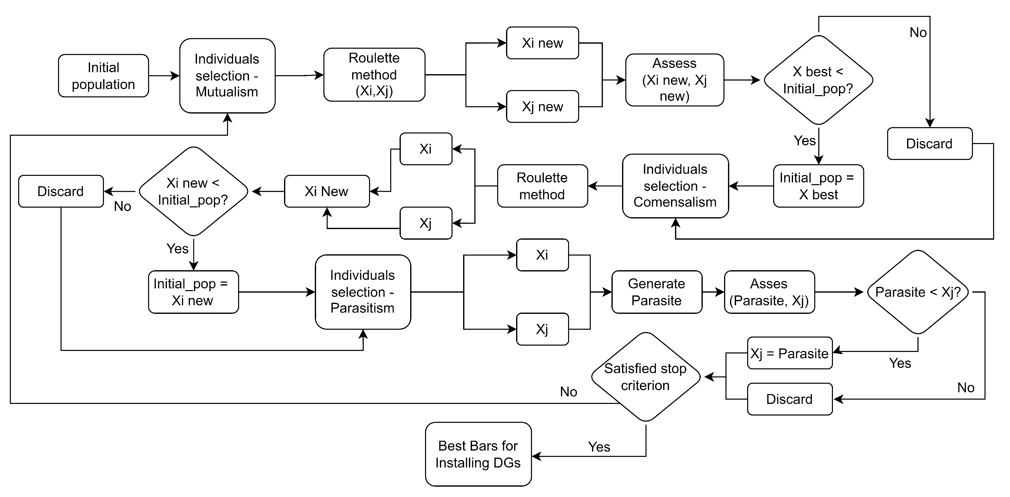
3.2. Symbiotic Organism Search

Living organisms rarely live in isolation, due to their dependence on other organisms for their sustenance for survival. This dependency-based relationship is called symbiosis. The most common symbiotic relationships between two organisms in nature are mutualism, commensalism, and parasitism. In mutualism both organisms benefit, in commensalism one organism is benefited and the other one is not affected, and in parasitism one of the organisms benefits, and the other one is actually harmed.

The symbiotic organism search (SOS) metaheuristic simulates symbiotic relationships with paired organisms, which are used to search for the fittest organism to solve the optimization problem. As in other population-based metaheuristics, the SOS algorithm iteratively uses a population of candidate solutions from promising areas to scan the solution space in search of the global optimum value. Initial organisms are randomly generated in the solution space. Each organism represents a candidate solution to the optimization problem with an associated fitness value, which reflects the degree to which the organism is adapted to the desired objective [50].

In the SOS algorithm, generating a new solution is a process governed by mimicking the biological interactions between two organisms in an ecosystem. Each organism interacts with the others in three phases that resemble the real world: mutualism, commensalism, and parasitism. With each generation, the organisms undergo interactions in each of the symbiotic phases until a predetermined stopping criterion is reached [50].

3.2.1. Mutualistic Phase

An example of mutualism that benefits each participating organism is the relationship between the woodpecker and the buffalo. The woodpecker feeds on insects present on the buffalo’s body, while the buffalo benefits by removing these parasites. In SOS, $X_i$ is the organism occupying the i-th position in the ecosystem. Another organism, $X_j$ is randomly chosen from the population to interact with $X_i$. New solution candidates $X_{inew}$ and $X_{jnew}$ are calculated based on the mutualistic relationship which is modeled as indicated in Equations (13)–(15).

$$X_{inew}=X_i+rand(0,1)\times (X_{best}-\mathrm{Mutual}\_\mathrm{Vector}\times B{F}_1)$$

(13)

$$X_{jnew}=X_j+rand(0,1)\times (X_{best}-\mathrm{Mutual}\_\mathrm{Vector}\times B{F}_2)$$

(14)

$$\mathrm{Mutual}\_\mathrm{Vector}=\frac{X_i+X_j}{2}$$

(15)

In Equations (13) and (14), the term $rand(0,1)$ is a random number between 0 and 1, while $B{F}_1$ and $B{F}_2$ represent how much the organisms will benefit from the mutual relationship. In this case, $B{F}_1$ and $B{F}_2$ vary randomly between 1 and 2.

The mutual vector indicated in Equation (15) represents the mutualism relationship between organisms $X_i$ and $X_j$. The expression $(X_{best}-\mathrm{Mutual}\_\mathrm{Vector}\times BF)$ reflects the mutual effort to achieve a good outcome and ensure survival. The term $X_{best}$ represents the highest degree of fitness in the ecosystem, so using it can help increase the degree of fitness of each of the organisms. Initially, the organisms are updated only if their new fitness values are better than those prior to the organisms’ interaction.

3.2.2. Commensalism Phase

An example of commensalism is the relationship between the shark and the remora. The remora attaches itself to the shark and feeds on the leftover food that the shark leaves behind, while the shark is not affected by the presence and activities of the remora. In this phase, an organism denoted as $X_j$ is randomly chosen to relate to organism $X_i$. Thus, organism $X_i$ benefits from this interaction, while organism $X_j$ suffers no change. A new candidate $X_{inew}$ is calculated in this interaction which is mathematically modeled by Equation (16). Then, organism $X_i$ is updated only if the new organism is fitter than the previous one.

$$X_{inew}=X_i+rand(-1,1)\ast (X_{best}-X_j)$$

(16)

In Equation (16), the term $rand(-1,1)$ represents a random number between −1 and 1, while the expression $(X_{best}-X_j)$ reflects the benefit that organism $X_i$ is receiving from organism $X_j$, increasing its survival advantages in an ecosystem together with the current fittest organism $X_{best}$.

3.2.3. Parasitism Phase

An example of parasitism is the relationship between the chopper and other host birds. The chopper lays its eggs in the nest of another bird, which benefits the chopper because it transfers the job of caring for the chicks to the bird that had its nest invaded, and harms the host because the resources of its offspring will be consumed by the parasite, which can even kill the offspring of the host.

In the parasitism step, organism $X_i$ takes over the role of a parasite by creating an artificial organism called “Parasite Vector”. The parasite vector is created by duplicating vector $X_i$ and randomly changing one of its dimensions. An organism $X_j$ is randomly chosen and serves as a host for the parasite vector. The latter tries to replace $X_j$ organism, so both organisms are evaluated, and if the parasite vector is fitter, it will eliminate $X_j$ organism and assume its position in the ecosystem. The SOS metaheuristic was implemented according to the algorithm described below.

Step 1: Generate an ecosystem of size M, with N-dimensional organisms.

Step 2: Evaluate the fitness of each of the organisms in the ecosystem through IPF, where the fitness function $fi{t}_i$ of each of the organisms is the value of the interval technical losses obtained by IPF. Penalties are applied if a violation in voltage levels is observed. The penalty consists of adding a high value to the objective function that is wanted to minimize. Voltage level violations can be analyzed using Equation (17), where $\dot{V_k^i}$ indicates the range of acceptable voltage values per unit. After that, the fittest organism, $X_{best}$ is identified.

$$\dot{V_k^i}\subset [0.95;1.05]$$

(17)

All organisms in the ecosystem will undergo all the interactions described in phases 1, 2, and 3 at each iteration. The organism undergoing the interaction will be called $X_i$.

Phase 1—Mutualism:

Step 3: Select an organism $X_j$ where $j\ne i$.

Step 4: The mutual vector is calculated by means of Equation (15).

Step 5: New organisms coming from mutualism are calculated using Equations (13) and (14), with the parameters $BF1$ and $BF2$ randomly drawn between 1 and 2.

Step 6: The new organisms are evaluated and if they are fitter than the original organisms, they replace them; otherwise, they are discarded.

Phase 2—Commensalism

Step 7: An organism $X_j$ is selected where $j\ne i$.

Step 8: A new organism is generated through commensalism according to Equation (16).

Step 9: The new organism is evaluated and if it is fitter than the original $X_i$ organism, it replaces it; otherwise, it is discarded.

Phase 3—Parasitism

Step 10: An organism $X_j$ is selected where $j\ne i$.

Step 11: A parasite vector is created by randomly changing one dimension of organism $X_i$.

Step 12: The new parasite organism is evaluated and if it is fitter than organism $X_j$ it replaces it; otherwise, it is discarded.

Step 13: It is checked if i is the last position in the population (if the whole population has passed through the three symbiotic stages), if yes, go to the next step, if no, $i=i+1$ and return to Step 2.

Step 14: It is checked if the stopping criterion has been reached, if not, return to Step 2. If yes, the search for the optimal solution is complete.

Figure 1 presents the flowchart of the implemented SOS algorithm.

3.3. Particle Swarm Optimization

PSO is a metaheuristic technique proposed in [63] and is based on the representation of the movement of organisms in a bird flock or fish school. PSO has shown to be effective for solving several electrical engineering problems such as optimal sitting and sizing of DG [55,56], ancillary service optimization [64], optimal sizing of photovoltaic systems [65], and optimal protection coordination [66], among many others. PSO has also been hybridized to improve its performance, as reported in [67,68,69]. According to the literature, the motion of birds in a flock or schools of fish, which are commonly named swarms, can be based on five principles [63]:

• The proximity principle, where individuals in the population must be able to move around in a search space.
• The quality principle, in which individuals must be able to respond to quality factors in the environment.
• The principle of diverse responses, in which individuals should not be bound to a restricted path.
• The stability principle, in which individuals should not change their behavior whenever environmental conditions change.
• The adaptability principle, in which individuals must be able to change their behavior when it is no longer convenient.

The PSO algorithm starts from the basis of a swarm that is artificially generated in the search space of solutions. Each element of this swarm is called a particle and behaves as a point without mass and volume in an N-dimensional space. Each particle is a candidate solution to the optimization problem. The iterations of these particles are governed by the five principles mentioned above.

PSO is a search algorithm for optimal solutions based on the behavior of a swarm, in which each particle can memorize its own “optimal” value, the “optimal” value of all other particles in the swarm, and its own velocity, and has a fitness value that shows how close that particle is to the optimal position. Thus, in each generation, the particles’ information is combined to generate new velocities for each of the dimensions, which are used to generate a new particle [70]. The flowchart of the implemented PSO is presented in Figure 2.

To describe the PSO algorithm, a swarm of size M in an N-dimensional space is assumed, where the position of each particle i is $X_i=(x_{i1},x_{i2},\dots ,x_{id},.\dots ,x_{iN})$, its velocity is $V_i=(v_{i1},v_{i2},\dots ,v_{id},\dots ,v_{iN})$, and the optimal position that each particle has assumed, that is, the position at which that particle has assumed the best fitness value. This position is given by $P_i=(p_{i1},p_{i2},\dots ,p_{id},\dots ,p_{iN})$. The optimal swarm position, which corresponds to the best of the optimal positions of the particles, is given by $P_g=(p_{gi1},p_{gi2},\dots ,p_{gid},\dots ,p_{giN})$.

Thus, new velocities and positions for the particles can be calculated as:

$$v_{i,t+1}^d=\omega \times v_{i,t}^d+c_1\times rand(0,1)\times (p_{i,t}^d-x_{i,t}^d)+c_2\times rand(0,1)\times (p_{g,t}-x_{i,t}^d)$$

(18)

$$x_{i,t+1}^d=x_{i,t}^d+v_{i,t+1}^d$$

(19)

From Equation (18) it can be seen that the first term $\omega \ast v_{i,t}^d$ represents the influence of the particle’s prior velocity, so parameter $\omega$ is called the inertial weight. The second term, $c_1\times rand(0,1)\times (p_{i,t}^d-x_{i,t}^d)$, represents the distance between the particle and its own optimal position. In this case, parameter $c_1$ is called the cognitive learning factor. The third term, $c_2\times rand(0,1)\times (p_{g,t}-x_{i,t}^d)$, represents the distance between the particle and the optimal swarm position. It represents the fact that particles can share information and cooperate, moving according to the experience of the whole swarm. In this term, the parameter $c_2$ is called the social learning factor.

The velocities and positions of each of the particles are iteratively updated. The local and global maxima, $P_g$ and $P_i$, are recalculated at each iteration until a predetermined stopping criterion is reached.

The PSO metaheuristic was implemented according to the algorithm described below.

Step 1: Generate a swarm of size M, with N-dimensional particles and set iteration zero with variable $iter=0$.

Step 2: Evaluate each particle in the swarm via IPF, where the fitness function $fi{t}_i$ of each of the organisms is the value of interval technical losses obtained by IPF and penalties are applied if a violation in voltage levels is observed. Violations in voltage levels can be analyzed using Equation (17). After that, define the particle with the best position towards the solution $P^g$ in the swarm and also the best position of each of the particles $P^i$.

Step 3: A new velocity for the particles is calculated using Equation (18). In this case, learning factors c1 = 2 and c2 = 1.49445, which are commonly used, are adopted [70]. Furthermore, an inertia factor $\omega$ is used given by Equation (20).

$$\omega ={\omega }_{max}-\frac{{\omega }_{max}-{\omega }_{min}}{max\_iter}\times iter$$

(20)

In Equation (20), $max\_iter$ is the maximum number of iterations, $iter$ is the value of the current iteration, and ${\omega }_{max}$ = 0.9 and ${\omega }_{min}$ = 0.4 are adopted as the maximum and minimum values for the inertial weight, respectively.

Step 4: Check if the stopping criterion $iter=max\_iter$ has been reached, if not, $iter=iter+1$ and return to Step 2, if yes, the optimal solution has been found.

3.4. Metrics

From the information returned by the IPF intervals, it is necessary to define a criterion to evaluate which is the best value of the objective function; that is, the smallest value of the system power losses. In this work, the following comparison methodologies were implemented:

3.4.1. Comparison of the Midpoints

In this method, the interval $X=[x_1,x_2]$ is considered to be smaller than the interval $Y=[y_1,y_2]$ if their midpoints, obtained from Equation (1), follow the following constraint given by Equation (21).

$$X<Y\iff Mid\left(X\right)<Mid\left(Y\right)$$

(21)

3.4.2. Evaluation Using the Interval Measurement Function

In this method, the interval $X=[x_1,x_2]$ is considered to be smaller than the interval $Y=[y_1,y_2]$ if the interval measure function given by Equation (22) returns a value greater than zero, according to Equations (23)–(26) [71], where $m_x$ and $m_y$ represent the midpoint of the intervals X and Y, respectively, while $r_x$ and $r_y$ represent the radius of the intervals, respectively.

$$\mu (X,Y)=\left\{\begin{array}{c}{m}_y-m_x+2·sgn(m_y-m_x),\mathrm{if}{r}_y+r_x=0\hfill \\ \frac{m_y-m_x}{r_y+r_x}+sgn(m_y-m_x),\mathrm{if}{m}_x\ne m_y\mathrm{and}{r}_y+r_x\ne 0\hfill \\ \frac{r_y-r_x}{max\{r_y,r_x\}},\mathrm{if}{m}_x=m_y\mathrm{and}{r}_y+r_x\ne 0\hfill \end{array}\right.$$

(22)

$$m_x=Mid\left(X\right)$$

(23)

$$r_x=Radius\left(X\right)$$

(24)

$$m_y=Mid\left(Y\right)$$

(25)

$$r_y=Radius\left(Y\right)$$

(26)

In this case, $sgn$ is given by Equation (27).

$$sgn\left(x\right)=\left\{\begin{array}{c}-1\mathrm{if}\mathrm{x}<0\hfill \\ 0\mathrm{if}\mathrm{x}=0\hfill \\ 1\mathrm{if}\mathrm{x}>0\hfill \end{array}\right.$$

(27)

Thus, X < Y can be mathematically described by Equation (28).

$$X<Y\iff \mu (X,Y)>0$$

(28)

4. Tests and Results

In this paper, the IPF approach described and validated in [57] was implemented. For the validation of the IPF, a deterministic power flow using the Newton–Rapshon method with sparse matrix treatment was developed. After running the deterministic power flow, the IPF is also processed as described in Section 2 (please see reference [57] for more details). Medium voltage distribution systems with radial topologies were simulated with load variations of $5^{-4}$ between iterations. All tests were carried out considering a single-phase equivalent of the distribution test systems. The stopping criterion considers a maximum variation in the radius of the variables of ${10}^{-4}$ between iterations. All computational simulations were implemented in Python^®.

After the validation of the IPF results, the optimal allocation and sizing of DG in the test networks were developed in Python^® based on the described metaheuristics: SOS [50] and PSO [63]. The DG units allocated by these algorithms were also simulated with 5% variations in their power. Regarding generation technologies, for the sake of simplicity, the proposed approach does not model the intrinsic generation variability of renewable energy resources; instead, an expected generation value is considered for the buses selected for DG allocation. The maximum numbers of iterations were 100 and 250 for the IEEE 33-bus and IEEE 69-bus test systems, respectively.

4.1. Results with the IEEE 33-Bus Test System

4.1.1. System Data

The data on the IEEE 33-bus test system can be found in [72]. This system has a total active load of 3715 kW and a total reactive load of 2300 kvar. The base values considered are 100 kVA and 12.66 kV. The maximum and minimum values of the voltage magnitude, obtained from the deterministic power flow, are 1.0 p.u and 0.909 p.u, respectively.

The optimal allocation and sizing of DG performed on the IEEE 33-bus test systems was carried out considering buses 7, 10, 13, 26, 31, and 33 as eligible for DG allocation. This consideration is based on the fact that in real distribution systems, not all network buses are eligible for DG allocation due to constraints related to the availability of resources as well as land use limitations. It was also considered the restriction that the maximum penetration rate of DG in this system is 30%, that is, the total generation cannot exceed 30% of the grid active load. Thus, for this system, the maximum generation to be allocated is 1114.5 kW.

4.1.2. SOS Applied to the IEEE 33-Bus Test System

The SOS algorithm was processed for the DG allocation, with 100 iterations in an ecosystem of 20 organisms, and had its active power losses evaluated under the two metrics presented in Section 3.4. The amounts of power allocated to each of the buses are presented in

Table 2. Active power of DG allocated per bus by the SOS algorithm in the IEEE 33-bus test network.

Active Power of DG Allocated (kW)
Bus	7	10	13	26	31	33	Total
Midpoint Comparison	0	0	528.2	0	304.8	281.3	1114.4
Evaluation with Interval Measurement Function	0	145.6	410.47	0	527.3	30.63	1114.3

. To validate the results of the SOS algorithm, a convergence analysis was performed using the results of 10 optimization simulations using the midpoint comparison metric.

Table 3. Convergence analysis of the SOS algorithm on the IEEE 33-bus test network.

SOS
Simulation	Lower Limit of Losses (kW)	Upper Limit of Losses (kW)
1	72.95	77.88
2	72.91	77.84
3	71.15	76.88
4	73.20	77.73
5	72.96	77.69
6	73.08	78.01
7	72.83	77.86
8	74.00	78.83
9	72.93	77.76
10	72.91	77.93

presents the results of these simulations. Note that all of them led to similar values, evidencing the convergence of the algorithm.

The proposed methodology only considers the results that meet voltage limits. Figure 3 allows us to verify this criterion. In this case, variables $Vinf\_m1$ and $Vsup\_m1$ are, respectively, the lower and upper bounds of the magnitude of the interval voltages on each of the buses in the solution obtained by the SOS algorithm using the midpoint comparison metric. On the other hand, $Vinf\_m2$ and $Vsup\_m2$ are, respectively, the lower and upper bounds of the magnitude of the interval voltage on each of the buses in the solution obtained by the SOS algorithm, using the evaluation metric via the interval measure function. Finally, $Vinf$ and $Vsup$ are, respectively, the lower and upper bounds of the magnitude of the interval voltage at each of the buses obtained by IPF without DG. Note that there is an important improvement in the voltage profile when DG is included in the network.

Table 4. Interval losses obtained by the SOS algorithm for the IEEE 33-bus network.

Metric	Lower Limit of Losses (kW)	Upper Limit of Losses (kW)
Midpoint comparison	72.95	77.88
Evaluation with Interval Measurement Function	73.14	77.91

presents the values of interval losses obtained by the SOS algorithm for the two metrics used. Figure 4 and Figure 5 show the convergence of the midpoints of the interval losses and their diameters for the two metrics. From Figure 4, it is observed that the convergence of the algorithm is obtained around iteration 55, which shows that the search process aiming at minimum losses is adequate. On the other hand, when the radius of the loss range of the best solution obtained at each iteration is evaluated, it is observed from Figure 5 that the diameter increases over the course of the simulation, i.e., for both metrics the uncertainty of the result increases over the course of the simulation. Also note that the simulation performed by the comparison metric using the interval measure function results in a smaller diameter.

Therefore, according to the results observed, it can be concluded that the SOS algorithm is robust and efficient in solving the DG allocation and sizing problem when both metrics are considered.

4.1.3. PSO Applied to the IEEE 33-Bus Test System

The PSO algorithm considers 100 iterations under a swarm of 20 particles. The active power losses were evaluated, during the process, by means of the two metrics presented in Section 3.4. The amount of power allocated to each bus is indicated in

Table 5. Active power of DG allocated per bus by the PSO algorithm in the IEEE 33-bus test network.

Active Power of DG Allocated (kW)
Bus	7	10	13	26	31	33	Total
Midpoint Comparison	169.6	186.4	172.9	184.1	203.0	191.6	1107.8
Evaluation with Interval Measurement Function	159.1	185.5	169.2	183.0	198.6	214.7	1110.3

.

To validate the results of the PSO algorithm, a convergence analysis was performed using the results of 10 optimization simulations using the midpoint comparison metric.

Table 6. Convergence analysis of the PSO algorithm on the IEEE 33-bus network.

PSO
Simulation	Lower Limit of Losses (kW)	Upper Limit of Losses (kW)
1	82.72	87.10
2	82.52	87.42
3	81.74	87.16
4	82.92	88.54
5	82.59	87.11
6	83.08	87.79
7	82.51	88.22
8	81.61	87.52
9	84.62	89.34
10	82.77	88.58

presents the results of these simulations. Note that all of the values are similar, evidencing the convergence of the algorithm.

According to Equation (17), the methodology only considers the results that satisfy the pre-established voltage limits. Figure 6 evidences the enforcement of this criterion.

In Figure 6, the variables $Vinf\_m1$ and $Vsup\_m1$ are, respectively, the lower and upper bounds of the magnitude of the interval voltage at each bus of the system in the solution obtained by the PSO algorithm using the midpoint comparison metric. The variables $Vinf\_m2$ and $Vsup\_m2$ are, respectively, the lower and upper bounds of the magnitude of the interval voltage at each bus of the system in the solution obtained by the PSO algorithm using the evaluation metric via the interval measure function. Finally, the lines corresponding to $Vinf$ and $Vsup$ are, respectively, the lower and upper bounds of the magnitude of the interval voltage at each bus obtained by the IPF without DG.

Table 7. Interval losses obtained by the PSO algorithm for the IEEE 33-bus network.

Metric	Lower Limit of Losses (kW)	Upper Limit of Losses (kW)
Midpoint Comparison	82.72	87.10
Evaluation with Interval Measurement Function	82.25	86.65

presents the values of interval losses obtained by the PSO algorithm for the two metrics used. Figure 7 and Figure 8 show the convergence of the midpoints of the interval losses and their diameters for the two metrics.

From Figure 7, it is observed that the convergence of the algorithm is obtained around iteration 9. This shows that the search process aiming at minimizing power losses is successful since the midpoint decreases with each iteration. However, it is observed that for both metrics the algorithm is stuck at a local minimum. On the other hand, when evaluating the radius of the loss range of the best solution obtained at each iteration, it is observed in Figure 8 that the radius increases over the course of the simulation, that is, for both metrics, the uncertainty of the result increases over the course of the simulation.

Therefore, regarding the convergence of the PSO algorithm, it can be concluded that it worked correctly when seeking to solve the DG allocation and sizing problem when considering the two metrics, but was not able to escape from local optimal solutions.

4.1.4. Power Loss Comparison

Figure 9 illustrates the values of losses considering midpoint comparison and evaluation with interval measurement function for both PSO and SOS algorithms. It is observed that SOS presents better performance than PSO, where the SOS midpoint is 75.42 MW while the PSO midpoint is 84.92 MW, approximately.

In summary, from the results presented in Section 4.1.2, Section 4.1.3 and Section 4.1.4 it is clear that the SOS algorithm performed better when compared to the PSO. From Figure 7 it is evident that the PSO algorithm was stuck at a local minimum for both metrics.

4.2. Results with the IEEE 69-Bus Test system

4.2.1. System Data

The data for this system can be found in [73]. The base values considered are 100 kVA and 12.66 kV. The 69-bus system has a total active load of 3802.19 kW and a total reactive load of 2694.60 kvar. The maximum and minimum values of the voltage magnitude, obtained from a deterministic power flow, are 1.0 p.u and 0.909 p.u, respectively.

The proposed methodology for optimal allocation and sizing of DG considers the following candidate buses: 10, 18, 27, 40, 49, 54, 62, and 68. It is also considered that the maximum DG penetration rate is 20%, which corresponds to 760.44 kW.

4.2.2. SOS Applied to the IEEE 69-Bus Test System

The SOS algorithm was simulated considering 250 iterations in an ecosystem of 20 organisms. The active power losses are evaluated under the two metrics presented in Section 3.4. The amounts of power allocated as a result of the implemented algorithm at each bus are presented in

Table 8. Active power of DG allocated per bus by the SOS algorithm in the IEEE 69-bus network.

Allocated Distributed Generation Active Power (kW)
Bus	10	18	27	40	49	54	63	68	Total
Midpoint Comparison	0	0	18.72	0	21.32	0	720.4	0	760.44
Evaluation with Interval Measurement Function	13.2	11.1	0	2.91	62.63	0	670.6	0	760.44

.

According to Equation (17), the methodology only considers the results that meet the pre-established voltage limits. Figure 10 allows us to verify this condition.

In Figure 10, the lines corresponding to $Vinf\_m1$ and $Vsup\_m1$ are, respectively, the lower and upper bounds of the magnitude of the interval voltage on the system buses in the solution obtained by the SOS algorithm, using the midpoint comparison metric. The lines of variables $Vinf\_m2$ and $Vsup\_m2$ are, respectively, the lower and upper bounds of the magnitude of the interval voltage on the system buses in the solution obtained by the SOS algorithm, using the evaluation metric via the interval measure function. $Vinf$ and $Vsup$ indicate, respectively, the lower and upper bounds of the magnitude of the interval voltage obtained by the IPF without DG.

The interval losses obtained by the SOS algorithm are presented in

Table 9. Interval losses obtained by the SOS algorithm for the IEEE 69-bus test network.

Metric	Lower Limit of Losses (kW)	Upper Limit of Losses (kW)
Midpoint Comparison	79.7	129.5
Evaluation Using the Interval Measurement Function	85.7	135.3

. Figure 11 and Figure 12 show the convergence of the midpoints of the interval losses and their diameters for the two metrics. From Figure 11, it can be inferred that the convergence of the algorithm is obtained around iteration 92. On the other hand, when the diameter of the loss range of the best solution obtained at each iteration is evaluated, it can be seen in Figure 12 that the radius varies during the simulation. Also note that simulation performed by the comparison metric using the interval measure function results in a smaller diameter.

Therefore, regarding the convergence of the SOS algorithm, it was observed that the algorithm is robust and efficient in solving the DG allocation and sizing problem when both metrics are considered.

4.2.3. PSO Applied to the IEEE 69-Bus Test System

The PSO algorithm was run considering 250 iterations on a swarm of 20 particles. The active power losses are evaluated under the two metrics presented in Section 3.4. The amounts of power allocated to the candidate buses are presented in

Table 10. Active power of DG allocated per bar by the SOS algorithm in the IEEE 69-bus network.

Allocated Distributed Generation Active Power (kW)
Bus	10	18	27	40	49	54	63	68	Total
Midpoint Comparison	69.9	118.1	95.47	52.9	86	102.8	115.1	88.5	728.7
Evaluation with Interval Measurement Function	92.9	97.5	82.3	100.5	75.7	97.3	114.1	85.3	745.7

.

As already mentioned, the proposed approach only considers results that meet voltage limits. This can be verified in Figure 13, where $Vinf\_m1$ and $Vsup\_m1$ are the lower and upper bounds of the magnitude of the interval voltage on the system buses in the solution obtained by the PSO algorithm, using the midpoint comparison metric. The lines of variables $Vinf\_m2$ and $Vsup\_m2$ are, respectively, the lower and upper bounds of the magnitude of the interval voltage on the system buses in the solution obtained by the PSO algorithm, using the evaluation metric via the interval measure function. Finally, the variables $Vinf$ and $Vsup$ are, respectively, the lower and upper bounds of the magnitude of the interval voltage on the system buses obtained by IPF without DG.

Table 11. Interval losses obtained by the PSO algorithm for the IEEE 69-bus network.

Metric	Lower Limit of Losses (kW)	Upper Limit of Losses (kW)
Midpoint Comparison	145.56	193.70
Evaluation with Interval Measurement Function	148.77	196.30

shows the interval loss values obtained by the PSO algorithm for the two metrics used. Figure 14 and Figure 15 show the convergence of the midpoints of the interval losses and their diameters for the two metrics. From Figure 14, it is observed that the convergence of the algorithm is obtained around iteration 9 and, it shows that the search process aiming at minimum losses is adequate since the midpoint decreases with each iteration. However, it is clearly observed that for both metrics the algorithm is stuck in a local minimum. On the other hand, when evaluating the radius of the loss range of the best solution obtained at each iteration, it is observed from Figure 15 that the diameter increases over the course of the simulation, i.e., for both metrics the uncertainty of the result increases over the course of the simulation. Also note that the simulation performed by the comparison metric using the interval measure function results in a smaller diameter.

Therefore, regarding the convergence of the PSO algorithm, it was observed that the algorithm worked correctly in trying to solve the DG allocation and sizing when considering the two metrics, but it was not able to escape from local optimal solutions. Furthermore, the solution at which the algorithm was stuck is not even able to regulate the feeder voltage within the desired limits.

4.2.4. Power Loss Comparison

Figure 16 presents the power losses considering midpoint comparison and evaluation with interval measurement function for the metaheuristics under study. Note that the midpoint of lower power losses obtained with the SOS and PSO approaches approximately correspond to 104.57 MW and 169.63 MW, respectively.

In summary, from the results presented in Section 4.2.2, Section 4.2.3 and Section 4.2.4 it is observed that the SOS algorithm performed better when compared to the PSO. Additionally, according to Figure 14, it is evident that the PSO algorithm was stuck at a local minimum for both metrics.

5. Conclusions

This paper presented an optimal location and sizing approach of DG in distribution networks using PSO and SOS metaheuristics; furthermore, the proposed approach implements an interval power flow that adds uncertainty to the optimization problem. The results obtained in the two distribution test systems evidenced the superiority of the SOS methodology over PSO. With the parameters and modeling used in this work, the SOS metaheuristic obtained better results in all simulations. One of the advantages of SOS over PSO lies in the fact that SOS does not require configuration or fine-tuning of parameters. The implemented methodologies were evaluated using two different metrics, the midpoint comparison and the interval evaluation function. From the results obtained, both metrics present equivalent results; however, the interval evaluation function results show a smaller diameter.

In particular, for the IEEE 69-bus network, it was observed that the PSO algorithm did not perform well, not even being able to propose a solution capable of meeting the constraints regarding the system voltage levels. Nonetheless, in cases where the optimal solutions involved the allocation of DG in all candidate buses, the PSO algorithm showed reasonable results. The PSO algorithm did not have good convergence when considering the simultaneity of the DG allocation and sizing problems; however, according to the results obtained, adequate convergence can be expected when only the sizing problem is addressed.

The SOS algorithm using IPF showed to be a robust methodology capable of adding uncertainty to the optimal location and sizing problem of DG units in distribution systems, which is becoming increasingly common in modern power distribution systems.

References

1. Bai, X.; Qu, L.; Qiao, W. Robust AC Optimal Power Flow for Power Networks With Wind Power Generation. IEEE Trans. Power Syst. 2016, 31, 4163–4164. [Google Scholar] [CrossRef]
2. Lopez-lezama, J.M.; Murillo-Sanchez, C.; Zuluaga, L.; Gutierrez-Gomez, J. A Contingency-Based Security-Constrained Optimal Power Flow Model for Revealing the Marginal Cost of a Blackout Risk-Equalizing Policy in the Colombian Electricity Market. In Proceedings of the 2006 IEEE/PES Transmission Distribution Conference and Exposition: Latin America, Caracas, Venezuela, 15–18 August 2006; pp. 1–6. [Google Scholar] [CrossRef]
3. Bian, J.; Wang, H.; Wang, L.; Li, G.; Wang, Z. Probabilistic optimal power flow of an AC/DC system with a multiport current flow controller. CSEE J. Power Energy Syst. 2021, 7, 744–752. [Google Scholar] [CrossRef]
4. Amiri, H.; Mohammadi, M.; Karimi, M.; Rastegar, M.; Rostami, A. Probabilistic Load Flow Based on Parameterized Probability-Boxes for Systems with Insufficient Information. IEEE Access 2021, 9, 161038–161045. [Google Scholar] [CrossRef]
5. Villada Duque, F.; López Lezama, J.M.; Muñoz Galeano, N. Effects of Incentives for Renewable Energy in Colombia. Ing. Univ. 2017, 21, 257–272. [Google Scholar] [CrossRef] [Green Version]
6. Strezoski, L.; Padullaparti, H.; Ding, F.; Baggu, M. Integration of Utility Distributed Energy Resource Management System and Aggregators for Evolving Distribution System Operators. J. Mod. Power Syst. Clean Energy 2022, 10, 277–285. [Google Scholar] [CrossRef]
7. Ryu, J.; Kim, J. Virtual Power Plant Operation Strategy Under Uncertainty with Demand Response Resources in Electricity Markets. IEEE Access 2022, 10, 62763–62771. [Google Scholar] [CrossRef]
8. Rezaei, E.; Dagdougui, H.; Ojand, K. Hierarchical Distributed Energy Management Framework for Multiple Greenhouses Considering Demand Response. IEEE Trans. Sustain. Energy 2023, 14, 453–464. [Google Scholar] [CrossRef]
9. Primadianto, A.; Lu, C. A Review on Distribution System State Estimation. IEEE Trans. Power Syst. 2017, 32, 3875–3883. [Google Scholar] [CrossRef]
10. de Oliveira, L.W.; Seta, F.d.S.; de Oliveira, E.J. Optimal reconfiguration of distribution systems with representation of uncertainties through interval analysis. Int. J. Electr. Power Energy Syst. 2016, 83, 382–391. [Google Scholar] [CrossRef]
11. Pereira, L.; da Costa, V.; Rosa, A. Interval arithmetic in current injection power flow analysis. Int. J. Electr. Power Energy Syst. 2012, 43, 1106–1113. [Google Scholar] [CrossRef]
12. Araujo, B.M.C.; da Costa, V.M. New Developments in the Interval Current Injection Power Flow Formulation. IEEE Lat. Am. Trans. 2018, 16, 1969–1976. [Google Scholar] [CrossRef]
13. Seta, F.D.S.; de Oliveira, L.W.; de Oliveira, E.J. Distribution System Planning with Representation of Uncertainties Based on Interval Analysis. J. Control Autom. Electr. Syst. 2020, 31, 494–510. [Google Scholar] [CrossRef]
14. Mori, H.; Yuihara, A. Calculation of multiple power flow solutions with the Krawczyk method. In Proceedings of the 1999 IEEE International Symposium on Circuits and Systems (ISCAS), Orlando, FL, USA, 30 May–2 June 1999; Volume 5, pp. 94–97. [Google Scholar] [CrossRef]
15. Rasmussen, T.B.; Yang, G.; Nielsen, A.H. Interval estimation of voltage magnitude in radial distribution feeder with minimal data acquisition requirements. Int. J. Electr. Power Energy Syst. 2019, 113, 281–287. [Google Scholar] [CrossRef]
16. Lin, X.; Shu, T.; Tang, J.; Ponci, F.; Monti, A.; Li, W. Application of Joint Raw Moments-Based Probabilistic Power Flow Analysis for Hybrid Power Systems. IEEE Trans. Power Syst. 2022, 37, 1399–1412. [Google Scholar] [CrossRef]
17. Li, Y.; Wan, C.; Chen, D.; Song, Y. Nonparametric Probabilistic Optimal Power Flow. IEEE Trans. Power Syst. 2022, 37, 2758–2770. [Google Scholar] [CrossRef]
18. Shu, T.; Lin, X.; Peng, S.; Du, X.; Chen, H.; Li, F.; Tang, J.; Li, W. Probabilistic Power Flow Analysis for Hybrid HVAC and LCC-VSC HVDC System. IEEE Access 2019, 7, 142038–142052. [Google Scholar] [CrossRef]
19. Peng, S.; Lin, X.; Tang, J.; Xie, K.; Ponci, F.; Monti, A.; Li, W. Probabilistic Power Flow of AC and DC Hybrid Grids With Addressing Boundary Issue of Correlated Uncertainty Sources. IEEE Trans. Sustain. Energy 2022, 13, 1607–1619. [Google Scholar] [CrossRef]
20. Fu, C.; Xu, Y.; Yang, Y.; Lu, K.; Gu, F.; Ball, A. Response analysis of an accelerating unbalanced rotating system with both random and interval variables. J. Sound Vib. 2020, 466, 115047. [Google Scholar] [CrossRef]
21. Cheng, W.; Cheng, R.; Shi, J.; Zhang, C.; Sun, G.; Hua, D. Interval Power Flow Analysis Considering Interval Output of Wind Farms through Affine Arithmetic and Optimizing-Scenarios Method. Energies 2018, 11, 3176. [Google Scholar] [CrossRef] [Green Version]
22. Luo, L.; Gu, W.; Wang, Y.; Chen, C. An Affine Arithmetic-Based Power Flow Algorithm Considering the Regional Control of Unscheduled Power Fluctuation. Energies 2017, 10, 1794. [Google Scholar] [CrossRef] [Green Version]
23. Wang, Y.; Wu, Z.; Dou, X.; Hu, M.; Xu, Y. Interval power flow analysis via multi-stage affine arithmetic for unbalanced distribution network. Electr. Power Syst. Res. 2017, 142, 1–8. [Google Scholar] [CrossRef]
24. Wang, C.; Liu, D.; Tang, F.; Liu, C. A clustering-based analytical method for hybrid probabilistic and interval power flow. Int. J. Electr. Power Energy Syst. 2021, 126, 106605. [Google Scholar] [CrossRef]
25. Zhang, C.; Chen, H.; Shi, K.; Qiu, M.; Hua, D.; Ngan, H. An Interval Power Flow Analysis Through Optimizing-Scenarios Method. IEEE Trans. Smart Grid 2018, 9, 5217–5226. [Google Scholar] [CrossRef]
26. Liao, X.; Liu, K.; Zhang, Y.; Wang, K.; Qin, L. Interval method for uncertain power flow analysis based on Taylor inclusion function. Transm. Distrib. IET Gener. 2017, 11, 1270–1278. [Google Scholar] [CrossRef]
27. Liu, B.; Huang, Q.; Zhao, J.; Hu, W. A Computational Attractive Interval Power Flow Approach With Correlated Uncertain Power Injections. IEEE Trans. Power Syst. 2020, 35, 825–828. [Google Scholar] [CrossRef]
28. Zhang, C.; Chen, H.; Ngan, H.; Yang, P.; Hua, D. A Mixed Interval Power Flow Analysis Under Rectangular and Polar Coordinate System. IEEE Trans. Power Syst. 2017, 32, 1422–1429. [Google Scholar] [CrossRef]
29. Tang, K.; Dong, S.; Zhu, C.; Song, Y. Affine Arithmetic-Based Coordinated Interval Power Flow of Integrated Transmission and Distribution Networks. IEEE Trans. Smart Grid 2020, 11, 4116–4132. [Google Scholar] [CrossRef]
30. Çelik, D.; Meral, M.E. Current control based power management strategy for distributed power generation system. Control Eng. Pract. 2019, 82, 72–85. [Google Scholar] [CrossRef]
31. Chen, G.; Lewis, F.L.; Feng, E.N.; Song, Y. Distributed Optimal Active Power Control of Multiple Generation Systems. IEEE Trans. Ind. Electron. 2015, 62, 7079–7090. [Google Scholar] [CrossRef]
32. Machado, L.F.M.; Santo, S.G.D.; Junior, G.M.; Itiki, R.; Manjrekar, M.D. Multi-Source Distributed Energy Resources Management System Based on Pattern Search Optimal Solution Using Nonlinearized Power Flow Constraints. IEEE Access 2021, 9, 30374–30385. [Google Scholar] [CrossRef]
33. Ackermann, T.; Andersson, G.; Söder, L. Distributed generation: A definition. Electr. Power Syst. Res. 2001, 57, 195–204. [Google Scholar] [CrossRef]
34. Saldarriaga-Zuluaga, S.D.; López-Lezama, J.M.; Muñoz-Galeano, N. An Approach for Optimal Coordination of Over-Current Relays in Microgrids with Distributed Generation. Electronics 2020, 9, 1740. [Google Scholar] [CrossRef]
35. Rajagopalan, A.; Swaminathan, D.; Alharbi, M.; Sengan, S.; Montoya, O.D.; El-Shafai, W.; Fouda, M.M.; Aly, M.H. Modernized Planning of Smart Grid Based on Distributed Power Generations and Energy Storage Systems Using Soft Computing Methods. Energies 2022, 15, 8889. [Google Scholar] [CrossRef]
36. Gallego Pareja, L.A.; López-Lezama, J.M.; Gómez Carmona, O. A Mixed-Integer Linear Programming Model for the Simultaneous Optimal Distribution Network Reconfiguration and Optimal Placement of Distributed Generation. Energies 2022, 15, 3063. [Google Scholar] [CrossRef]
37. Pérez Posada, A.F.; Villegas, J.G.; López-Lezama, J.M. A Scatter Search Heuristic for the Optimal Location, Sizing and Contract Pricing of Distributed Generation in Electric Distribution Systems. Energies 2017, 10, 1449. [Google Scholar] [CrossRef] [Green Version]
38. Zhang, C.; Li, J.; Zhang, Y.J.; Xu, Z. Optimal Location Planning of Renewable Distributed Generation Units in Distribution Networks: An Analytical Approach. IEEE Trans. Power Syst. 2018, 33, 2742–2753. [Google Scholar] [CrossRef]
39. Afraz, A.; Malekinezhad, F.; Shenava, S.; Jlili, A. Optimal sizing and sitting in radial standard system using pso. Am. J. Sci. Res. 2012, 67, 50–58. [Google Scholar]
40. Mareddy, P.; Reddy, V.; Vyza, U. Optimal DG placement for minimum real power loss in radial distribution systems using PSO. J. Theor. Appl. Inf. Technol. 2010, 13, 107–116. [Google Scholar]
41. Sedighizadeh, M.; Rezazadeh, A. Using Genetic Algorithm for Distributed Generation Allocation to Reduce Losses and Improve Voltage Profile. Int. J. Comput. Syst. Eng. 2008, 2, 50–55. [Google Scholar]
42. Liu, K.Y.; Sheng, W.; Liu, Y.; Meng, X.; Liu, Y. Optimal sitting and sizing of DGs in distribution system considering time sequence characteristics of loads and DGs. Int. J. Electr. Power Energy Syst. 2015, 69, 430–440. [Google Scholar] [CrossRef]
43. Bhadoria, V.S.; Pal, N.S.; Shrivastava, V.; Jaiswal, S.P. Reliability Improvement of Distribution System by Optimal Sitting and Sizing of Disperse Generation. Int. J. Reliab. Qual. Saf. Eng. 2017, 24, 1740006. [Google Scholar] [CrossRef]
44. Abou El-Ela, A.; Allam, S.; Shatla, M. Maximal optimal benefits of distributed generation using genetic algorithms. Electr. Power Syst. Res. 2010, 80, 869–877. [Google Scholar] [CrossRef]
45. Moradi, M.; Abedini, M. A novel method for optimal DG units capacity and location in Microgrids. Int. J. Electr. Power Energy Syst. 2016, 75, 236–244. [Google Scholar] [CrossRef]
46. Moradi, M.H.; Abedini, M.; Hosseinian, S.M. A Combination of Evolutionary Algorithm and Game Theory for Optimal Location and Operation of DG from DG Owner Standpoints. IEEE Trans. Smart Grid 2016, 7, 608–616. [Google Scholar] [CrossRef]
47. Ameli, A.; Farrokhifard, M.R.; Davari-nejad, E.; Oraee, H.; Haghifam, M.R. Profit-Based DG Planning Considering Environmental and Operational Issues: A Multiobjective Approach. IEEE Syst. J. 2017, 11, 1959–1970. [Google Scholar] [CrossRef]
48. Ali, A.; Keerio, M.U.; Laghari, J.A. Optimal Site and Size of Distributed Generation Allocation in Radial Distribution Network Using Multi-objective Optimization. J. Mod. Power Syst. Clean Energy 2021, 9, 404–415. [Google Scholar] [CrossRef]
49. Purlu, M.; Turkay, B.E. Optimal Allocation of Renewable Distributed Generations Using Heuristic Methods to Minimize Annual Energy Losses and Voltage Deviation Index. IEEE Access 2022, 10, 21455–21474. [Google Scholar] [CrossRef]
50. Cheng, M.Y.; Prayogo, D. Symbiotic Organisms Search: A new metaheuristic optimization algorithm. Comput. Struct. 2014, 139, 98–112. [Google Scholar] [CrossRef]
51. Sanjay, R.; Jayabarathi, T.; Raghunathan, T.; Ramesh, V.; Mithulananthan, N. Optimal Allocation of Distributed Generation Using Hybrid Grey Wolf Optimizer. IEEE Access 2017, 5, 14807–14818. [Google Scholar] [CrossRef]
52. Farh, H.M.H.; Al-Shaalan, A.M.; Eltamaly, A.M.; Al-Shamma’A, A.A. A Novel Crow Search Algorithm Auto-Drive PSO for Optimal Allocation and Sizing of Renewable Distributed Generation. IEEE Access 2020, 8, 27807–27820. [Google Scholar] [CrossRef]
53. Eid, A.; Kamel, S.; Korashy, A.; Khurshaid, T. An Enhanced Artificial Ecosystem-Based Optimization for Optimal Allocation of Multiple Distributed Generations. IEEE Access 2020, 8, 178493–178513. [Google Scholar] [CrossRef]
54. Nayeripour, M.; Mahboubi-Moghaddam, E.; Aghaei, J.; Azizi-Vahed, A. Multi-objective placement and sizing of DGs in distribution networks ensuring transient stability using hybrid evolutionary algorithm. Renew. Sustain. Energy Rev. 2013, 25, 759–767. [Google Scholar] [CrossRef]
55. da Rosa, W.; Gerez, C.; Belati, E. Optimal Distributed Generation Allocating Using Particle Swarm Optimization and Linearized AC Load Flow. IEEE Lat. Am. Trans. 2018, 16, 2665–2670. [Google Scholar] [CrossRef]
56. Arif, S.M.; Hussain, A.; Lie, T.T.; Ahsan, S.M.; Khan, H.A. Analytical Hybrid Particle Swarm Optimization Algorithm for Optimal Siting and Sizing of Distributed Generation in Smart Grid. J. Mod. Power Syst. Clean Energy 2020, 8, 1221–1230. [Google Scholar] [CrossRef]
57. Nogueira, W.C.; Garcés Negrete, L.P.; López-Lezama, J.M. Interval Load Flow for Uncertainty Consideration in Power Systems Analysis. Energies 2021, 14, 642. [Google Scholar] [CrossRef]
58. Alinejad-Beromi, Y.; Sedighizadeh, M.; Sadighi, M. A particle swarm optimization for sitting and sizing of Distributed Generation in distribution network to improve voltage profile and reduce THD and losses. In Proceedings of the 2008 43rd International Universities Power Engineering Conference, Padova, Italy, 1–4 September 2008; pp. 1–5. [Google Scholar] [CrossRef]
59. Saldarriaga-Zuluaga, S.D.; López-Lezama, J.M.; Muñoz-Galeano, N. Adaptive protection coordination scheme in microgrids using directional over-current relays with non-standard characteristics. Heliyon 2021, 7, e06665. [Google Scholar] [CrossRef] [PubMed]
60. Gendreau, M.; Potvin, J.Y. Handbook of Metaheuristics; Springer: New York, NY, USA, 2010; Volume 2. [Google Scholar]
61. Radosavljević, J.; Arsić, N.; Milovanović, M.; Ktena, A. Optimal Placement and Sizing of Renewable Distributed Generation Using Hybrid Metaheuristic Algorithm. J. Mod. Power Syst. Clean Energy 2020, 8, 499–510. [Google Scholar] [CrossRef]
62. Ellahi, M.; Abbas, G. A Hybrid Metaheuristic Approach for the Solution of Renewables-Incorporated Economic Dispatch Problems. IEEE Access 2020, 8, 127608–127621. [Google Scholar] [CrossRef]
63. Kennedy, J.; Eberhart, R. Particle swarm optimization. In Proceedings of the ICNN’95—International Conference on Neural Networks, Perth, WA, Australia, 27 November–1 December 1995; Volume 4, pp. 1942–1948. [Google Scholar] [CrossRef]
64. Dos Santos Alonso, A.M.; Pereira Junior, B.R.; Brandao, D.I.; Marafao, F.P. Optimized Exploitation of Ancillary Services: Compensation of Reactive, Unbalance and Harmonic Currents Based on Particle Swarm Optimization. IEEE Lat. Am. Trans. 2021, 19, 314–325. [Google Scholar] [CrossRef]
65. Silva de Souza, J.; Percy Molina, Y.; Silva de Araujo, C.; Pereira de Farias, W.; Santos de Araujo, I. Modified Particle Swarm Optimization Algorithm for Sizing Photovoltaic System. IEEE Lat. Am. Trans. 2017, 15, 283–289. [Google Scholar] [CrossRef]
66. Ghanbari, M.; Gandomkar, M.; Nikoukar, J. Protection Coordination of Bidirectional Overcurrent Relays Using Developed Particle Swarm Optimization Approach Considering Distribution Generation Penetration and Fault Current Limiter Placement. IEEE Can. J. Electr. Comput. Eng. 2021, 44, 143–155. [Google Scholar] [CrossRef]
67. Prashant; Sarwar, M.; Siddiqui, A.S.; Ghoneim, S.S.M.; Mahmoud, K.; Darwish, M.M.F. Effective Transmission Congestion Management via Optimal DG Capacity Using Hybrid Swarm Optimization for Contemporary Power System Operations. IEEE Access 2022, 10, 71091–71106. [Google Scholar] [CrossRef]
68. Zhen, L.; Liu, Y.; Dongsheng, W.; Wei, Z. Parameter Estimation of Software Reliability Model and Prediction Based on Hybrid Wolf Pack Algorithm and Particle Swarm Optimization. IEEE Access 2020, 8, 29354–29369. [Google Scholar] [CrossRef]
69. Dabhi, D.; Pandya, K. Enhanced Velocity Differential Evolutionary Particle Swarm Optimization for Optimal Scheduling of a Distributed Energy Resources With Uncertain Scenarios. IEEE Access 2020, 8, 27001–27017. [Google Scholar] [CrossRef]
70. Wang, D.; Tan, D.; Liu, L. Particle swarm optimization algorithm: An overview. Soft Comput. 2018, 22, 387–408. [Google Scholar] [CrossRef]
71. Alolyan, I. A new method for comparing closed intervals. Aust. J. Math. Anal. Appl. 2011, 8, 1–6. [Google Scholar]
72. Alam, A.; Gupta, A.; Bindal, P.; Siddiqui, A.; Zaid, M. Power Loss Minimization in a Radial Distribution System with Distributed Generation. In Proceedings of the 2018 International Conference on Power, Energy, Control and Transmission Systems (ICPECTS), Chennai, India, 22–23 February 2018; pp. 21–25. [Google Scholar] [CrossRef]
73. Baran, M.E.; Wu, F.F. Optimal capacitor placement on radial distribution systems. IEEE Trans. Power Deliv. 1989, 4, 725–734. [Google Scholar] [CrossRef]
Figure 1. Flowchart of the implemented SOS algorithm.
Sustainability 15 05171 g001
Figure 2. Flowchart of the implemented PSO.
Sustainability 15 05171 g002
Figure 3. Voltage profile of the IEEE 33-bus test system—SOS.
Sustainability 15 05171 g003
Figure 4. Convergence of SOS algorithm for the IEEE 33-bus test system—midpoints.
Sustainability 15 05171 g004
Figure 5. Convergence of SOS algorithm for the IEEE 33-bus test system—diameters.
Sustainability 15 05171 g005
Figure 6. Voltage profile of the IEEE 33-bus test system—PSO.
Sustainability 15 05171 g006
Figure 7. Convergence of the PSO algorithm for the IEEE 33-bus test system—midpoints.
Sustainability 15 05171 g007
Figure 8. Convergence of the PSO algorithm for the IEEE 33-bus test system—diameters.
Sustainability 15 05171 g008
Figure 9. Convergence of PSO and SOS—33-bus test system.
Sustainability 15 05171 g009
Figure 10. Voltage profile of the IEEE 69-bus test system—SOS.
Sustainability 15 05171 g010
Figure 11. Convergence of the SOS algorithm for the IEEE 69-bus—midpoints.
Sustainability 15 05171 g011
Figure 12. Convergence of the SOS algorithm for the IEEE 69-bus—diameters.
Sustainability 15 05171 g012
Figure 13. Voltage profile of the IEEE 69-bus test system—PSO.
Sustainability 15 05171 g013
Figure 14. Convergence of the PSO algorithm for the IEEE 69-bus test system—midpoints.
Sustainability 15 05171 g014
Figure 15. Convergence of the PSO algorithm for the IEEE 69-bus test system—diameters.
Sustainability 15 05171 g015
Figure 16. Power loss comparison between PSO and SOS—69-bus test system.
Sustainability 15 05171 g016